U.S. Department of Transportation
Federal Highway Administration
1200 New Jersey Avenue, SE
Washington, DC 20590
202-366-4000
Federal Highway Administration Research and Technology
Coordinating, Developing, and Delivering Highway Transportation Innovations
| REPORT |
| This report is an archived publication and may contain dated technical, contact, and link information |
|
| Publication Number: FHWA-HRT-17-013 Date: February 2017 |
Publication Number: FHWA-HRT-17-013 Date: February 2017 |
CFD modeling was conducted to supplement the physical experiments by expanding the range of bridge opening widths and contraction ratios to validate and further develop the conceptual model described in chapter 3. The CFD experiments were used for comparative purposes to evaluate the relative effects of alternative riprap apron designs, particularly partial-width buried installations, to support development of design guidelines. CFD and physical modeling results were not compared. With respect to the conceptual model described in chapter 3, one objective of the CFD modeling was to determine a function for the parameter ε given in the equation in figure 55.
Numerical models were developed with and without riprap aprons to obtain the bed shear stresses tR and tB, respectively. The following four general sets of models were developed and analyzed:
For the flush installations at both the model and prototype scales, the riprap was modeled as recommended in HEC-23 DG 14.(3) The riprap apron extended into the channel at a distance from the abutment of 2y0 (not to exceed 25 ft (7.6 m)) and upstream and downstream at a distance from the abutment of 2y0 (not less than 25 ft (7.6 m)). The channels were trapezoidal with 1:2 (V:H) side slopes, as shown for with and without riprap conditions in figure 78.
An additional set of models were prepared for the buried installation. The same channel geometry and riprap installation were used for these runs except the apron was located so that the top of the riprap layer was located at the contraction scour depth. That is, the apron was buried below the original bed elevation by the estimated contraction depth. The CFD runs were performed assuming this bed material had been eroded away and the riprap apron was exposed. The geometry for these models is shown in figure 79.
The alternative channel shape models differed from one another by the setback of the abutment face to the bottom of the trapezoidal channel, as shown in figure 80. The top geometry was used for the buried installation comparisons. The other two represented a short extension in the setback and a long extension in the setback. The setbacks were 0.98, 2.53, and 3.97 ft (0.30, 0.77, and 1.21 m), respectively.
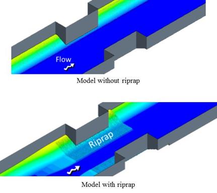 |
| Figure 78. Schematics. Comparison of CFD models for flush installation. |
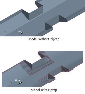 |
| Figure 79. Schematics. Comparison of CFD models for buried installation. |
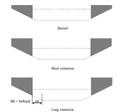 |
| Figure 80. Schematics. Comparison of channel setback alternatives. |
To study the interaction between bed shear stress and riprap for bridge openings of different widths and the effects of flush versus buried installations, a series of bridge opening models with a range of W2 and riprap sizes were built in CFD simulation and are summarized in table 2.
| W2/y0 | Model Scale | Prototype Scale | |||||
|---|---|---|---|---|---|---|---|
| Flush Group #1 |
Flush Group #2 |
Flush Group #3 |
Flush Group #4 |
Flush Group #5 |
Flush Group #6 |
Buried Group #7 |
|
| 6.2 | Case 1 | Case 6 | Case 11 | Case 16 | Case 21 | Case 26 | Case 31 |
| 8 | Case 2 | Case 7 | Case 12 | Case 17 | Case 22 | Case 27 | Case 32 |
| 10 | Case 3 | Case 8 | Case 13 | Case 18 | Case 23 | Case 28 | Case 33 |
| 12 | Case 4 | Case 9 | Case 14 | Case 19 | Case 24 | Case 29 | Case 34 |
| 16 | Case 5 | Case 10 | Case 15 | Case 20 | Case 25 | Case 30 | Case 35 |
| Riprap D50 (inches) |
0.91 | 1.38 | 2.07 | 9.06 | 13.78 | 20.67 | 20.67 |
| 1 inch = 25.4 mm. | |||||||
Each case consisted of two CFD models—one with and one without a riprap apron—so that the ratio of τR /τB could be estimated. A total of 35 cases (70 models) were established and divided into several groups. The first three groups of numerical models were built at a model scale. Case 1 most closely resembled the physical tests performed at the TFHRC and discussed in chapter 4.
The subsequent groups were built in prototype scale with a length ratio of 10 (prototype to model). The prototype tests were conducted to demonstrate that CFD modeling effectively represents both model and prototype scales.
The first six groups used a flush installation of the riprap apron, while the last group used a buried installation. Each group consisted of five cases for bridge openings with W2/y0 ranging from 6.2 to 16. Constants within each group were the riprap size D50 and velocity in the opening V2. The riprap size is determined by the sizing equation in HEC-23 (DG14), as shown in figure 81.(3)
![]()
Figure 81. Equation. HEC-23 (DG14) riprap sizing.
Where:
K = Coefficient (0.89 for a spill-through abutment and 1.02 for vertical-wall abutment) (dimensionless).
An additional series of CFD models were developed and run to investigate the effects of alternative channel setbacks and are summarized in table 3. All of these cases were at prototype scale and only included the natural bed material; no riprap aprons were evaluated.
Table 3. CFD test matrix for alternative setbacks.
| W2/y0 | Short Extension Slope |
Long Extension Slope |
|---|---|---|
| 8 | Case 36 | Case 40 |
| 10 | Case 37 | Case 41 |
| 12 | Case 38 | Case 42 |
| 16 | Case 39 | Case 43 |
Bed shear stress distributions and cross-section velocity distributions of the central cross sections for each of the CFD models were determined. The results are discussed for the flush installation of riprap, the buried installation of riprap, and the alternative channel setback cases.
Table 4 summarizes the defining parameters for each case, including the geometry, riprap size, bed material size, and hydraulics for the flush and buried installation riprap cases. Table 5 summarizes the shear stress and other results from the runs. The equivalent width was the cross-section area divided by the depth.
| Group | Case | Riprap D50 (inches) |
Bed D50 (inches) |
W1 (ft) |
y1 (ft) |
A1 (ft2) |
V1 (ft/s) |
W2 (ft) |
y0 (ft) |
y2 (ft) |
V2 (ft/s) |
|---|---|---|---|---|---|---|---|---|---|---|---|
| Flush Group #1 | 1 | 0.91 | 0.04 | 6.57 | 0.77 | 3.9 | 1.24 | 3.87 | 0.62 | 0.77 | 1.61 |
| 2 | 0.91 | 0.04 | 7.68 | 0.77 | 4.8 | 1.30 | 4.99 | 0.62 | 0.77 | 1.61 | |
| 3 | 0.91 | 0.04 | 8.93 | 0.77 | 5.7 | 1.35 | 6.23 | 0.62 | 0.77 | 1.61 | |
| 4 | 0.91 | 0.04 | 10.18 | 0.77 | 6.7 | 1.39 | 7.48 | 0.62 | 0.77 | 1.61 | |
| 5 | 0.91 | 0.04 | 12.67 | 0.77 | 8.6 | 1.44 | 9.97 | 0.62 | 0.77 | 1.61 | |
| Flush Group #2 | 6 | 1.38 | 0.04 | 6.88 | 0.85 | 4.4 | 1.34 | 3.87 | 0.62 | 0.85 | 1.80 |
| 7 | 1.38 | 0.04 | 8.00 | 0.85 | 5.4 | 1.42 | 4.99 | 0.62 | 0.85 | 1.80 | |
| 8 | 1.38 | 0.04 | 9.25 | 0.85 | 6.4 | 1.48 | 6.23 | 0.62 | 0.85 | 1.79 | |
| 9 | 1.38 | 0.04 | 10.49 | 0.85 | 7.5 | 1.52 | 7.48 | 0.62 | 0.85 | 1.79 | |
| 10 | 1.38 | 0.04 | 12.99 | 0.85 | 9.6 | 1.58 | 9.97 | 0.62 | 0.85 | 1.79 | |
| Flush Group #3 | 11 | 2.07 | 0.04 | 7.34 | 0.97 | 5.2 | 1.38 | 3.87 | 0.62 | 0.97 | 1.94 |
| 12 | 2.07 | 0.04 | 8.46 | 0.97 | 6.3 | 1.47 | 4.99 | 0.62 | 0.97 | 1.93 | |
| 13 | 2.07 | 0.04 | 9.70 | 0.97 | 7.5 | 1.55 | 6.23 | 0.62 | 0.97 | 1.94 | |
| 14 | 2.07 | 0.04 | 10.95 | 0.97 | 8.7 | 1.60 | 7.48 | 0.62 | 0.97 | 1.94 | |
| 15 | 2.07 | 0.04 | 13.44 | 0.97 | 11.1 | 1.67 | 9.97 | 0.62 | 0.97 | 1.93 | |
| Flush Group #4 | 16 | 9.06 | 0.16 | 65.68 | 7.74 | 388.7 | 3.17 | 38.71 | 6.23 | 7.74 | 4.14 |
| 17 | 9.06 | 0.16 | 76.84 | 7.74 | 475.0 | 3.34 | 49.87 | 6.23 | 7.74 | 4.13 | |
| 18 | 9.06 | 0.16 | 89.30 | 7.74 | 571.6 | 3.47 | 62.34 | 6.23 | 7.74 | 4.13 | |
| 19 | 9.06 | 0.16 | 101.77 | 7.74 | 668.1 | 3.56 | 74.80 | 6.23 | 7.74 | 4.12 | |
| 20 | 9.06 | 0.16 | 126.71 | 7.74 | 861.2 | 3.68 | 99.74 | 6.23 | 7.74 | 4.11 | |
| Flush Group #5 | 21 | 13.78 | 0.16 | 68.83 | 8.53 | 441.6 | 3.12 | 38.71 | 6.23 | 8.53 | 4.20 |
| 22 | 13.78 | 0.16 | 79.99 | 8.53 | 536.8 | 3.31 | 49.87 | 6.23 | 8.53 | 4.20 | |
| 23 | 13.78 | 0.16 | 92.45 | 8.53 | 643.1 | 3.46 | 62.34 | 6.23 | 8.53 | 4.19 | |
| 24 | 13.78 | 0.16 | 104.92 | 8.53 | 749.5 | 3.56 | 74.80 | 6.23 | 8.53 | 4.19 | |
| 25 | 13.78 | 0.16 | 129.86 | 8.53 | 962.2 | 3.70 | 99.74 | 6.23 | 8.53 | 4.19 | |
| Flush Group #6 | 26 | 20.67 | 0.16 | 73.43 | 9.68 | 523.3 | 3.04 | 38.71 | 6.23 | 9.68 | 4.27 |
| 27 | 20.67 | 0.16 | 84.58 | 9.68 | 631.3 | 3.25 | 49.87 | 6.23 | 9.68 | 4.27 | |
| 28 | 20.67 | 0.16 | 97.05 | 9.68 | 751.9 | 3.41 | 62.34 | 6.23 | 9.68 | 4.27 | |
| 29 | 20.67 | 0.16 | 109.51 | 9.68 | 872.6 | 3.53 | 74.80 | 6.23 | 9.68 | 4.26 | |
| 30 | 20.67 | 0.16 | 134.45 | 9.68 | 1113.9 | 3.68 | 99.74 | 6.23 | 9.68 | 4.26 | |
| Buried Group #7 | 31 | 20.67 | 0.04 | 71.85 | 9.68 | 508.1 | 1.76 | 38.71 | 6.23 | 9.68 | 2.41 |
| 32 | 20.67 | 0.04 | 82.94 | 9.68 | 615.4 | 1.88 | 49.87 | 6.23 | 9.68 | 2.41 | |
| 33 | 20.67 | 0.04 | 95.41 | 9.68 | 736.0 | 1.97 | 62.34 | 6.23 | 9.68 | 2.42 | |
| 34 | 20.67 | 0.04 | 107.87 | 9.68 | 856.7 | 2.03 | 74.80 | 6.23 | 9.68 | 2.42 | |
| 35 | 20.67 | 0.04 | 132.81 | 9.68 | 1098.0 | 2.12 | 99.74 | 6.23 | 9.68 | 2.42 | |
|
1 inch = 25.4 mm. 1 ft = 0.305 m. 1 ft2 = 0.093 m2. 1 ft/s = 0.305 m/s. |
|||||||||||
| Group | Case | Equivalent W1 (ft) |
W2/y0 | Fr1 | τB (lbf/ft2) |
τR (lbf/ft2) |
τR / τB | nB | nR | nR / nB | W2 / W1 |
|---|---|---|---|---|---|---|---|---|---|---|---|
| Flush Group #1 | 1 | 5.02 | 6.2 | 0.25 | 0.0191 | 0.0243 | 1.27 | 0.013 | 0.022 | 1.69 | 0.77 |
| 2 | 6.14 | 8.0 | 0.26 | 0.0186 | 0.0224 | 1.21 | 0.013 | 0.022 | 1.69 | 0.81 | |
| 3 | 7.38 | 10.0 | 0.27 | 0.0185 | 0.0210 | 1.14 | 0.013 | 0.022 | 1.69 | 0.84 | |
| 4 | 8.63 | 12.0 | 0.28 | 0.0189 | 0.0200 | 1.06 | 0.013 | 0.022 | 1.69 | 0.87 | |
| 5 | 11.12 | 16.0 | 0.29 | 0.0183 | 0.0189 | 1.03 | 0.013 | 0.022 | 1.69 | 0.90 | |
| Flush Group #2 | 6 | 5.18 | 6.2 | 0.25 | 0.0243 | 0.0367 | 1.51 | 0.013 | 0.023 | 1.81 | 0.75 |
| 7 | 6.29 | 8.0 | 0.27 | 0.0224 | 0.0301 | 1.34 | 0.013 | 0.023 | 1.81 | 0.79 | |
| 8 | 7.54 | 10.0 | 0.28 | 0.0214 | 0.0259 | 1.21 | 0.013 | 0.023 | 1.81 | 0.83 | |
| 9 | 8.79 | 12.0 | 0.29 | 0.0206 | 0.0242 | 1.18 | 0.013 | 0.023 | 1.81 | 0.85 | |
| 10 | 11.28 | 16.0 | 0.30 | 0.0192 | 0.0217 | 1.13 | 0.013 | 0.023 | 1.81 | 0.88 | |
| Flush Group #3 | 11 | 5.41 | 6.2 | 0.25 | 0.0291 | 0.0698 | 2.40 | 0.013 | 0.025 | 1.94 | 0.72 |
| 12 | 6.52 | 8.0 | 0.26 | 0.0293 | 0.0560 | 1.91 | 0.013 | 0.025 | 1.94 | 0.76 | |
| 13 | 7.77 | 10.0 | 0.28 | 0.0253 | 0.0352 | 1.39 | 0.013 | 0.025 | 1.94 | 0.80 | |
| 14 | 9.02 | 12.0 | 0.29 | 0.0238 | 0.0312 | 1.31 | 0.013 | 0.025 | 1.94 | 0.83 | |
| 15 | 11.51 | 16.0 | 0.30 | 0.0236 | 0.0267 | 1.13 | 0.013 | 0.025 | 1.94 | 0.87 | |
| Flush Group #4 | 16 | 50.20 | 6.2 | 0.20 | 0.0379 | 0.0577 | 1.52 | 0.016 | 0.032 | 1.96 | 0.77 |
| 17 | 61.35 | 8.0 | 0.21 | 0.0457 | 0.0590 | 1.29 | 0.016 | 0.032 | 1.96 | 0.81 | |
| 18 | 73.82 | 10.0 | 0.22 | 0.0423 | 0.0499 | 1.18 | 0.016 | 0.032 | 1.96 | 0.84 | |
| 19 | 86.29 | 12.0 | 0.23 | 0.0430 | 0.0531 | 1.24 | 0.016 | 0.032 | 1.96 | 0.87 | |
| 20 | 111.22 | 16.0 | 0.23 | 0.0429 | 0.0555 | 1.29 | 0.016 | 0.032 | 1.96 | 0.90 | |
| Flush Group #5 | 21 | 51.77 | 6.2 | 0.19 | 0.0435 | 0.0646 | 1.48 | 0.016 | 0.034 | 2.11 | 0.75 |
| 22 | 62.93 | 8.0 | 0.20 | 0.0405 | 0.0570 | 1.41 | 0.016 | 0.034 | 2.11 | 0.79 | |
| 23 | 75.39 | 10.0 | 0.21 | 0.0302 | 0.0519 | 1.72 | 0.016 | 0.034 | 2.11 | 0.83 | |
| 24 | 87.86 | 12.0 | 0.21 | 0.0350 | 0.0562 | 1.60 | 0.016 | 0.034 | 2.11 | 0.85 | |
| 25 | 112.80 | 16.0 | 0.22 | 0.0282 | 0.0374 | 1.33 | 0.016 | 0.034 | 2.11 | 0.88 | |
| Flush Group #6 | 26 | 54.07 | 6.2 | 0.17 | 0.0327 | 0.0836 | 2.56 | 0.016 | 0.037 | 2.25 | 0.72 |
| 27 | 65.22 | 8.0 | 0.18 | 0.0345 | 0.0727 | 2.11 | 0.016 | 0.037 | 2.25 | 0.76 | |
| 28 | 77.69 | 10.0 | 0.19 | 0.0328 | 0.0639 | 1.95 | 0.016 | 0.037 | 2.25 | 0.80 | |
| 29 | 90.16 | 12.0 | 0.20 | 0.0274 | 0.0471 | 1.72 | 0.016 | 0.037 | 2.25 | 0.83 | |
| 30 | 115.09 | 16.0 | 0.21 | 0.0274 | 0.0415 | 1.51 | 0.016 | 0.037 | 2.25 | 0.87 | |
| Buried Group #7 | 31 | 52.49 | 6.2 | 0.10 | 0.0228 | 0.0221 | 0.97 | 0.013 | 0.037 | 2.84 | 0.74 |
| 32 | 63.58 | 8.0 | 0.11 | 0.0192 | 0.0186 | 0.97 | 0.013 | 0.037 | 2.84 | 0.78 | |
| 33 | 76.05 | 10.0 | 0.11 | 0.0190 | 0.0167 | 0.88 | 0.013 | 0.037 | 2.84 | 0.82 | |
| 34 | 88.52 | 12.0 | 0.12 | 0.0219 | 0.0236 | 1.08 | 0.013 | 0.037 | 2.84 | 0.85 | |
| 35 | 113.45 | 16.0 | 0.12 | 0.0163 | 0.0163 | 1.00 | 0.013 | 0.037 | 2.84 | 0.88 | |
|
1 ft = 0.305 m. 1 lbf/ft2 = 47.88 Pa. |
|||||||||||
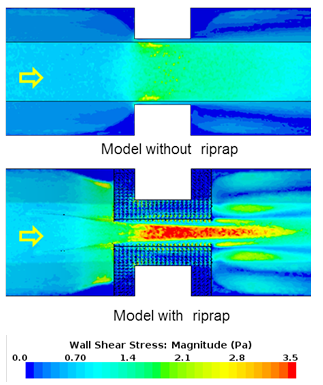
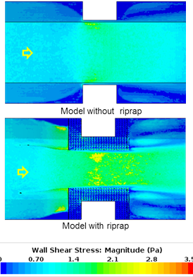
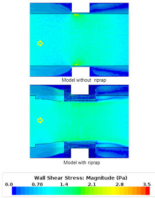
Figure 82 compares the bed shear stress distributions of the model with riprap with those of the model without riprap for case 11. In this case, the shear stress for the case without riprap, τB, was 0.029 lbf/ft2 (1.4 Pa), while the shear stress for the case with riprap, τR, was 0.070 lbf/ft2 (3.3 Pa). The shear ratio τR / τB is 2.4. Similarly, figure 83 and figure 84 provide the comparison for increasingly lower contraction ratios. The shear ratios for these cases dropped to 1.4 and 1.1, respectively.
 1 lbf/ft2 = 47.88 Pa. |
| Figure 82. Graphics. Comparison of bottom shear stress distribution for case 11. |
 1 lbf/ft2 = 47.88 Pa. |
| Figure 83. Graphics. Comparison of bottom shear stress distribution for case 13. |
 1 lbf/ft2 = 47.88 Pa. |
| Figure 84. Graphics. Comparison of bottom shear stress distribution for case 15. |
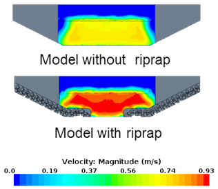
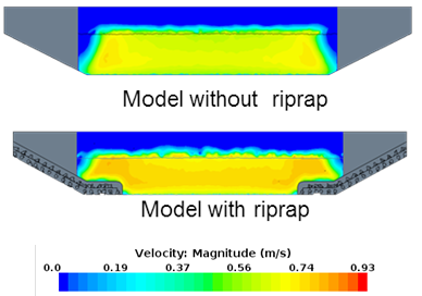
Figure 85 shows the velocity distribution for case 11. In this case, the apron for the model with riprap covered a significant part of the bottom, resulting in higher velocities compared with the model without riprap. As the opening became wider compared with the depth for case 13 (figure 86) and case 15 (figure 87), the difference between the model with riprap and the model without riprap diminished.
 1 lbf/ft2 = 47.88 Pa. |
| Figure 85. Graphics. Comparison of velocity distribution for case 11. |
 1 lbf/ft2 = 47.88 Pa |
| Figure 86. Graphics. Comparison of velocity distribution for case 13. |
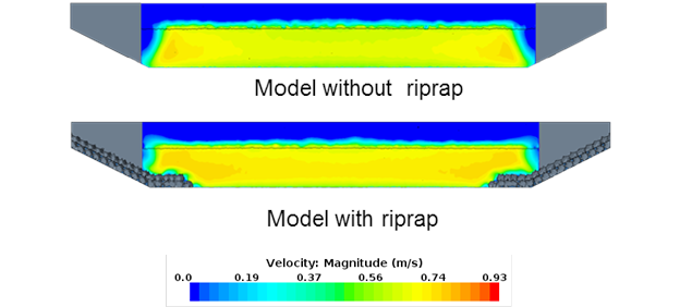 1 lbf/ft2 = 47.88 Pa |
| Figure 87. Graphics. Comparison of velocity distribution for case 15. |
Comparing the shear ratio of different groups in table 5, it can be seen that the shear ratio increased with the riprap size. For example, the shear ratios for three cases of the same W2/y0=6.2 increased from 1.27 for case 1, to 1.51 for case 6, and to 2.40 for case 11. The difference gradually decreased with increasing opening-to-width ratio, which indicated that the riprap size had a significant effect in narrower openings. The shear ratio almost doubled from case 1 to case11, but it was only 10 percent higher comparing case 5 to case 15. This phenomenon was mainly attributed to two reasons: 1) the near-bed secondary turbulence was increased owing to the larger roughness coefficient of larger riprap, and 2) riprap of larger size occupied more cross-sectional area in the opening assuming the contraction scour depth equals to two times D50. Results from full-scale CFD models showed the same trend as was observed for the laboratory-scale CFD tests.
Figure 88 summarizes the shear ratio data as a function of the ratio of W2/y0. As expected, the shear ratio decreased as the opening ratio increased within each group. Comparing across groups, those groups with larger riprap tended to have higher shear ratios as can be seen by comparing group 4 with group 1.
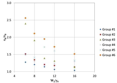 |
| Figure 88. Graph. Relationship between the opening-depth ratio and shear ratio. |
Returning to the conceptual equation shown in figure 55, the form of the equation appeared to validate the CFD modeling results. That equation also included a parameter, ε, which was not determined in chapter 3. However, using the CFD modeling results, a curve-fitting process was conducted based on the least squares method to determine the function ε. Values for the head loss coefficients, CcB and Cce, were assumed constant and equal to 0.23 for this exercise. Using these coefficients, equilibrium values of y2 and y2R were determined through iterative computations. (Alternatively, the depth values from the CFD modeling could have been used to determine the head loss coefficients, but the study did not have the resources to investigate this approach.) Figure 89 provides the resulting function.
![]()
Figure 89. Equation. Epsilon relation.
Figure 90 and figure 91 display the relationship between shear ratios and opening-to-depth ratios for the laboratory-scale and full-scale cases, respectively. For the laboratory-scale models, the Manning’s n ratio (nR/nB) increases from group 1 to group 2 to group 3 with values of 1.7, 1.8, and 1.9, respectively. Similarly, for the full-scale models, the Manning’s n ratio increases from group 4 to group 5 to group 6 with values of 2.0, 2.1, and 2.3, respectively. As expected, higher Manning’s n ratios resulted in higher shear ratios. The approach section Froude numbers for all cases were fairly consistent, ranging from 0.25 to 0.29. The contraction ratios (W2/W1) ranged from 0.72 to 0.90.
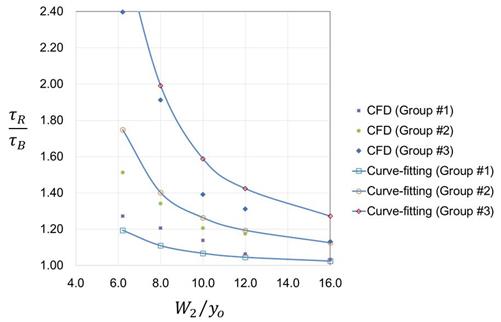
Figure 90. Graph. CFD results and curve-fitting for the laboratory-scale models.
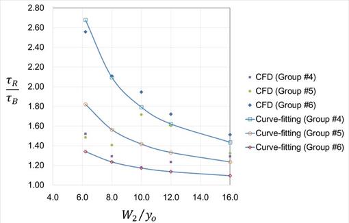
Figure 91. Graph. CFD results and curve-fitting for the full-scale models.
The estimated curves using the fitted equation in figure 55 for three groups were plotted against CFD results to verify that equation’s accuracy. The curve-fitting showed reasonable agreement with the results from CFD modeling for all groups. An exception to this observation for the laboratory-scale results was that the curves significantly underestimated values for W2/y0 equal to 6.2 and 8.0 for group 1 while overestimating the values for groups 2 and 3. A similar pattern was seen for the full-scale results.
Table 4 summarized the defining parameters for the buried installation cases in group 7 (cases31–35) including the geometry, riprap size, bed material size, and hydraulics, and table 5 summarized the shear stress and other results for these cases. Figure 92 provides an example of the results with a comparison of the bottom shear distributions between the condition with and without the riprap apron for case 33. In this case, the shear ratio was less than 1. The other cases in this group all had low shear ratios, with the largest ratio (1.08) being for case 34. With the exception of only two cases in group 1, all of the shear ratios for the buried installation (group 7) were smaller than for the cases for a flush installation (groups 1–6).
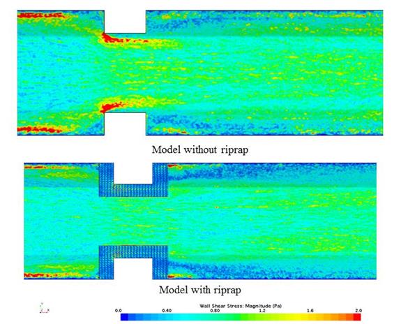 1 lbf/ft2 = 47.88 Pa. |
| Figure 92. Graphics. Comparison of bottom shear stress distribution for case 33. |
Burying the riprap appeared to significantly reduce or eliminate the increased shear in the unprotected channel caused by the flush installation of riprap aprons. To evaluate the possible reasons for this performance, it was useful to revisit the relation describing the shear ratio in figure 55. The variables potentially influencing the shear ratio included the roughness ratio, the width ratio, W2/y0, the vertical adjustment ratio, ΔZ/y1, and the approach flow Froude number. The effect of the Froude number, if any, depended on the channel shape factors.
Figure 93 displays a plot of the shear ratio for the six flush installation groups and the one buried installation group versus Manning’s n ratio. Although group 7 had the largest Manning’s n ratio, the data from that group did not align at all with the other groups. Similarly disjointed results were observed when examining Froude number.
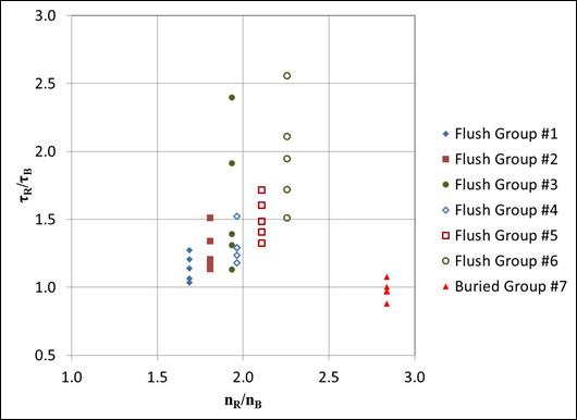 |
| Figure 93. Graph. Shear ratio compared with Manning’s n ratio. |
Figure 94 displays a plot using the same cases of the shear stress ratio versus the vertical adjustment ratio. In this case, the group 7 data were consistent with the general trends of other groups, with the lowest set of shear ratios corresponding to the lowest set of vertical adjustment ratios. In this graph, increasing vertical adjustment ratio implies increasing shear ratio.
The vertical adjustment parameter, Δ Z, was defined in figure 44. It represented the average blocked area flush installation of riprap within the contraction scour zone. The larger this number was, the greater the blockage. If the vertical adjustment parameter was 0, as it was with the group 7 data, there was no blockage and contraction scour was unhindered. Recall that the buried riprap was intended to be located below the contraction scour zone.
The previous discussion regarding the flush installation noted the general decline in shear ratio with respect to increasing contracted width, W2, as shown in figure 88, for example. This was true because the vertical adjustment dropped with increasing contracted width. Therefore, the primary mechanism for the shear ratio was the blockage of conveyance in the contraction scour zone by the flush installation of riprap. Buried installation below the contraction zone eliminated this problem.
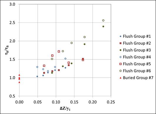 |
| Figure 94. Graph. Shear ratio compared with vertical adjustment ratio. |
Table 6 summarizes the defining parameters for each case, including geometry, bed material size, and hydraulics for the alternative setback cases. All of these cases were without riprap. The cases with alternative setbacks can be compared with the group 7 cases 32–35.
| Group | Case | Bed D50 (inches) |
W1 (ft) |
y1 (ft) |
A1 (ft2) |
V1 (ft/s) |
W2 (ft) |
y0 (ft) |
y2 (ft) |
V2 (ft/s) |
|---|---|---|---|---|---|---|---|---|---|---|
| Short extension slope | 36 | 0.04 | 78.35 | 9.68 | 570.9 | 2.02 | 49.87 | 6.23 | 9.68 | 2.46 |
| 37 | 0.04 | 90.81 | 9.68 | 691.6 | 2.10 | 62.34 | 6.23 | 9.68 | 2.46 | |
| 38 | 0.04 | 103.28 | 9.68 | 812.3 | 2.15 | 74.80 | 6.23 | 9.68 | 2.45 | |
| 39 | 0.04 | 128.22 | 9.68 | 1053.6 | 2.21 | 99.74 | 6.23 | 9.68 | 2.45 | |
| Long extension slope | 40 | 0.04 | 72.11 | 9.68 | 510.6 | 2.16 | 49.87 | 6.23 | 9.68 | 2.45 |
| 41 | 0.04 | 84.58 | 9.68 | 631.3 | 2.21 | 62.34 | 6.23 | 9.68 | 2.45 | |
| 42 | 0.04 | 97.05 | 9.68 | 751.9 | 2.25 | 74.80 | 6.23 | 9.68 | 2.44 | |
| 43 | 0.04 | 121.98 | 9.68 | 993.3 | 2.29 | 99.74 | 6.23 | 9.68 | 2.44 | |
|
1 inch = 25.4 mm. 1 ft = 0.305 m. 1 ft2 = 0.093 m2. 1 ft/s = 0.305 m/s. |
||||||||||
Table 7 summarizes the shear stress on the bed material and other results from the runs. The effect of the channel setback on contraction shear stress may be compared for each value of W2/y0. For W2/y0 equal to 8, cases 32, 36, and 40 were compared. For W2/y0 equal to 10, cases 33, 37, and 41 were compared. Similar comparisons were made for W2/y0 equal to 12 and 16. For each W2/y0, the parameters of y2, W2, V2, and y1 were held constant, while the setback was increased. Increasing the setback reduced W1 and increased W2/W1, effectively reducing the contraction from the approach to the bridge opening. Because the hydraulic conditions in the contraction itself were the same, but the flow contraction from the approach was reduced, the shear stress, τB, generally decreased with increasing setback. This result was expected.
| Group | Case | Equivalent W1 (ft) |
W2 / y0 | Fr1 | τB (lbf/ft2) |
nB | W2 / W1 | |||
|---|---|---|---|---|---|---|---|---|---|---|
| Short extension slope | 36 | 58.99 | 8.0 | 0.11 | 0.0203 | 0.013 | 0.85 | |||
| 37 | 71.46 | 10.0 | 0.12 | 0.0144 | 0.013 | 0.87 | ||||
| 38 | 83.92 | 12.0 | 0.12 | 0.0175 | 0.013 | 0.89 | ||||
| 39 | 108.86 | 16.0 | 0.13 | 0.0138 | 0.013 | 0.92 | ||||
| Long extension slope | 40 | 52.76 | 8.0 | 0.12 | 0.0167 | 0.013 | 0.95 | |||
| 41 | 65.22 | 10.0 | 0.13 | 0.0230 | 0.013 | 0.96 | ||||
| 42 | 77.69 | 12.0 | 0.13 | 0.0161 | 0.013 | 0.96 | ||||
| 43 | 102.62 | 16.0 | 0.13 | 0.0144 | 0.013 | 0.97 | ||||
|
1 ft = 0.305 m. 1 lbf/ft2 = 47.88 Pa |
||||||||||
However, some shear stress values increased with increasing setback, (e.g., comparing case 41 with case 37. The approach velocity, V1, also increased with increasing setback for a given W2/y0 ratio. The conflicting trends of increasing approach velocity and decreasing contraction might explain the inconsistent trend in shear stress.
Another observation pertains to the shear stress at the upstream corner of the abutment that results in abutment (local) scour. As can be seen in the shear stress figures in appendix C, increasing setback length reduced the shear stress that caused abutment scour.