U.S. Department of Transportation
Federal Highway Administration
1200 New Jersey Avenue, SE
Washington, DC 20590
202-366-4000
Federal Highway Administration Research and Technology
Coordinating, Developing, and Delivering Highway Transportation Innovations
| REPORT |
| This report is an archived publication and may contain dated technical, contact, and link information |
|
| Publication Number: FHWA-HRT-17-013 Date: February 2017 |
Publication Number: FHWA-HRT-17-013 Date: February 2017 |
One hypothesis for this research effort was that the use of riprap aprons installed flush with the bed in some bridge openings might increase the depth of contraction scour within the opening between the riprap aprons. In this chapter, a conceptual model illustrating the basis for this hypothesis is developed.
Figure 2 shows a simplified plan view of a river channel with bridge abutments encroaching into the channel. Riprap aprons are also shown as a protection against abutment scour. The hypothesis was that the presence of these aprons for abutment scour had the potential to increase contraction scour in the area of the channel in the unprotected gap between the aprons. The relevant hydraulic parameters are also shown in the figure, including the upstream velocity (V1,), velocity in the abutment opening (V2), riverbed bottom width upstream (W1), the bridge opening (W2), the flow depth upstream (y1), abutment length (l1), and abutment width (l2).
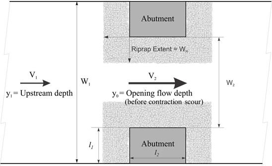 WR = Riprap apron width. |
| Figure 2. Sketch. Plan view of a bridge contraction with riprap apron. |
Figure 3 shows a schematic of a simple bridge opening (contraction) without a riprap apron. As previously defined, W1 is the bottom width of the upstream (approach) channel, and W2 is the bottom width of the contracted (bridge) opening. The average contraction scour in the bridge opening is yc.
This study focused on vertical-wall abutments, as shown in figure 3. These abutments take many forms, including GRS abutments placed on RSFs. This type of abutment and foundation is considered a non-rigid foundation. According to design guidance in HEC-23, the top of the abutment foundation should be located at the lower extent of the estimated contraction scour and LTD.(3) LTD was negligible in the physical modeling because equilibrium conditions were used.
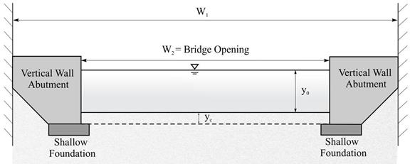 |
| Figure 3. Sketch. Cross section of pre-scour condition for case without riprap. |
Figure 4 shows the contracted bridge opening with the riprap apron to protect the abutment foundation from abutment scour as specified in HEC-23. (3)The apron width, WR, is extended from the abutment face a distance equal to twice the pre-scour flow depth in the opening, y0. The recommended apron thickness, according to HEC-23, is 1.5×D50 or D100 (the maximum rock size), whichever is greater. It is shown in the figure from the pre-scour bed elevation to the top of the foundation.(23)
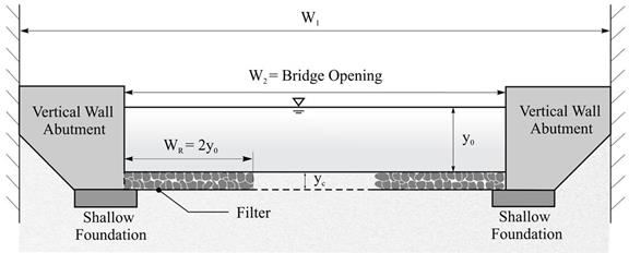 |
| Figure 4. Sketch. Cross section of pre-scour condition for case with riprap. |
When the contraction scour for the situation shown in figure 3 occurred, a shear stress remained on the bed material. If this was the equilibrium contraction scour depth, the shear stress would equal the critical shear stress for the bed material. To generalize, that shear stress on the bed without riprap aprons was referred to in this study as τB. Similarly, when the same contraction scour shown in figure 4 occurred but with riprap aprons present, that shear stress was defined in this study as τR. Although both shear stresses were considered at the same depth (y0 + yc), the hypothesis of this study was that the presence of the riprap caused τR to exceed τB so that further contraction scour would occur for the case with riprap.
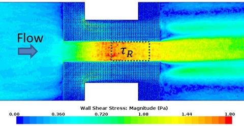
Numerical CFD modeling, which is discussed in chapter 5, supported this hypothesis. Figure 5 shows the bed shear stress distribution for a case without riprap after contraction scour occurred. In the region of interest, the value of τB was approximately 0.023 lbf/ft2 (1.1 Pa). Figure 6 displays the bed shear stress distribution at the same level of scour for the same contraction geometry, but with riprap aprons. In the same region of interest, the shear stress was higher, such that τR was approximately 0.031 lbf/ft2 (1.5 Pa). The difference between the two values depended on the specific circumstances of the contraction and riprap characteristics. The shear ratio τR/τB was used as an index to evaluate the influence induced by a riprap installation.
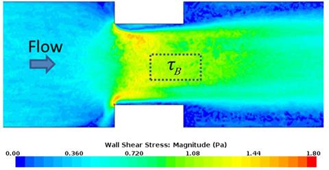 1 lbf/ft2 = 47.88 Pa. |
| Figure 5. Graphic. Numerically modeled shear stress distribution for case without riprap. |
 1 lbf/ft2 = 47.88 Pa. |
| Figure 6. Graphic. Numerically modeled shear stress distribution for case with riprap. |
A dimensional analysis was used to better understand the relationship between the ratio of shear with and without riprap abutment protection to potential independent variables. The general equations for the case without riprap and with riprap are shown in figure 7 and figure 8, respectively.
![]()
Figure 7. Equation. Relevant variables for case without riprap.
![]()
Figure 8. Equation. Relevant variables for case with riprap.
Where:
ρ = Water density (lb/ft3 (kg/m3)).
g = Acceleration resulting from gravity (ft/s2 (m/s2)).
μ = Viscosity (lbf∙s/ft2 (N s/m2)).
These equations can be expressed as ratios, normalizing using the upstream hydraulic variables and water density, as shown in figure 9 and figure 10.
![]()
Figure 9. Equation. Normalized variables for case without riprap.
![]()
Figure 10. Equation. Normalized variables for case with riprap.
These relations can be reduced further by recognizing the following:
With these observations, the cases without and with riprap are summarized in figure 11 and figure 12, respectively.
![]()
Figure 11. Equation. Reduced function for case without riprap.
![]()
Figure 12. Equation. Reduced function for case with riprap.
Conversion of these equations to a formulation expressing the shear is shown in figure 13 and figure 14 for the cases without and with riprap, respectively.
![]()
Figure 13. Equation. Shear function for case without riprap.
![]()
Figure 14. Equation. Shear function for case with riprap.
Where:
Fr = Froude number (dimensionless).
Re = Reynolds number (dimensionless).
Then, the ratio of shear stress with riprap to the case without riprap can be written as shown in figure 15.
![]()
Figure 15. Equation. Shear ratio of case with riprap to case without riprap.
The Reynolds number (Re) is defined as the ratio of inertial forces to viscous forces and consequently quantifies the relative importance of these two types of forces. For this application, Re was not important because the bed shear primarily depended on the local velocity gradient on the bed.
Further, if a constant abutment length was assumed, the term with l1 was not needed. Dropping the terms with Re and l1 yielded the formulation shown in figure 16.
![]()
Figure 16. Equation. Final shear ratio of case with riprap to case without riprap.
Where:
∅ = Undefined function.
The specific functional formulation expressing the ratio of τR / τB was derived from the continuity, energy, and momentum equations comparing the situations with and without riprap aprons.
Figure 17 provides a conceptual definition sketch of the approach (upstream) section and contracted (bridge opening) section for the case where there is no riprap. To simplify the numerical modeling with CFD, an alternative definition sketch was used, as shown in figure 18. The change from the conceptual definition was to alter the upstream section so that the bottom elevation was increased by the estimated contraction scour depth, yc.
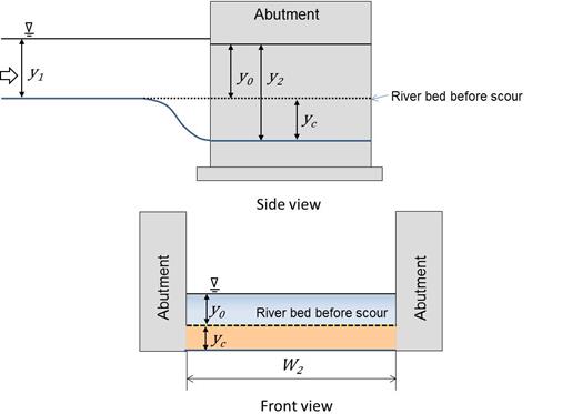 |
| Figure 17. Sketch. Conceptual schematic for case without riprap. |
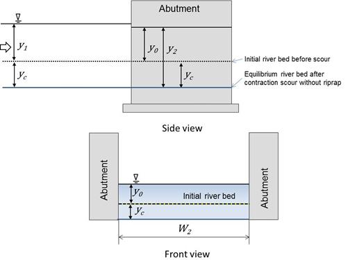 |
| Figure 18. Sketch. CFD schematic for case without riprap. |
The flow condition in the opening without riprap at equilibrium contraction scour is shown in figure 19. For this case, the bottom roughness for the natural bed material is nB and the average shear stress on the bed is τB.
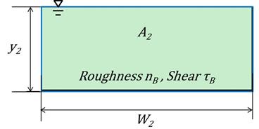 |
| Figure 19. Schematic. Cross section in the opening for case without riprap. |
Figure 20 displays a schematic consistent with the CFD analysis for use with the continuity and energy equations. The variable ŷ1 is equal to y1 + yc, as shown in figure 18.
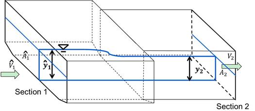 Â1 = Cross-sectional area of upstream section for CFD experiments. ŷ1 = Average flow depth in upstream section for CFD experiments. y2 = Average flow depth in contracted section with riprap after contraction scour. A2 = Cross-sectional area of contracted section without riprap at equilibrium contraction scour. |
| Figure 20. Schematic. Continuity and energy control volume for case without riprap. |
For the case without riprap, the continuity equation is summarized in figure 21, and the energy equation is summarized in figure 22.
![]()
Figure 21. Equation. Continuity equation for case without riprap.
![]()
Figure 22. Equation. Energy equation for case without riprap.
Where:
z1 = Reference elevation for upstream section (ft (m)).
z2 = Reference elevation for downstream section (ft (m)).
α1 = Energy correction factor for upstream section (dimensionless).
α2B = Energy correction factor for contracted section without riprap (dimensionless).
hB = Head loss between upstream section and contracted section without riprap (ft (m)).
The energy correction factors were approximately equal to 1.00 to 1.01 for gradually varied flow. The head loss between to the two sections without riprap, hB, is defined as the contraction coefficient without riprap, CcB, times the velocity head in the contracted section. Therefore, the equation in figure 22 was modified to the equation in figure 23 assuming that the two reference elevations were approximately equal (mild slope) and substituting for V2 from the continuity equation.
![]()
Figure 23. Equation. Modified energy equation for case without riprap.
Where:
CcB = Contraction coefficient for model without riprap (dimensionless).
The quantity in brackets is defined in figure 24 as the channel shape factor for the case withoutriprap.

Figure 24. Equation. Channel shape factor for case without riprap.
Where:
βB = Channel shape factor for model without riprap (dimensionless).
Substituting the channel shape factor yielded the equation in figure 25.
![]()
Figure 25. Equation. Flow depth ratio for case without riprap.
Where:
![]() 1 = Froude number for CFD experiments, which is defined as
1 = Froude number for CFD experiments, which is defined as ![]() (dimensionless).
(dimensionless).
An equation for shear stress was also required, as shown in figure 26.
![]()
Figure 26. Equation. Average bed shear stress for case without riprap.
Where:
S = Energy slope (ft/ft (m/m)).
γ = Unit weight of water (lbf/ft3 (N/m3)).
Using Manning’s equation, as shown in figure 27, and assuming relatively smooth walls so that the hydraulic radius can be approximated as area divided by width (A/W) yielded the equation given in figure 28.
![]()
27. Equation. Manning’s equation for case without riprap.
Where:
nB = Roughness coefficient for bed material (dimensionless).
Rh = Hydraulic radius (ft (m)).

Figure 28. Equation. Bed shear for case without riprap.
The same application of the continuity, energy, and momentum equations was applied to the case with riprap. Figure 29 provides a conceptual definition sketch of the approach (upstream) section and contracted section for the case where there was riprap. The flow depth at equilibrium scour, y2R, is shown as greater than the flow depth at equilibrium without the riprap, y2. As for the case without riprap, to simplify the numerical modeling with CFD, an alternative definition sketch was used, as shown in figure 30. The change from the conceptual definition was to alter the upstream section so that the bottom elevation was increased by the estimated contraction scour, yc.
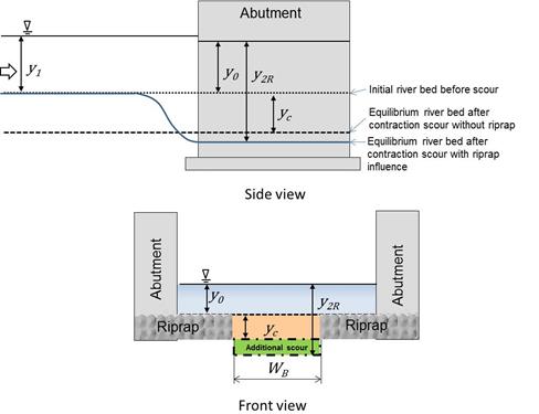 WB = Bottom width of bed material. |
| Figure 29. Sketch. Conceptual schematic for case with riprap. |
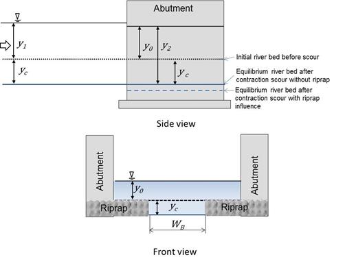 |
| Figure 30. Sketch. CFD schematic for case with riprap. |
The flow condition in the opening with riprap at the estimated contraction scour without riprap (y2=y0 + yc) is shown in figure 31. For this case, the bottom roughness for the natural bed material was nB, and the bottom roughness for the riprap was nR.
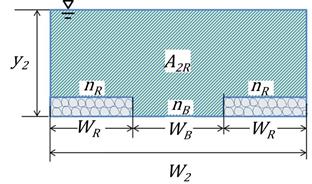 A2R = Cross-sectional area of contracted section with riprap after contraction scour to a depth of yc. |
| Figure 31. Schematic. Cross section in the opening for case with riprap. |
Figure 32 displays a schematic consistent with the CFD analysis for use with the continuity and energy equations. The variable ŷ1 was equal to y1 + yc, as shown in figure 30.
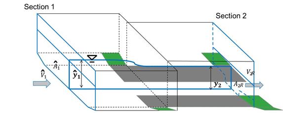 |
| Figure 32. Schematic. Continuity and energy control volume for case with riprap. |
For the case with riprap, the continuity equation is summarized in figure 33, and the energy equation is summarized in figure 34.
![]()
Figure 33. Equation. Continuity equation for case with riprap.
![]()
Figure 34. Equation. Energy equation for case with riprap.
Where:
V2R = Average velocity in contracted section with riprap after contraction scour to a depth of yc (ft/s (m/s))
α2R = Energy correction factor for contracted section with riprap (dimensionless).
hR = Head loss between upstream section and contracted section with riprap (ft (m)).
The energy correction factors were approximately equal to 1.00 to 1.01 for gradually varied flow. The head loss between to the two sections, hR, was defined as the contraction coefficient for the model without riprap, CcR, times velocity head in the contracted section. The equation in figure 34 was modified to the equation in figure 35 assuming that the two reference elevations were approximately equal (mild slope) and substituting for V2 from the continuity equation.
![]()
Figure 35. Equation. Modified energy equation for case with riprap.
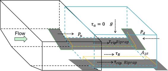
To develop a relation for shear stress at the bed after contraction scour had reached a depth of y2, two assumptions were made. First, it was assumed that flow in the contraction could be characterized as gradually varied flow. From this, it followed that the flow acceleration was approximated as 0, and the difference between the upstream pressure and the downstream pressure, Pu – Pd, was also approximately 0. Second, it was assumed that the front faces of abutment were smooth. From this, the shear on the front face of abutment, τa, was approximately 0. These quantities are shown on the control volume schematic in figure 36.
 τrip = Average bed shear stress on riprap. |
| Figure 36. Schematic. Momentum control volume for case with riprap. |
The average bed shear for the case with riprap in the contraction is shown in figure 37.
![]()
Figure 37. Equation. Bed shear stress for case with riprap.
The average bed shear in the opening is expressed in figure 38.
![]()
Figure 38. Equation. Average bed shear stress for case with riprap.
By substituting the equation in figure 38 into the equation in figure 37, an expression for the energy slope was derived, as shown in the equation in figure 39.
![]()
Figure 39. Equation. Energy slope for case with riprap.
Manning’s formula in the open channel with composite roughness, n, is written as shown in figure 40.
![]()
Figure 40. Equation. Manning’s equation for case with riprap.
Assuming relatively smooth abutment walls and neglecting the vertical sides of the riprap, the hydraulic radius could be approximated as A2R/W2. Substituting the equation in figure 39 into the equation in figure 40 yields the expression shown in figure 41 for average bottom shear stress.

Figure 41. Equation. Bed shear for case with riprap.
The composite Manning’s roughness coefficient, n, can be calculated using the composite roughness formula shown in figure 42.(21,22)

Figure 42. Equation. Composite n.
Composite n for the bed and riprap materials was calculated using Strickler’s equation, which relates roughness coefficient to the size of bed material.(23) Following the HEC-23 design guidance, the apron width, WR, was specified as 2y0. Expressing the natural bed width in terms of W2 led to the representation of composite n in figure 43.(3)

Figure 43. Equation. Composite n in terms of depth and width.
The section in figure 31 for the riprap case was simplified to the equivalent rectangular cross section shown in figure 44. The equivalent depth, ye, plus the vertical adjustment, Δ Z, was equal to y2. The bed had a composite roughness, n, and an average bed shear stress of τavg. The cross-sectional area was the same as it was for the previous riprap case.
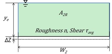 |
| Figure 44. Schematic. Equivalent opening cross section with uniform roughness and shear. |
Figure 45 illustrates the control volume for the equivalent depth case with riprap. The energy equation for this case is shown in figure 46.
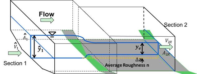 |
| Figure 45. Schematic. Control volume for the equivalent depth with riprap. |
![]()
Figure 46. Equation. Energy equation for equivalent depth case with riprap.
Assuming a mild slope where z1 was approximately equal to z2 and taking the energy correction factors α2R and α2e as equal to 1.0 led to the equation shown in figure 47.
![]()
Figure 47. Equation. Modified energy equation for equivalent depth case with riprap.
Where:
Cce = Contraction coefficient for equivalent model with riprap (dimensionless).
Defining the channel shape factor, βe, as shown in figure 48, and rewriting the equation in figure 47 in terms of a depth ratio led to the equation in figure 49.
![]()
Figure 48. Equation. Channel shape factor for equivalent depth case with riprap.
![]()
Figure 49. Equation. Depth ratio for equivalent depth case with riprap.
Where:
Βe = Channel shape factor for equivalent model with riprap (dimensionless).
The ratio of bed shear for the case with riprap (figure 41) to the one without riprap (figure 28) is shown in figure 50.

Figure 50. Equation. Shear stress ratio.
Using the expression for composite n in figure 43, the ratio of roughness values is shown in the equation in figure 51.

Figure 51. Equation. Manning’s roughness ratio.
The area ratio in figure 50 can be expressed in terms of depth. Because A2 was equal to W2 times y2 (figure 19), and A2R was equal to W2 times ye (figure 44), the area ratio is represented as shown in figure 52.
![]()
Figure 52. Equation. Area ratio.
Substituting the roughness ratio in figure 51 and the area ratio in figure 52 into the equation in figure 50 led to the shear stress ratio in figure 53.

Figure 53. Equation. Shear stress ratio with substitutions.
Further substitution for y2 (figure 25) and ye (figure 49) led to the equation in figure 54.

Figure 54. Equation. Shear stress ratio with average shear stress.
Where:
![]() = Froude number for CFD experiments, which is defined as
= Froude number for CFD experiments, which is defined as ![]() (dimensionless).
(dimensionless).
On the left side of the equation, τavg was replaced with τR, and on the right side, the exponent of 4/3 was replaced by a new parameter, ε, as shown in figure 55. A relation for estimating ε was explored by evaluating the CFD analytical results.

Figure 55. Equation. Shear stress ratio with τR
Where:
ε = Function related to ratio of roughness of riprap to that of erodible bed material (dimensionless).
As is apparent from the equation in figure 55, the ratio of the shear stress in the middle of the channel with and without the riprap aprons varied with several factors. The relative size of the riprap relative to the bed material was expressed in the ratio of the Manning’s roughness values, nR/nB. The flow dimensions in the contraction were expressed in the ratio of the contraction width to the flow depth before scour. A high value of this ratio could be considered a wide channel, and a low value might be called a narrow channel. In addition, the degree of contraction, including energy losses, was included in the term in the equation that included the channel shape factors. The extent of contraction would also influence the size of riprap required for abutment protection. This shear ratio was investigated with the CFD modeling described in chapter 5.