U.S. Department of Transportation
Federal Highway Administration
1200 New Jersey Avenue, SE
Washington, DC 20590
202-366-4000
Federal Highway Administration Research and Technology
Coordinating, Developing, and Delivering Highway Transportation Innovations
| REPORT |
| This report is an archived publication and may contain dated technical, contact, and link information |
|
| Publication Number: FHWA-HRT-13-097 Date: September 2014 |
Publication Number: FHWA-HRT-13-097 Date: September 2014 |
Built Environment
The potential influence of the built environment on travel behavior has been widely studied in the literature.(56,67,68) Early studies of land use and travel behavior focused more on hypothesis testing regarding the correlation between built environment and travel, but the debate about causality of observed correlations is ongoing. Despite the large number of existing studies, the magnitude of the effects of built environment on travel behavior, specifically mode choice, is unclear. Self-selection/endogeneity and serial and spatial correlation among individuals and environments surveyed are difficult to measure and evaluate, and the relationships between built environment and travel behavior cut across levels of time and space.
Cao et al. and Mokhtarian and Cao provide an extensive discussion on how to robustly infer causality in this regard.(8,9) To do so, four types of evidence are required: correlation, non-spuriousness, time precedence, and causal mechanism.(9) Correlation refers to a significant association between the considered variables and travel behavior. Non-spuriousness refers to a relationship that cannot be attributed to another variable. Time precedence requires causes to precede effects, and causal mechanism is a logical explanation for why a cause should produce the observed effect. Many studies in the past have carefully controlled for the statistically significant correlations and causal mechanism in which a logical explanation of the cause and effect exists. However, few studies have been able to meet the non-spuriousness and time precedence criteria.(69) Mokhtarian and Cao suggested that a model that explicitly includes attitudinal and socio-demographic variables could perform well on the non-spuriousness criterion, specifically with regard to residential self-selection.(9) “Residential self-selection” refers to the tendency of people to choose locations based on their travel abilities, needs and preferences.(69) Therefore, an observed correlation between land use and travel behavior can be ensured to be the non-spurious result of the unmeasured variables. Performing temporal analyses and involving measurement at multiple points in time can help to meet the time precedence criterion.(9,70) While these considerations would help strengthen a planner’s argument, they still fall short of accepted standards for scientific evidence.
Most of the land use-travel behavior studies are regression-based, in which socio-demographic characteristics and measures of land use are treated as independent variables.(69) Suggesting that the underlying behavioral structure of how land use influences travel is missing in regression-based analyses, Boarnet provided a review of methodologies to overcome this limitation.(71) Land use can influence the cost to travel by changing travel time. Boarnet and Crane suggested that travel speed and trip distance are functions of land use and proposed using a composite travel price variable representing the impact of land use on travel cost.(26) Cervero also uncovered the possible impacts of residential self-selection on travel behavior.(72) A quantitative approach suggested by some researchers to deal with this problem is to develop joint discrete choice models of residential location and travel behavior.(73–75) The endogeneity of policies, plans, and urban development patterns is another limitation which has been virtually neglected in the literature.(71,76) This endogeneity results in serial and spatial correlation, which affects how individuals make decisions over time, affecting network accessibility and location choices.
A recent study by Zhang analyzed the influence of land use on travel mode choice using data from Boston, MA, and Hong Kong for work and non-work travel.(68) Under the assumption that attitudes affect both travel behavior and land use through residential self-selection, this study did not properly detect the true effect of land use on mode choice because the model did not consider self-selection bias. Improvement in a model’s goodness-of-fit after the inclusion of land use variables does not necessarily imply that land use has an independent influence on mode choice.(68)
Crime
While transit agencies can control many aspects of their service, the public nature of transit means that passengers’ experienced quality of service is subject to environmental factors often outside of the agency’s control. Concern for personal safety/security is a primary concern of transit riders and non-riders, and studies suggest that fear of crime acts as a deterrent to transit ridership. (See references 77–80.) Needle and Cobb presented case studies that indicated that crime and peoples’ perception of it reduces transit ridership and revenues.(81)
Loukaitou-Sideris et al. studied 10 bus stations with the highest crime rates in Los Angeles, CA, and found that physical environment and the occurrence of crime are correlated.(79) Most of the 10 high-crime bus stops in the study were located in parts of the city that lack proper lighting, good police deployment, or public phones (the study precedes the widespread availability of mobile phones). Painter studied the effects of street lighting on crime, fear of crime, and pedestrian street use and also concluded that lighting improvements can reduce street crimes to a large extent.(82) Painter also found that street lighting could increase pedestrians’ propensities to use the streets after dark in urban streets and residential settings.(82) One approach to reduce crime at transit stations is to follow recommendations of a program called Crime Prevention Through Environmental Design (CPTED).(83,84) The CPTED concept is based on the defensible space concept in which people need to see and be seen in order to protect themselves and avoid crime, and people need to report crimes when they occur.
Some studies have suggested counterintuitive results (i.e., higher crime attracts transit use). This may be because crime influences market segments differently. Transit captives by definition do not have much choice in mode, so the interaction of crime and income and their effects on transit use is still unclear. Ferrell and others have argued that these contradictory results of effects of crime on women and adolescents’ physical activities could be related to the differences in actual/reported crimes and individual perceptions of neighborhood crime.(85,86) Less serious crimes such as intimidation, public indecency, obscenities, vagrancy, and vandalism affect the transit environment but may go unreported if riders choose to ignore them. While in these studies the relationship between reported crimes and physical activity engagement is unclear, the perceptions of crime and safety are related to the physical activity engagement.(87) Kim et al. found that women’s access mode to transit is influenced by crime. Women are more likely to be dropped off at the station at night than drive, use transit, or walk.(88) Employing CPTED concepts to enhance defensibility, awareness, and surveillance could influence these choices over time.
Behavioral Dimensions—Mode Choice
Cervero and Kockelman suggested that land use characteristics can be categorized in “three D’s:” density, diversity, and design.(52) Density refers to the variable of interest divided by area (e.g., population density, job density, etc.). Diversity refers to the different land uses in a given area (e.g., entropy index, diversity index, mixed use development, etc.). Design refers to the properties of the network such as connectivity, grid, or cul-de-sac, etc. Zhang summarized the direction of effects of land use on travel behavior (see table 1).(68) An increase in density often decreases the likelihood of driving, driving length, and trip chaining while having mixed effects on driving frequency, route choice, and telecommuting. Increases in diversity measures reduces driving choice while increasing driving frequency and trip chaining. Diversity has mixed effects on driving length and route choice. Network design with more connectivity also decreases the likelihood of driving while it may increase driving frequency. The effects of land use on departure time choice and telecommuting are mostly unknown.
Table 1. Summary of the effects of land use on travel behavior.(68)
| Travel Behavior | Dimensions of Land Use | Travel Patterns | ||
| Density | Diversity | Design | ||
| Driving choice | - | - | - | Modal split |
| Driving frequency | ± | + | + | Total trips |
| Driving length and duration | - | ± | ? | VMT/vehicle hours traveled |
| Departure time | ? | ? | ? | Peaking |
| Route choice | ± | ± | ± | Road congestion |
| Trip chaining | - | + | ± | Trip rate and distance |
| Tele-travel | ± | ? | ? | All |
| Note: The symbols +, -, and ? indicate positive, negative, and unknown effects, respectively. | ||||
The research has grown from the “three D’s” to include detail, destination, and a dozen others. This requires new ways of thinking and additional data to understand a suite of trips and socialization. There are strong attitudinal elements and a wide variation of elasticity of attitudes with respect to different interventions; this requires capturing heterogeneity among travelers. The understanding of interactions between modes is growing, and often a number of modes are competing for the same space. There are also interactions between network and non-network characteristics of modes. For example, walkability requires that sidewalks exist and be in good condition. There is a demand for different products, so researchers need to think of a synergistic suite of options or a mobility bundle.
The FHWA Complete Streets program is intended to examine such mobility bundles and provide viable alternatives to auto travel via infrastructure that accommodates all types of users. The program suggests improving land use and design measures that enhance accessibility and walk quality, such as sidewalks, bicycle lanes, safe and accessible transit stops, and frequent and safe crossings for pedestrians.(89) Regarding transit accessibility, several studies have found a positive impact on transit choice with elasticities between 0.02 and 1. (See references 90−94.) Others have looked at the effect of transit accessibility on VMT. (See references 90, 92, and 95–99.) They all found a significant negative impact with elasticities between -0.01 to -0.19. Mixed use development has been found to have a positive impact on transit choice. Studies by Zhang and Frank et al. suggest that the effect of land use mix on transit choice is larger for non-work trips than work trips.(92) Table 2 presents point elasticities of different land use variables reported by Cervero.(56) Sidewalk ratio, as a walk quality measure, has a negative impact on driving regardless of trip purpose and positive impact on transit use.
Table 2 . Point elasticity estimates imputed from mode choice models: percentage change in
probability of choosing mode with a 1 percent increase in built environment factor.(56)
| Built-Environment | Home-Based Work Trips | All Trip Purposes | ||
| Drive Alone | Drive Alone | Group Ride | Transit | |
| Gross density1, origin | -0.151 | -0.163 | -0.124 | +0.511 |
| Gross density, destination | -0.259 | -0.137 | -0.096 | +0.268 |
| Land use diversity2, origin | -0.141 | -0.340 | -0.361 | +0.615 |
| Land-use diversity, destination | -0.197 | -0.291 | -0.165 | +0.452 |
| Sidewalk ratio3, origin | -0.390 | |||
| Sidewalk ratio, destination | -0.448 | -0.366 | -0.062 | +0.327 |
| Transit-oriented multi-family housing, origin | -0.052 | -0.066 | +0.195 | |
| Job accessibility4, origin | +0.141 | |||
| Labor force accessibility5, destination | +0.290 | |||
|
Note: Blank cells indicate instances that were not measured. |
||||
Framework for Evaluation
The interest in analyzing transport policies in terms of their impacts has led to the use of disaggregate demand models, which seek to understand short-term effects of such policies as congestion pricing. The limitation of traditional trip-based travel models to capture the complex ways travelers respond to such policies has led to the development of behavior-oriented activity-based models and the introduction of traveler response to current cost, travel time, reliability, and other service information.
The advantages of activity-based models are diverse and include the following:
These are also the main reasons to incorporate an activity-based framework over a trip- or tour-based framework into the analysis of pricing policies.
Within activity-based models, the modeled behavior choices for households and individuals are normally organized sequentially on the basis of the timeframe over which they might take place. Long-term decisions are modeled first, followed by medium- and short-term decisions. Each of the models imposes certain restrictions on the subsequential decisions on a shorter time horizon. The same conceptual framework is kept in place for integrating activity-based models with the network assignment procedure to analyze pricing strategies, which is discussed later in this report regarding traveler response to network information.
In the short term, it is expected that travelers’ safety/security perception and built environment factors influence mode choice. However, in the medium-to-long-term horizons where policy influences the environment and crime rates, policy will indirectly influence further user decisions. This is illustrated in figure 3 by taking accessibility measurement calculations into account, which in return have effects on upper-level choices of car ownership, daily activity patterns, as well as longer-term higher order choices of home, workplace, and school locations.
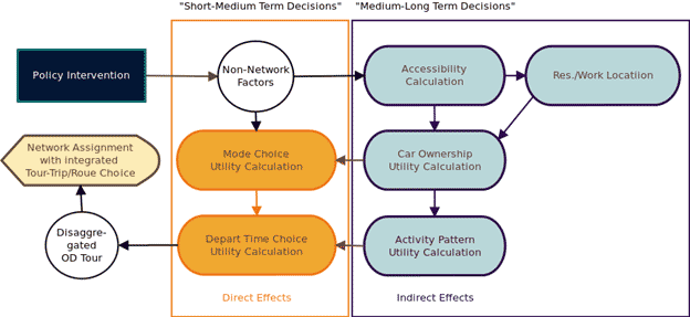
Figure 3. Illustration. Direct and indirect influences of non-network factors over time.
In order to detect the true effect of land use, Mokhtarian and Cao proposed different approaches including direct questioning, statistical control, instrumental variables modeling, sample selection modeling, joint models, and longitudinal designs.(9) Direct questioning refers to asking people in focus groups and personal interviews whether land use affects their travel behavior. The statistical method estimates the proportion of total effect of land use on travel behavior which is due to land use alone rather than due to the effect of attitudes on land use (via residential self-selection) by inclusion of a rich set of attitudinal and socio-demographic variables in the model. In instrumental variable models, land use is first modeled as a function of relevant instrumental variables and then replaced in the choice model. The sample selection modeling technique explicitly models the prior selection into different residential location types and then models the outcome as conditional on that prior selection. The joint modeling approach considers endogenous variables of residential location and travel behavior jointly and models the joint probability bundled. Finally, longitudinal design refers to before-after measurements. Referring back to the study by Zhang, although a significant correlation between land use and travel behavior was observed, the magnitudes of the elasticity estimates for mode choice with respect to the land use variables were relatively small, with an absolute value no greater than 0.3.(68) Therefore, Zhang properly concluded that land use is necessary but not sufficient to influence travel.(68)
Ewing and Cervero used a meta-analysis to make a similar conclusion that the relationships between travel variables and built environmental variables are inelastic, with the greatest absolute magnitude of 0.39.(67) Nevertheless, both Zhang and Ewing and Cervero highlighted that the combined effect of land use variables could be large.(68,67) Moreover, a study by Chatman showed that self-selection is more likely to increase the influence of land use.(100)
Assuming that residential self-selection is generally a result of attitudes and socio-demographic traits, Mokhtarian and Cao suggest that inclusion of a rich set of attitudinal and socio-demographic variables in a model could offer insightful evidence whether the influence of land use is entirely due to predisposed attitudes (self-selection) or not.(9) Mokhtarian and Cao proposed a statistical method to estimate the proportion of total effect of land use on travel behavior which is due to land use alone rather than due to the effect of attitudes on land use (via residential self-selection).(9) To do so, the ratio of the incremental change can be computed in the model log-likelihood measure when land use variables are added to a model containing all other variables including attitudinal and socio-demographic variables, to the incremental change when attitudinal and socio-demographic variables and land use variables are added together (see figure 4).(9)
![]()
Figure 4. Equation. Land use effect.
Where:
ξ = True effect of land use.
L1 = Log-likelihood of the base model.
L2 = Log-likelihood of the model when attitudinal and socio-demographic variables are added.
L3 = Log-likelihood of the model when attitudinal and socio-demographic variables and land use variables are added together to the base model.
For this analysis, mixed logit models were used to evaluate the influence of non-network factors on mode choices. To realistically capture the impact of non-network impacts on different user groups, it is essential to represent users’ preferences in response to crime, accessibility, walkability, and travel time in the choice models. To capture the differences between heterogeneous users, mixed logit models with random parameters were estimated to model the response on mode choices based on the travel time and cost skims. In the mixed logit model framework, the utility of each alternative j to each individual i can be represented by the equation shown in figure 5 as follows:
![]()
Figure 5. Equation. Utility function (mixed logit).
Where:
uij = The utility of alternative j for individual i.
xijbj = The systematic part of the utility for alternative j and individual i where bj is a vector of parameters to be estimated for each alternative j.
xij = The vector of characteristics unique to alternative j relative to individual i, unique to individual i, or both.
zijni + eij = The stochastic component of the utility, where zij is the cost vector that varies over individuals, ni are individual-specific parameters to be estimated by a distribution with fixed parameters, and eij is an independent and identically distributed error term across individuals and alternatives.
For each individual, the choice probabilities will depend on bj and η. Conditional on η, the probability that individual i selects alternative j is simply multinomial logit as shown in figure 6 as follows:

Figure 6. Equation. Choice probability (multinomial logit).
Where:
η = Model parameter for the cost vector.
P(j\η) = The probability that individual i selects alternative j conditional on η.
If the value of n were known for each individual, the solution to figure 4 would be straightforward. However, n is unobserved, although it is drawn from a known joint density function g. Thus, to obtain the unconditional choice probability for each individual, the logit probability must be integrated over all values of n weighted by the density of n using figure 7.

Figure 7. Equation. Choice probability (mixed logit).
Where:
Ω = Fixed parameters of the distribution of g.
P(j) = The probability that individual i selects alternative j.
The parameters in the mixed logit probability formulation in figure 5 are estimated by maximizing the following log likelihood function shown in figure 8 as follows:

Figure 8. Equation. Log-likelihood function (mixed logit).
Where:
yij = An indicator of whether individual i chooses alternative j, can be solved as follows:
![]()
Figure 9. Equation. Choice indicator.
Ideally, latent class models with random parameters would be well suited to capture endogeneity, built environment effects, and the (perhaps counterintuitive) influence of crime on transit. Actual crime and crime perception may be related to trip purpose, accessibility, and transit captivity, but such perceptions are typically unobserved by transport analysts. Using the general method described by Ben-Akiva et al., walkability and safety perception would be treated as latent variables, and Walk Score™ or another built environment indicator could be used to measure walk quality.(101) Figure 10 illustrates the model concept.
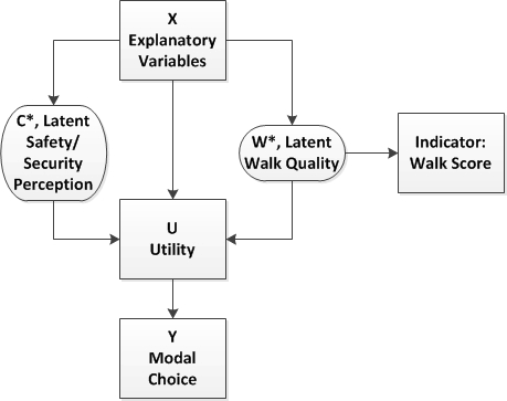
Figure 10. Illustration. Hybrid choice model with latent variables.
The case study presented in this chapter highlights and leverages new data sources that are publically available and ready to be integrated in tools and models at very low cost which would allow improving current models and improving the accuracy of predictions without costly survey work. Accordingly, multiple data sources are combined to capture network and non-network impacts on travel choice. This section provides a detailed description of the datasets that are used to estimate the mode choice model. Figure 11 illustrates the variety of information used for modeling.
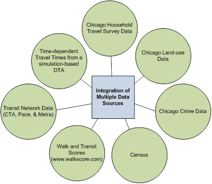
Figure 11. Illustration. Integration of multiple data sources.
Spatially Disaggregated Information About Walk Quality and Safety in Chicago, IL
Walk and Transit Scores
Walk Score™ is an increasingly popular measure of a location’s walkability.(101) Using the free walk score Application Programming Interface (API) and the longitude and latitude of Chicago Transit Authority (CTA) bus stops, each stop was assigned a walk score between 1 and 100 as defined by the Walk Score™ creators:
To compute a walk score, points are awarded based on the distance to amenities by categories, where amenities within 0.25 mi receive maximum points, and no points are awarded for amenities further than 1 mi.(102)
Similarly, a transit score is a measure of transit accessibility computed using General Transit Feed Specification data. As with the other transit network accessibility measures, since household travel information was available for a single point in each TAZ, the transit score for this particular point (not the exact location of a trip start or end), is not particularly meaningful. It was included for completeness, but not as significant as the developed measure of transit accessibility for estimating mode choice. The definition for transit score is as follows:
Crime Data
The Chicago Police Department’s crime dataset reflects reported incidents of crime (with the exception of murders where data exists for each victim) that occurred in Chicago, IL, from 2001 to the present. In order to protect the privacy of crime victims, addresses are shown at the block level only, and specific locations are not identified. Since crime rates vary by season and year, this analysis combines crime data from 2005–2008 to represent what may be travelers’ overall perceptions of crime in different areas. Crimes were categorized and aggregated for each origin and destination TAZ in the Chicago Metropolitan Agency for Planning (CMAP) household travel tracker survey (see figure 12). The crimes were categorized according to the Federal Bureau of Investigation’s crime classification codes (see table 3). Because it is anticipated that crime will be higher where there are more people, total TAZ crimes by category are divided by TAZ population to obtain a density as opposed to a count.
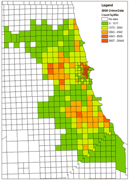
Figure 12. Illustration. Chicago, IL, crime count at the TAZ level in 2008.
Table 3. Crime categories tested in model.
| Category | Definition |
| Index | More serious offenses. Homicide first and second degree, criminal sexual assault, robbery, aggravated assault, aggravated battery, burglary, larceny, motor vehicle theft, and arson. |
| Non-index | Less serious offenses. Involuntary manslaughter, simple assault, simple battery, forgery and counterfeiting, fraud, embezzlement, stolen property, vandalism, weapons violation, prostitution, drug abuse, gambling, offenses against family, liquor license, disorderly conduct, and miscellaneous non-index offense. |
| Property | Burglary, larceny, motor vehicle theft, and arson. |
| Violent | Homicide first and second degree, criminal sexual assault, robbery, aggravated assault, and aggravated battery. |
| Aggravated assault | An unlawful attack by one person upon another wherein the offender displays a weapon in a threatening manner. Placing someone in reasonable apprehension of receiving a battery. |
| Aggravated battery | An unlawful attack by one person upon another wherein the offender uses a weapon or the victim suffers obvious severe or aggravated bodily injury involving apparent broken bones, loss of teeth, possible internal injury, severe laceration, or loss of consciousness. |
| Drug abuse | The violation of laws prohibiting the production, distribution, and/or use of certain controlled substances and the equipment or devices utilized in their preparation and/or use. |
| Index transit | Index crimes occurring in/on transit vehicles, stations, platforms, or facilities. |
Time-Dependent Travel Times
Data on the comparative travel times and travel costs of competing modes (CTA bus and rail and Metra rail) for each trip are obtained from network databases. Auto travel times are estimated based on time-dependent origin-destination travel times obtained from a simulation-based DTA model, Dynamic Network Assignment-Simulation Model for Advanced Roadway Telematics (DYNASMART).(102) When skimmed travel times were not available, mode-specific average speeds were used to estimate travel times. Table 4 shows the average speeds obtained from the reported travel times of the chosen alternatives in the survey data.
Table 4 . Mode-specific average speeds from Chicago, IL,
Household Travel Survey data.(103)
| Mode | Average Speed (mi/h) |
| Auto | 14.4 |
| Bus | 5.9 |
| CTA rail | 8.5 |
| Metra rail | 17.7 |
Chicago Household Travel Survey
The main source of data was the 2008 Travel Tracker Household Survey conducted in the northeastern Illinois region during 2007 and 2008 by CMAP.(104) Travel diary information with origin and destination information reported trips (figure 13) was collected from 14,390 households in the Chicago, IL, region, including some households in western Indiana and southern Wisconsin.
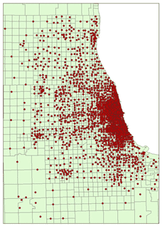
Figure 13. Illustration. Map of approximate locations of all origins and destinations
recorded in the CMAP Household Travel Survey data.
The dataset includes a total of 78,681 recorded trips with the four following trip purposes:
Travel costs for auto and CTA bus/train were estimated using figure 14 through figure 16 based on the Federal rates for privately own vehicle mileage reimbursement:
![]()
Figure 14. Equation. Auto cost estimation.
![]()
Figure 15. Equation. CTA bus/train cost estimation.
![]()
Figure 16. Equation. Metra train cost estimation.
Fares for Metra rail are estimated based on a distance-based zonal system, as shown in table 5.
Table 5 . Distance-based Metra fares.(105)
| Zone | Distance (mi) | Fare ($) |
| A | 0–5 | 1.95 |
| B | 5–10 | 2.14 |
| C | 10–15 | 3.05 |
| D | 15–20 | 3.45 |
| E | 20–25 | 3.91 |
| F | 25–30 | 4.32 |
| G | 30–35 | 4.68 |
| H | 35–40 | 5.14 |
| I | 40–45 | 5.55 |
| J | 45–50 | 6.00 |
| K | 50–55 | 6.41 |
| M | > 55 | 7.32 |
Chicago, IL, Land Use Data
Land uses were obtained from CMAP’s 2005 land use inventory. The inventory was created using digital aerial photography supplemented with data from numerous Government and private-sector sources. The land use data identify areas as small as 1 acre using a 49-category classification scheme. The following list presents main classes included in the database:
For this analysis, the list was reduced to five classes: residential, commercial, institutional, industrial, and other. In order to examine the effect of mixed use development on traveler behavior, several dummy variables at different spatial scales (with a radius of 0.25, 0.5, and 1 mi) were created for trip origin and trip destination, separately. These dummies were not significant in the model, and ultimately a measure of land use mix was most significant. Land use mix diversity index was estimated at different spatial scales (with radius of 0.25, 0.5, and 1 mi). The land use mix diversity index is computed as proposed by Bhat and Gossen and Rajamani et al. using figure 17 .(106,94)

Figure 17. Equation. Land use mix diversity index.
Where:
Res = The area of residential land.
Com = The area of commercial and services land.
Ind = The area of industrial land.
Ins = The area of institutional land.
O = The area of all other classes.
T = The total area around the desired location.
The mix diversity index is zero if land use is completely homogenous with only one class. The mix diversity index is equal to 1 if land use is fully mixed with equal proportion of all included land use classes.
Census Data
Census data include housing, population, and employment information at the smallest possible spatial aggregation (tract level). Population, housing, and employment densities were calculated for each trip origin and destination recorded in the Chicago Household Travel Survey data. Figure 18 shows a map of the population density in the Chicago, IL, metro region at the TAZ level.
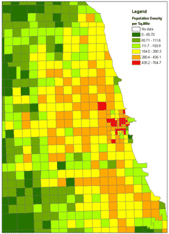
Figure 18. Illustration. Population density in the Chicago, IL, metro region at the TAZ
level from Census data.
Transit Network Data
Added to the land data are information from CTA, Pace (the premier suburban transit provider in Chicago’s suburbs), and Metra. The transit network in Chicago covers many suburbs and is strongly oriented toward the CBD.
For each trip origin and destination separately, several dummy variables at different spatial scales (with radius of 0.25, 0.5, 0.75, and 1 mi) were created to reflect the following transit accessibilities:
Ultimately, due to the precision of origins and destinations for each observation, these accessibilities were also reduced to a simple indicator of whether there was transit within a 0.25-mi radius of the origin or destination. This loss of resolution is due to insufficient observations of individuals over the course of a typical week and the aggregation of origins and destinations to a zonal centroid. Without knowing the precise origin and destination point of each traveler, it is difficult to determine exactly how accessible transit is for a given trip. Figure 19 through figure 22 provide the geo-coded location of the CTA bus stops, Pace bus stops, CTA train stops, and Metra train stops, respectively.
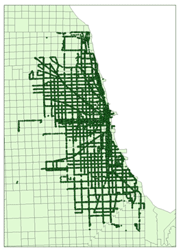
Figure 19. Illustration. Geo-coded locations of CTA bus stops.
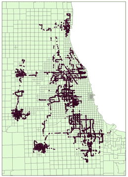
Figure 20. Illustration. Geo-coded locations of Pace bus stops.
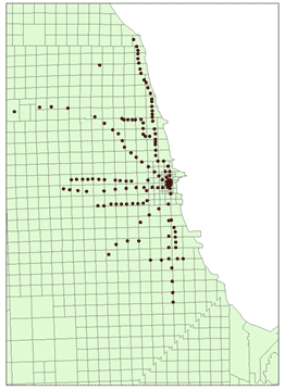
Figure 21. Illustration. Geo-coded locations of CTA train stops.
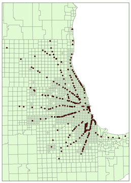
Figure 22. Illustration. Geo-coded locations of Metra train stops.
Mixed logit models were estimated to test combinations of variables until a satisfactory exploratory model was found. The final model is described in table 6. The most significant crime category influencing mode choice was drug use, though it was only significant in explaining urban transit mode choice, not suburban rail.
Travel time and travel cost divided by income had a negative impact on mode choice as expected. Since theory and common sense suggest that the importance of cost should decrease with income, cost was divided by the income. The values of time had to be adjusted to reflect the income units. As the travel costs are in dollars, travel time in minutes and income in dollars per year, the value of time spent in travel to the value of time spent working can be calculated by multiplying the ratio of the parameters by 12. That is, the estimated parameters, which are used to generate a distribution, from which the mean can be simulated. This gives a mean ratio of value of time spent in travel to value of time spent working of 0.23. This is in line with obtained values from other studies, which suggest a value of time in Chicago for traveling of around $10/h, which is smaller than the mean income.
The travel time index, a measure of congestion, is the ratio of reported travel time to free-flow travel time. The negative sign on this variable may indicate the self-selection of auto users versus choice transit users. Travelers are more likely to use transit for work trips and much more likely to use transit if the trips start and/or end in CBD due to the downtown-oriented transit systems.
The effects of land use diversity and density on urban transit use (i.e., CTA) corroborate the findings of Cervero.(56) Origin population and destination job densities increase transit use but tend to decrease suburban rail (Metra) use. This negative effect could be due to the relatively large catchment areas for suburban rail. The number of park and ride spaces was not a significant variable for either mode, which is probably due to the practice of parking on neighborhood streets to access transit. Similarly, origin land use mix is not a significant variable for predicting suburban rail, probably because of the nature of the suburban areas served. Land use mix was significant and positive at the destination end for both urban and suburban rail.
In exploring model specifications, it was found that crime types were highly correlated. Detailed factor analysis of crime and how it influences transit use is a topic left for further research. Incidences of reported drug abuse tend to decrease transit use, but this is only significant for urban transit. The lack of significance for urban rail may be due to the differences in nature of the stations or opportunities for crime between these mode types.
Table 6. Mixed logit mode choice model.
| Variable | Estimate | Standard Error | t-Value |
| Intercept | |||
| CTA | -3.350 | 0.268 | -12.518 |
| Metra | -6.440 | 0.434 | -14.854 |
| Dynamic travel time | -0.014 | 0.001 | -14.452 |
| Standard deviation of travel time | 0.031 | 0.012 | 8.213 |
| Travel Time Index | |||
| CTA | -0.091 | 0.012 | -7.447 |
| Metra | -0.086 | 0.021 | -4.094 |
| Cost/Income | -1.191 | 0.348 | -3.419 |
| Ratio of Vehicles to Household Members | |||
| CTA | -3.361 | 0.148 | -22.743 |
| Metra | -0.735 | 0.176 | -4.180 |
| Trip Purpose is Work | |||
| CTA | 1.149 | 0.094 | 12.196 |
| Metra | 1.570 | 0.178 | 8.831 |
| Start and/or end in CBD | |||
| CTA | 2.308 | 0.130 | 17.788 |
| Metra | 4.356 | 0.243 | 17.889 |
| Transit Accessibility of Destination | |||
| CTA | 0.544 | 0.134 | 4.062 |
| Metra | 0.104 | 0.173 | 0.597 |
| Walk Score of Origin | |||
| CTA | -0.007 | 0.004 | -1.983 |
| Metra | 0.007 | 0.005 | 1.539 |
| Walk Score of Destination | |||
| CTA | 0.011 | 0.003 | 3.608 |
| Metra | 0.016 | 0.006 | 2.915 |
| Origin End Population Density (1,000/1 mi) | |||
| CTA | 0.051 | 0.000 | 5.851 |
| Metra | -0.097 | 0.000 | -6.261 |
| Destination End Job Density (1,000/1 mi) | |||
| CTA | 0.080 | 0.000 | 5.490 |
| Metra | -0.029 | 0.000 | -1.030 |
| Origin Land Use Mix (0.25) | |||
| CTA | 1.713 | 0.306 | 5.604 |
| Metra | -0.741 | 0.453 | -1.635 |
| Destination Land Use Mix (0.25) | |||
| CTA | 0.842 | 0.307 | 2.743 |
| Metra | 1.484 | 0.602 | 2.467 |
| Drug Abuse Crimes/1,000 Population (0.25 mi) | |||
| CTA | -6.807 | 0.003 | -2.262 |
| Metra | -0.200 | 0.002 | -0.100 |
Based on the results presented in the table, the log likelihood is -2784.4, and the McFadden R2 value is 0.484.
The Household Travel Survey data used in this analysis were aggregated by zone, and origin and destination points were designated to protect the privacy of survey respondents. This kind of aggregation results in a loss of specificity, and measures such as land use diversity and transit accessibility are not exact for each individual.
Another limitation of the data and model is the inability to capture longer-term higher order decisions that may be influenced by policy. For instance, a number of attributes were not significant at the origin but were significant at the destination. This may reflect self-selection of respondents in that their origins were fixed whereas the destinations (at least for non-work trips) were somewhat more flexible. The opposite could be said for work trips: employees are not always able to select their work location. The selection of residential and work locations should be understood in the context of shorter-term decisions.
Recommended Next Steps and Research
There has been relatively little comprehensive cross-disciplinary exploration of the quality of life implications of travel. The physical activity afforded by walk trips—for whatever purpose—is of considerable interest to the public health community.(107,108) Research and implementation of environments that promote physical activity exist in Atlanta (e.g., strategies for metropolitan) and Seattle (e.g., land use, transportation, air quality, and health), and the recent panel studies of these travelers could be of great value for future research in non-network factors and active transportation. Crime is difficult to measure and even harder to predict, so the studies discussed here offer only snapshots of elements of the relationship between crime and transit mode choice. Capturing data on public health and safety in conjunction with travel behavior studies could illuminate these relationships. As in this study, such data may be combined from multiple sources, but the quality and level of capture of each data element cannot be overlooked. Open data may be the key to effectively integrating behavioral methods and concepts from psychology, sociology, geography, and transportation.
Such analyses require not only better measures of the walking environment and safety statistics, but also capturing trips by alternative modes. Passive data collection methods such as GPS and accelerometers on cell phones could be used to capture these trips without burdening the study subjects.(109) Longitudinal data collection is especially needed to capture self-selection and strategic behavior on the part of travelers, which influences the magnitude and significance of non-network effects at both origin and destination, and changing attitudes of travelers over time.
The case studies presented in chapters 5 through 8 represent advances in the state of the art and a significant step toward advancing the state of the practice in capturing user behavioral responses to operational and management interventions in assessment and simulation models. However, they are limited by the lack of sufficient data to calibrate all parts of the behavioral models. Conversely, the case study presented in this chapter highlights and leverages new data sources that are publically available and ready to be integrated in tools and models at very low cost which would allow improving current models as well as the accuracy of predictions without costly survey work.
Going beyond the immediate application presented in this chapter, the Internet has profoundly transformed activity engagement by creating virtual worlds or environments for activities, such as work and shopping, commonly pursued in the physical world. For travel behavior and time use analysts, virtual environments provide new opportunities for investigating decisions within a potentially experimental setting but also new opportunities to obtain rich data sources to integrate within models. Given the increasing engagement in online activities, such as social networking or games, understanding time use and travel decisions within these virtual environments may lead to an improved understanding of time use and travel in the physical environment. Individuals are increasingly engaging in virtual world activities, sometimes simultaneously or in conjunction with physical world activities.(110,111) Considering a set of activities that are engaged in the physical and a set in the virtual world, the set of activities that occur in both worlds can be conceptualized as the intersection of these two sets. As the opportunities for activity engagement in the virtual world continue to grow, a gradual eclipsing between these two worlds occurs.
Travel behavior and time use analysts have shed some light on this eclipsing by examining the role of information and communication technologies for work-related activities, from both a work management perspective and a travel/spatial location perspective. (See references 112–116.) For future research, such data from virtual worlds could be utilized and integrated further. Areas that come to mind include the following: