U.S. Department of Transportation
Federal Highway Administration
1200 New Jersey Avenue, SE
Washington, DC 20590
202-366-4000
Federal Highway Administration Research and Technology
Coordinating, Developing, and Delivering Highway Transportation Innovations
| REPORT |
| This report is an archived publication and may contain dated technical, contact, and link information |
|
| Publication Number: FHWA-HRT-13-097 Date: September 2014 |
Publication Number: FHWA-HRT-13-097 Date: September 2014 |
Simulate the Degree to Which Weather-Related Information Influences Travelers’ Pre-Trip Travel Decisions
Background
Weather events such as precipitation, fog, high winds, and extreme temperatures cause low visibility, slick pavement, reduced roadway capacity, and other hazardous conditions on roadways. The disruptive effect of inclement weather on traffic has staggering impact on safety. About 28 percent of all highway crashes and 19 percent of all fatalities involve weather-related adverse conditions. Additionally, adverse weather accounts for about 25 percent of delays on freeways due to reduced service capacity (often at the most critical of times) and greater risk of accident involvement. To mitigate the impacts of adverse weather on highway travel, the FHWA WRTM program has been involved in research, development, and deployment of WRTM strategies and tools. Dealing with adverse weather requires not only sensing traffic conditions, but also the ability to forecast weather in real time for operational purposes. Recognizing the importance of tying weather and traffic management together in areas exposed to extreme weather situations, such as hurricanes and floods, some TMCs, such as the Houston TranStar® TMC, co-locate the weather service personnel with the usual traffic management agencies (police, traffic operators, emergency medical services, etc.). The most ambitious initiative in this regard is the Clarus weather system, which intended to provide TMCs with accurate real-time weather information.(168–170) Weather information, along with roadway traffic information obtained from ITS sensors, enables promising opportunities to improve traffic operations and management under inclement weather.
To reduce the impacts of inclement weather events and prevent congestion before it occurs, weather-related advisory and control measures could be determined for predicted traffic conditions consistent with the forecast weather (i.e., anticipatory road weather information, which then can be used to inform travelers and influence their behavior). This calls for integrated WRTM and a traffic estimation and prediction system (TrEPS) together with an integrated demand model to estimate user behavior changes due to en-route and pre-trip road weather-related information. Because the dynamics of traffic systems are complex, many situations necessitate strategies that anticipate unfolding conditions instead of adopting a purely reactive approach.
In a previous FHWA project, a methodology for incorporating weather impacts in TrEPS was developed.(171,172) The project addressed supply and en-route demand aspects of the traffic response to adverse weather. The methodology was incorporated and tested in connection with the DYNASMART simulation-based DTA system, thereby providing a tool for modeling the effect of adverse weather on traffic system properties and performance and for supporting the analysis and design of traffic management strategies targeted at such conditions. The projects concluded that to be able to retain a similar level of service (LOS) as observed in clear weather conditions, en-route WRTM strategies need to be combined with ATDM strategies to reach a demand reduction between 15 and 20 percent.
The purpose of the current case study was to integrate demand models into weather responsive TrEPS to study and simulate behavior responses from travelers on different behavioral levels due to WRTM strategies in conjunction with ATDM strategies and policies to estimate and simulate traveler behavior responses due to pre-trip information and policy integration.
Simulate WRTM Strategies Integrated with Demand Models
TrEPS is an essential methodology to enable implementation and evaluation of traffic management, as it estimates and predicts network states. DYNASMART, developed largely under FHWA support, uses a simulation-based DTA approach for traffic estimation and prediction.(173,174) TrEPS must recognize the fact that origin-destination demand can only be reliably available if they are integrated with the corresponding demand models, estimating and predicting demand changes with underlying disaggregated behavioral models. Conversely, demand models will only be able to realistically reflect behavior if they incorporate dynamic and disaggregated LOS variables. Such disaggregated LOS variables are only available in the connection with a DTA approach. As a state-of-the-art TrEPS, DYNASMART combines advanced network algorithms and models en-route tripmaker behavior route choices in response to information in an assignment-simulation-based framework to provide estimates of network traffic conditions, predictions of network flow patterns in response to various en-route contemplated traffic control measures and information dissemination strategies, and anticipatory traveler and routing information to guide tripmakers in their travel.(175) In the previous FHWA project, the principal supply side and en-route demand side elements affected by adverse weather were systematically identified and modeled in the TrEPS framework (see figure 131).(171,172) The models and relations were calibrated using available observations of traffic and en-route user behavior in conjunction with prevailing weather events. The proposed weather-related features have been implemented in DYNASMART and demonstrated through successful application to a real world network, focusing on two aspects: assessing the impacts of adverse weather on transportation networks and evaluating effectiveness of en-route weather-related advisory/control strategies in alleviating traffic congestion due to adverse weather conditions. The procedures implemented immediately provide applicable tools that capture knowledge accumulated to date regarding weather effects on traffic. The application to a real-world network shows that the proposed model can be used to evaluate weather impacts on transportation networks and the effectiveness of weather-related VMSs and other strategies.
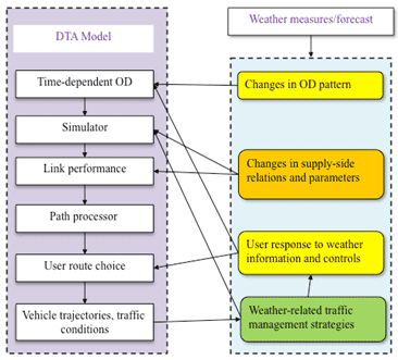
Figure 131. Illustration. Integrated DTA model with weather measures/forecast.(171)
Program Intervention: WRTM Strategies
Road weather information, such as en-route weather warning and route guidance, can be disseminated through radio, Internet, mobile devices, roadside VMS, etc. Pre-trip traveler information can be disseminated trough similar media channels and using social networking tools such as Twitter®.
Weather warning VMSs have been implemented in the field and are shown to be effective in decreasing the average speed as well as the variance in speed and hence helpful in increasing safety and reliability for the traveling public.(176,177) Weather VMSs also proved most effective when adverse weather and road conditions were not easy to detect. Weather advisory VMSs, in the form of slippery road condition sign and fog (low visibility) sign, have been implemented and tested in Europe. For example, in Finland, a slippery road condition sign, implemented in combination with a minimum headway sign, decreased the mean speed by 0.75 mi/h with the steady display and by 1.31 mi/h when the sign was flashing.(176) Hogema and van der Horst showed that the Dutch fog warning signs, implemented in conjunction with variable speed limits, decreased the mean speed in fog by 5 to 6 mi/h.(178) Conversely, Cooper and Sawyer found that the automatic fog-warning system on the A16 motorway in England reduced the mean vehicle speed by approximately 2 mi/h.(179) A comprehensive synthesis of recent developments and applications focusing on U.S. practice is presented in Developments in Weather Responsive Traffic Management Strategies.(180)
Weather-related pre-trip information has not been studied in depth so far, but pre-trip traveler information in general as part of ATIS strategies has been studied. It has been found that traveler information influences route, departure-time, and mode choice. Abdel-Aty et al. studied route changes in Los Angeles, CA.(181) Only a small share of the respondents (15 percent) reported using more than one route on their commute. Of that 15 percent, 34 percent said they changed routes after actually seeing traffic conditions. Higher incomes and education levels predicted more route changes, perhaps reflecting schedule flexibility and arrival times expectations for such workers. Mahmassani et al. performed a survey of commuters in Austin, TX, to study information dissemination and traveler behavior. Information in the form of radio traffic reports appeared to have a strong impact in that regular listeners to traffic were more likely to switch their behavior with new information.(40)
Mahmassani and Changstudied an adjustment and experience-based model of perceived travel time for departure time choice.(58) Under the myopic adjustment rule, the perceived travel time is only a function of the latest day’s outcome. In laboratory experiments conducted to study the effectiveness of different information strategies on user responses to information, Srinivasan and Mahmassani found that route switching model specifications, which predict whether a user will switch paths in a given time interval, consistently outperformed models that view the process as a new choice at every opportunity.(182) The authors designed an experiment whereby virtual commuters were given trip times on three facilities (at decision locations), information about congestion on the facilities, a message alerting the driver when they are stuck in a queue, and post-trip feedback consisting of departure time, arrival time, and trip time on the chosen path. Their empirical findings suggest that an individual’s negative experience with ATIS information has mixed effects on inertia, but congestion and information quality tend to reduce inertia. Drivers who experience lower switching costs and increased trip time savings tend to comply with information. In the sequential treatment, past negative experience relative to preferred arrival time seemed to increase the likelihood of compliance. Inaccurate information decreased drivers’ compliance propensity.
Beyond these dimensions, only a couple of studies have addressed destination adjustment in response to information for discretionary (shopping) travel.(44)
Managing demand in this case study encompasses providing travelers with information aimed at creating a shift in their departure times, a mode shift, or a trip cancelation so that the total travel demand during the peak periods can be reduced. The objective was how much demand should be reduced under different weather conditions in order to maintain a certain level of network performance and how this demand reduction could be achieved. It is critical for the traffic operators to provide reliable information to maintain credibility with roadway users. It is also important to try to minimize the potential economic losses by setting the target demand to its necessary level. Attempting to reduce demand beyond this level might cause significant financial loss to the local business and community. As such, the goal of using TrEPS is to provide traffic operators with the information on the optimal level of demand that can improve the network performance but not negatively affect the productivity under given weather conditions, information on which strategies the appropriate demand reduction can be achieved.
Behavioral Dimensions: Route Choice, Departure Timing, Mode Choice, and Trip Cancellation
The previous discussion of prior work reveals that efforts to devise WRTM systems have remained limited to a few countries and locales, although recognition of the need for such intervention continues to increase. Furthermore, the incorporation of demand models into existing tools responsive to WRTM are missing so far and constitute an important link for the usefulness of WRTM applications in practice. Whereas the studies so far highlighted the en-route information influence through VMS on route choice decisions, this case study focuses on simulated behavior responses based on pre-trip information. Since WRTM strategies target short- to medium-term decisions due to the limited time frame of weather forecasts, the immediate behavioral dimensions that can be influenced with pre-trip and en-route weather-related traffic information are route choice departure time choice, mode choice, and trip cancellation. To capture the behavior in a responsive way, spatially and temporally disaggregated individual-based models were used in conjunction with the mesoscopic DTA simulation.
The advantages of using disaggregated individual demand models on WRTM strategies can be grouped into the following categories:
The modeled behavior choices for households and individuals were organized sequentially on the basis of the time frame over which they might take place. As a result, longer-term decisions were modeled first, followed by medium- and then short-term decisions. Thus, each of the models imposes certain restrictions on the sub-sequential decisions on a shorter time horizon. This conceptual framework was used for integrating the demand model with the network assignment procedure to evaluate WRTM strategies and is further explained in the following section.
Framework for Evaluation
When analyzing WRTM strategies in terms of their impacts on the flows in the network, one has to consider that demand, which is used as an input for the network assignment, is affected by the changes in the generalized cost function values produced in the traffic assignment. Thus, the integration of transport supply and demand models is important, as the demand and supply models are each formulated to use forecast outputs from the other model.
This section discusses the feedbacks between the demand and supply models as well as what level of intersection for the feedback loops is appropriate to study and analyze WRTM strategies so that the level of service input to the demand models is the same as the output from the supply models and the demand input to supply models is the same as that output from the demand models.
The integration of demand models and the network assignment to evaluate WRTM strategies has several parts. First, a base travel demand with calibrated travel costs and skims was generated, which was then used to update the travel times and cost skims by solving for the multi-criterion dynamic user equilibrium. Second, bad weather scenarios were introduced on the network level with weather adjustment factors (WAFs). The changed supply on the network level was then used to update the travel time and cost skims by solving again for the multi-criterion dynamic user equilibrium. Third, the generated disaggregated user time and cost skims were fed back to the individual disaggregated demand model, where the travel time and cost skims propagated through the sequence of interrelated choices and affect particularly all the short- and medium-term traveler decisions shown in figure 132. This includes direct impacts of weather on mode and departure time choice (as well as location choice, which is not shown here) through generalized cost functions included in the utility expressions for each choice alternative.
However, in the medium to long term, bad weather scenarios in places where they occur frequently can also indirectly affect further user decisions, such as activity pattern changes and accessibility, as well as even longer-term choices of home, workplace, and school location (not illustrated).
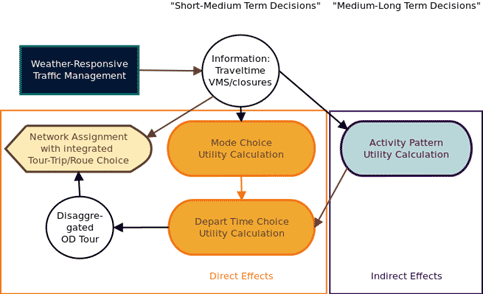
Figure 132. Illustration. WRTM modeling framework.
The supply side used in this case study was calibrated based on a previous study and is discussed in more detail in Mahmassani et al.(171,172) Supply-side parameters that are expected to be affected by the weather condition are identified in table 22.
Table 22. Supply-side properties related with weather impact in DYNASMART.(171)
| Category | mi/h | Parameter Description |
| Traffic flow model1 | 1 | Speed-intercept (mi/h)1 |
| 2 | Minimal speed (mi/h) | |
| 3 | Density break point (pcpmpl)1 | |
| 4 | Jam density (pcpmpl) | |
| 5 | Shape term alpha | |
| Link performance | 6 | Maximum service flow rate (pcphpl or vphpl) |
| 7 | Saturation flow rate (vphpl) | |
| 8 | Posted speed limit adjustment margin (mi/h) | |
| Left-turn capacity | 9 | Effective green-to-cycle length (g/c) ratio |
| Two-way stop sign capacity | 10 | Saturation flow rate for left-turn vehicles (vphpl) |
| 11 | Saturation flow rate for through vehicles (vphpl) | |
| 12 | Saturation flow rate for right-turn vehicles (vphpl) | |
| Four-way stop sign capacity | 13 | Discharge rate for left-turn vehicles( vphpl) |
| 14 | Discharge rate for through vehicles (vphpl) | |
| 15 | Discharge rate for right-turn vehicles (vphpl) | |
| Yield sign capacity | 16 | Saturation flow rate for left-turn vehicles (vphpl) |
| 17 | Saturation flow rate for through vehicles (vphpl) | |
| 18 | Saturation flow rate for right-turn vehicles (vphpl) | |
| 1Only available in dual-regime model. pcpmpl = Passenger cars per mile per lane, pcphpl = Passenger cars per hour per lane, and vphpl = Vehicles per hour per lane. |
||
The inclement weather impact on each of these parameters is represented by a corresponding WAF as follows:
![]()
Figure 133. Equation. WAF.
Where:
fiWeather Event = The value of parameter i under a certain weather event.
fiNormal = The value of parameter i under the normal condition.
Fi = The WAF for parameter i.(172)
Behavioral Models
Utility-based econometric models have their roots in economic consumer choice theory. These model the individual’s activity and travel decisions. In addition to discrete choice alternatives, these models can be enriched by other utility-based models such as hazard models to represent time durations. Overall, the set of economic equations provide the structure to model the relationship between the traveler’s characteristics, the network characteristics, and the environment’s characteristics, which describe the place to perform activities and also any further restrictions on the traveler's behavior.
The utility-based choice models used to represent the mode and departure time choices follow the concept of an overarching daily activity travel pattern proposed by Bowman and Ben-Akiva.(183) These models are based on an underlying system of logit models in a particular hierarchy. Detailed model forms and specifications are presented later in this chapter.
Data Available and Used in Case Study
Urban Network and Associated Weather Conditions
The network used in this case study included the Chicago, IL, downtown area along the Kennedy and Edens Expressways. The network is bounded on the east by Lake Michigan and on the west by Cicero Avenue and Harlem Avenue. Roosevelt Road and Lake Avenue bound the sub-network from the south and north, respectively. The network description is illustrated in figure 134. The network description is as follows:
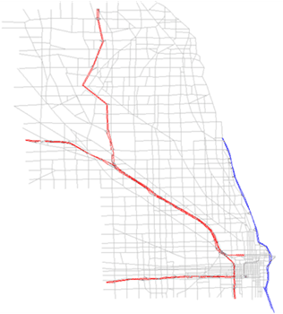
Figure 134. Illustration. Network configuration and description for Chicago, IL, network.
Weather Data
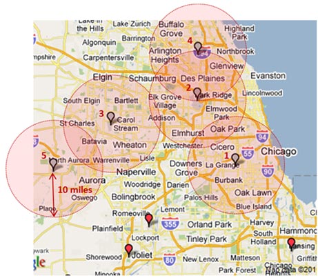
Weather data are available from two sources; the Automated Surface Observing System (ASOS) stations located at airports and the roadside environmental sensor stations (ESSs) available on the Clarus Web site. As the historical weather data from ESS have a time resolution of 20 min and are only available from 2009 to the present, ASOS data with 5-min resolution were used in conjunction with traffic detector data collected and aggregated over a 5-min interval. ASOS 5-min weather data are available on the National Oceanic and Atmospheric Administration’s National Climatic Data Center Web site. The spatial distribution of ASOS stations used in this case study is shown in figure 135, and their location and further information are listed in table 23.
©Google Maps® 2012
Figure 135. Illustration. Chicago, IL, study area and adjacent ASOS stations.(184)
Table 23. Airports with ASOS stations and available time periods for data.
| No. | Airport | Location | ICAO Airport Code | ASOS Data |
| 1 | Midway International Airport | Chicago, IL | KMDW | 2005–Present |
| 2 | O’Hare International Airport | Chicago, IL | KORD | 2000–Present |
| 3 | Dupage County Airport | Dupage, IL | KDPA | 2005–Present |
| 4 | Chicago Executive Airport | Cook, IL | KPWK | 2005–Present |
| 5 | Aurora Municipal Airport | Kane, IL | KARR | 2005–Present |
| ICAO = International Civil Aviation Organization. | ||||
Traffic Data
In conjunction with the weather data described in the previous section, traffic data for supply side parameter calibration and aggregated analysis of demand data was obtained from loop detectors installed on freeway lanes. Historical data with the 5-min aggregation interval were used, and the time periods for the data varied with the study site over the 2005–2011 period.
In selecting detector locations and collecting the data, the following criteria were mainly considered:
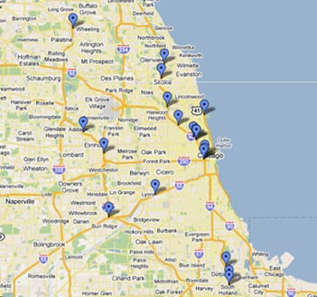
Note that the process for removing the effect of external events is highly dependent on the availability of other event data. In case where there is difficulty obtaining detailed data for incidents, work zones, and special events, one could focus on traffic data and clean outliers in the dataset only. Since average measures are extracted over a longer period of time (i.e., at least 1 year), the influence of other external events on traffic parameters is expected to be small. The selected loop detector locations are illustrated in figure 136.
For the Chicago, IL, network, traffic data were obtained from the Illinois Department of Transportation; 5-min aggregated data from 2009 were used. Figure 136 shows a map of the selected detector locations in Chicago, IL. At each location, traffic data from northbound or southbound directions were obtained. There was no HOV lane at any of the selected locations.
©Google Maps® 2012
Figure 136. Illustration. Selected detector locations in Chicago, IL.(185)
Behavioral Model Data
This section presents details of data preparation and model estimation for the individual behavioral models (mode choice and departure time choice).
Mode Choice:
The main source of data used to develop the mode choice and departure choice models in this study was the Chicago Household Travel Survey and National Transit Database (NTD), which were used to estimate travel times for the non-chosen modes (public transit in this case study).(186,187) Table 24 shows the average speeds obtained from the reported travel times of the chosen alternatives in the travel survey data.
Table 24 shows mode-specific average speeds obtained from the NTD for CTA, Pace, and Metra in 2011. The average speeds were calculated by dividing the annual vehicle revenue miles by the annual vehicle revenue hours for each mode. The average speeds obtained in the NTD are higher relative to the reported average speeds from the Chicago Household Travel Survey. Although the NTD speeds seem to be more realistic, the average speeds from the Chicago Household Travel Survey represent experienced travel time by transit users, perhaps including waiting time and travel time in all the segments of a transit trip (e.g., walking to/from transit stop). Therefore, for the purpose of this study, an average speed of 14.4 mi/h was used for the transit mode, and an average speed of 17.7 mi/h was used for the park & ride mode.
Table 24. Mode-specific average speeds from the 2011 NTD.
| Mode | Average Speed (mi/h) |
| CTA bus | 9.3 |
| Pace bus | 13.9 |
| CTA rail | 18.4 |
| Metra rail | 30.7 |
Travel costs for auto and transit are estimated using the following expressions:
![]()
Figure 137. Equation. Auto travel cost estimation.
![]()
Figure 138. Equation. Transit travel cost estimation.
Since the number of transfers was unknown, three different assumptions were made to estimate transit cost. First, it was assumed that all the transit trips were made with no transfers. Thus, transit cost for all the origins and destinations were fixed and equal to $2.25. The second assumption was that those trips that started and ended at non-CBD zones included one transfer, and the rest of the trips included no transfers. The third assumption was that those trips that started or ended outside Chicago’s boundary had an average transit cost of $4.50, while the rest of the trips with transit cost $2.50. Results of the mode choice model, which are described in the next section, suggest that assumption two provides more realistic values of time.
For the park & ride mode, the following equation was used to estimate travel cost (including transit fare and parking):
![]()
Figure 139. Equation. Park & ride travel cost estimation.
Departure Time Choice
For the departure time choice model, the initial demand as sliced into 0.5-h bins, and the dynamic travel times for the clear weather scenario and snow weather scenario were used to infer travel times.
If for the specific disaggregated origin-destination pair, based on network nodes (1,5782 combinations in the Chicago network), individual trips fall within the departure time bin, the average observed travel time for this origin-destination and half hour bin was used. If there were no observations from the DTA for a specific origin-destination and time bin were available, the free flow travel time was used.
It is assumed that the preferred arrival time for each individual was the arrival time under clear weather condition and the too late or too early arrival times under the snow weather conditions were then inferred based on the new travel times for each departure time bin.
Model Development and Calibration
Mode Choice
The empirical analysis of mode choice in this study applies the discrete choice modeling framework developed by Domencich and McFadden and Ben-Akiva and Lerman.(188,189) The model is segmented by trips from and to the CBD and trips occurring outside of the CBD. This market segmentation was applied, as the transit system in Chicago focused on commuting trips to and from the CBD. Transit shares for trips with origin and destination outside of the CBD had a very low share of 3.25 percent, where the shares for trips with origin or destination in the CBD were 44.73 percent. In addition, there are several park & ride locations that connect people in the Chicago suburbs to the commuter rail system, which is included as a separate mode in the mode choice model for CBD trips.
To realistically capture the substitution patterns between the different modes available, it is essential to consider the similarities between park & ride options and public transit option alone, as these two modes share unobserved attributes among each other, which violates the independence of irrelevant alternatives property of the multinomial logit model. To capture the similarity of park & ride trips and transit trips, a nested multinomial logit model was estimated for trips from and to the CBD and for trips outside the CBD a standard logit model is estimated with only the two alternatives auto and transit. The two models are described in table 25 and table 26.
Table 25 and table 26 show the parameter estimates for the nested logit model for the Chicago metropolitan area trips from and to the CBD and the parameter estimates for the logit model for the Chicago metropolitan area trips outside of the CBD, respectively.
Table 25. Nested logit model estimation results for trips from and to the CBD.
| Variables | Estimate | Standard Error | t-Value | p-value |
| Travel time | -0.01 | 0.00 | -12.00 | 0.00 |
| Cost | -0.07 | 0.01 | -10.97 | 0.00 |
| Park & ride intercept | -0.71 | 0.12 | -6.10 | 0.00 |
| Transit intercept | -0.07 | 0.06 | -1.17 | 0.24 |
| Park & ride departure time after 7 a.m. | -0.96 | 0.09 | -10.99 | 0.00 |
| Transit departure time after 7 a.m. | -0.55 | 0.06 | -9.16 | 0.00 |
| 0.70 | 0.06 | 12.47 | 0.00 | |
| Correlation | 0.51 | 0.10 | -5.29* | 0.00 |
| *Denotes that this t-value compares the difference betweennthis parameter estimate and a value of 1.0. | ||||
Based on this information, the likelihood at convergence is -17,965.64, and the value of time is 8.35, which is calculated as the ratio of the parameter for time over the parameter for cost. It is comparable to value of time obtained for Chicago in other studies. The value of time is on average slightly higher for trips to and from the CBD compared to trips outside of the CBD.
Table 26. Logit model estimation results for trips outside of the CBD.
| Variables | Estimate | Standard Error | t-Value | p-value |
| Travel time | -0.01 | 0.00 | -9.26 | 0.00 |
| Cost | -0.09 | 0.02 | -4.30 | 0.00 |
| Transit intercept | -2.16 | 0.16 | -13.15 | 0.00 |
| Transit departure time after 7 a.m. | -0.77 | 0.16 | -4.68 | 0.00 |
Based on this information, the likelihood at convergence is -2,748.41, and the value of time is 6.31.
Figure 140 and figure 141 showcase the nesting structure for the nested logit and logit models, respectively. The parameter estimates are consistent for both models. All estimates are as expected and highly significant. The nesting coefficient shows a medium correlation of park & ride with transit and is highly significant different from 0 and 1, where 0 would indicate perfect correlation and 1 no correlation. The transit and park & ride intercepts show the average attractiveness of each alternative compared to auto for all unobserved factors. In both models, the auto is the relative preferred mode of choice given all observed attributes being the same. Public transit options are rather used during rush hour period compared to off peak periods.
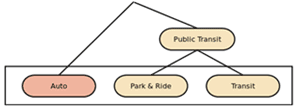
Figure 140. Illustration. Nested and non-nested mode choice model structure—structure for trips to and from the CBD
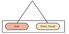
Figure 141. Illustration. Nested and non-nested mode choice model structure—structure for trips outside the CBD.
In the nested logit model framework, the utility of each alternative j to an individual i can be represented as follows:
![]()
Figure 142. Equation. Random utility model.
Where:
Uij = Utility of alternative j for individual i.
xij = Exogenous characteristics of individual i and alternative j.
b = Set of parameters.
eij = Error term distributed Gumbel with mode 0 and scale 1.
For the nested case, the utility for park & ride and transit can be rewritten with a shared error component as follows:
![]()
Figure 143. Equation. Utility of park & ride and transit.
Where:
UP&R = Utility of park & ride.
VP&R = Vector of park & ride.
ePT = Shared component.
eP&R=Error of park & ride.
UTransit = Utility of transit.
VTransit = Vector of transit.
eTransit = Error of transit.
The unobserved component of park & ride and transit are divided into two components. The distinct error components for park & ride and transit are represented by independent and identically distributed Gumbel random variables with variance parameter ![]() PT. The shared component, ePT, is distributed such that the sum of both distributions is Gumbel (0,1), as shown in the following equation.
PT. The shared component, ePT, is distributed such that the sum of both distributions is Gumbel (0,1), as shown in the following equation.
![]()
Figure 144. Equation. Distribution of nested logit error terms.
Where G(a,b) = The Gumbel distribution with mode a and scale b.
The problem can then be described as if there are two levels of choice: a marginal choice among auto and public transit and a conditional choice between park & ride and transit if public transit is chosen. Since eP&R and eTransit are independent and identically distributed Gumbel (0,![]() PT), where
PT), where ![]() PT is the scale of the Gumbel distribution for the transit error term, the condition choice becomes the following:
PT is the scale of the Gumbel distribution for the transit error term, the condition choice becomes the following:

Figure 145. Equation. Conditional choice probability (nested logit).
Where:
i= The set of all individuals.
j = The set of all alternatives.
![]() PT = scale of the Gumbel distribution for the transit error term.
PT = scale of the Gumbel distribution for the transit error term.
The marginal choice probability between auto and public transit is given by the following:
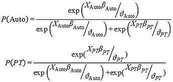
Figure 146. Equation. Marginal choice probabilities (nested logit).
The parameters in the nested logit probability formulation in figure 146 are estimated by maximizing the following log likelihood function:

Figure 147. Equation. Log-likelihood function (nested logit).
Where:
I = The set of all individuals.
yij = Choice indicator for alternative j and individual i, as defined in figure 148 .
P&R = Park & ride.
PT = Public transit.
![]()
Figure 148. Equation. Choice indicator function.
In the case of non-CBD trips, the usual multinomial logit modeling framework is used, where the probability of choosing between auto and transit is given by the following:

Figure 149. Equation. Choice probability.
Where P(j) is the probability of decisionmaker i choosing mode j.
Departure Time Choice
For the departure time choice model, the discrete-choice modeling framework developed by Domencich and McFadden and Ben-Akiva and Lerman is used.(188,189) Since there are no data available to specifically estimate the departure time choice coefficients, the model is calibrated using coefficient estimates from the model developed by Noland and Small and recalibrating the alternative specific constants to match the departure time choices observed in Chicago.(190)
A cost function is postulated with a particular preferred arrival time, which empirically is taken to be the arrival time under clear weather condition. This scheduling cost function, CS is calculated as follows:
![]()
Figure 150. Equation. Scheduling cost function.
Where:
Const. = Alternative specific constant for each 30-min departure time bin.
T = Free-flow travel time plus the extra travel time due to recurrent congestion which we assume the commuter expects will occur daily during clear weather.
TW = Added time due to non-recurrent (or unpredictable) congestion due to incident-related delays, which is the difference between the dynamic simulated travel time during bad weather condition and T.(191)
SDE = Schedule delay early.
SDL = Schedule delay late.
β1, β2, and β3 = Costs per minute of travel time, arriving early, and arriving late, respectively.
As the expected travel time for the clear weather condition is T, SDE and SDL are zero in the clear weather condition since no delays are expected. SDE and SDL for bad weather conditions are defined as follows:
![]()
Figure 151. Equation. Definition of schedule delay early and late.
Table 27 shows the parameter estimates for the departure time choice model.
Table 27. Departure time choice model parameter estimates.
| Variables | Estimate | Standard Error | t-Value | Pr(> |t|) | Significance Level |
| Travel time | -0.098 | — | — | — | — |
| SDE | -0.097 | — | — | — | — |
| SDL | -0.281 | — | — | — | — |
| Alternative Specific Variables | |||||
| 5:00–5:30 a.m. | Base category | ||||
| 5:31–6:00 a.m. | 1.406 | 0.23 | 11.62 | 0.00 | 0 |
| 6:01–6:30 a.m. | 3.460 | 0.56 | 8.35 | 0.00 | 0 |
| 6:31–7:00 a.m. | 4.939 | 0.92 | 6.45 | 0.00 | 0 |
| 7:01–7:30 a.m. | 7.273 | 1.02 | 9.23 | 0.00 | 0 |
| 7:31–8:00 a.m. | 9.506 | 1.23 | 12.23 | 0.00 | 0 |
| 8:01–8:30 a.m. | 11.689 | 2.56 | 7.32 | 0.00 | 0 |
| 8:30–9:00 a.m. | 13.698 | 2.34 | 13.11 | 0.00 | 0 |
| 9:01–9:30 a.m. | 15.382 | 2.86 | 14.23 | 0.00 | 0 |
| 9:31–10:00 a.m. | 17.123 | 3.21 | 9.10 | 0.00 | 0 |
| 10:01–10:30 a.m. | 16.060 | 3.51 | 8.11 | 0.00 | 0 |
| 10:31–11:00 a.m. | 13.110 | 2.32 | 8.32 | 0.00 | 0 |
| — Indicates where data are not applicable since these parameters were not estimated in this model. | |||||
Based on the information in the table, the likelihood at convergence is -52,621.3.
Natural Reduction
For the base scenario with bad weather, the amount of natural reduction in demand must be determined, as several studies have found that traffic volumes decline during winter storms.(192–194) This natural demand reduction without demand management strategies may be due to several reasons, including trip cancelation, teleworking, mode shifts, and departure time shifts. Hanbalifound demand reductions ranging from 7 to 56 percent during snow fall depending on time of day, day of the week, and roadway type as well as the strength of snowfall.(194)
For the Chicago, IL, case, the average traffic volumes for a moderate snow day and a clear weather day from several detectors on freeways (see figure 136) are compared to find an aggregated natural demand reduction to apply to the base weather scenario. The resulting difference in traffic is illustrated in figure 152. Overall, the observed reduction in traffic is 8.95 percent. Due to a lack of additional data sources (e.g., daily transit counts, detector data on peripheral roads, or Travel Household Survey data for bad and good weather days), it is unclear if a decrease in traffic volume is due to route choice, mode choices, departure time choice, or trip cancellation. However, the analysis of ICM case study suggests that the traffic reduction is mostly due to trip cancellation, as no mode shifts were observed, and the reductions were observed during non-peak hours when the infrastructure was not at capacity.
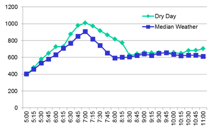
Figure 152. Graph. Traffic detector volumes on clear weather days and a median snow day in Chicago, IL.
Policy Intervention: Weather-Related Delay of Schools
A weather-related cancellation or delay of an institution, operation, or event as a result of inclement weather is common in many parts of the world, as well as in warmer parts of the United States, which are less likely to handle snow. Among institutions, schools are likely to close or delay when snow impairs travel. This is mostly due to concern about safety in order to keep those traveling to the location of the schools in an effort to prevent accidents.
Many countries and smaller jurisdictions have mandates for a minimum number of school days in a year. In order to meet these requirements, many public school systems and private schools that can expect to be closed at times during the year by inclement weather will often build a few extra days into their calendar for snow closures. Instead of cancelling an entire school day, some schools may delay opening by 1 or 2 h or announce a particular opening time. This can be advantageous in places where schools are not charged a snow day by delaying their opening. This is particularly common during lighter snowfalls in areas accustomed to moderate winter snowfall, such as the New York metropolitan area and adjacent southern New England; Washington, DC; Philadelphia, PA; and Baltimore, MD. In Chicago, there is no such policy in place. In order to prevent accidents as well as other problems that may result from travel in inclement weather, such a policy could be suggested and implemented on certain days in, especially as providing information to parents is simple and affordable through Internet media outlets.
In the event of snow, schools could delay opening by 1 or 2 h and extend the day for the time missed in the morning. Such a policy could have a significant effect since school-related trips have a very narrow departure time distribution during the peak hour. In Chicago, during the morning peak between 5 and 10 a.m., school-related trips constitute 8.9 percent of the traffic volume, and its departure time distribution is much narrower than work trips in the same time period. Figure 153 shows the distribution of work departure time and school trip departure time for autos. By shifting the school related trips by 1 h, the departure time distribution could be flattened and expanded toward later hours, which is especially interesting, as departure time interventions, such as earlier dissemination of information, shifts departure times toward earlier hours.
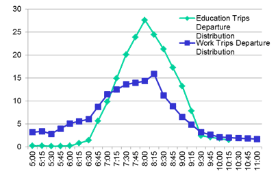
Figure 153. Graph. Morning peak departure time distribution for school trips and work trips
Sensitivity Analysis Using Simulation for Different Scenarios
Experiment Design—Weather Scenario:
For the weather scenario, a median snow day on February 22, 2011, in Chicago, IL, was chosen. The entire simulation horizon was 8 h, where vehicles were generated and loaded onto the network during the first 6 h based on the origin-destination matrix, which represents the traffic demand between 5 and 11 a.m. For the remaining 2 h, vehicles were simulated so that the generated vehicles reached their destinations.
Experimental Design—Demand Scenarios:
A total of 12 demand scenarios were prepared: one for the benchmark case, which was 100 percent of the demand under the normal weather condition (i.e., no snow); and the other 11 scenarios with different demand levels under snow condition. For the generation of the 11 scenarios, researchers started with the full demand (100 percent) and reduced the total demand with different demand management strategies as shown in table 28.
Table 28. Demand scenario overview and description.
| Scenario Number | Scenario Name | Demand Input | Description |
| 1 | Base— normal weather | Normal weather and normal traffic | Calibrated base scenario, which builds the basis for the subsequent scenarios |
| 2 | Base—weather | Moderate snow weather and normal traffic | Scenario to estimate the weather impact on the network LOS |
| 3 | Moderate weather—natural | Moderate weather, natural mode choice, and natural departure time spread | Scenario to estimate the LOS based on the natural reduction in trips and spread out of the peak hour |
| 4 | Moderate weather—natural and demand management | Moderate weather, natural mode choice, natural departure time spread, and VMS | Scenario to estimate the LOS based on the natural reduction in trips and spread out of the peak hour |
| 4.1.1 and 4.1.2 | Mode choice | 50 and 100 percent information | Scenario to estimate the LOS based on the natural reduction in trips and mode choice |
| 4.2.1 and 4.2.2 | Departure time choice | 50 and 100 percent information | Scenario to estimate the LOS based on the natural reduction in trips and departure time choice |
| 5 | Policy | Educational trips 1 h later | Scenario to estimate the LOS based on the natural reduction in trips and school opening delay of 1 h |
| 6 | Moderate weather—demand management and policy | Moderate weather, natural reduction, mode choice, departure time choice, and policy intervention | Scenario to reach the same LOS based on the natural reduction in trips and spread out of the peak hour, plus the on-route trip changes based on VMS, plus pre-trip changes based on earlier dissemination of weather information |
| 6.1 | 4.1.1, 4.2.1, and 5 | ||
| 6.2 | 4.1.2, 4.2.2, and 5 | ||
| Note: Blank cells indicate not applicable. | |||
DYNASMART Simulation
Analysis of the Results:
The following network performance measures are defined to illustrate network-level traffic conditions under different weather and demand scenarios:
![]()
Figure 154. Equation. Accumulated percentage of out vehicles.
Where:
OutVehicle = Accumulated number of vehicles arriving their destinations from time 0 till time t in each scenario.
TotalVehicle =Accumulated total number of vehicles loaded onto the network from time 0 till time t in each scenario.
![]()
Figure 155. Equation. Percentage change in average travel time.
Where:
Avg(TTimeBase) = Average travel time for full demand in the base case without weather feature.
Avg(TTime) = Average travel for each weather scenario.
![]()
Figure 156. Equation. Percentage change in average stop time.
Where:
Avg (STime) = Average stop time for k percent of full demand in weather scenario i.
Avg (STimeBase) = Average stop time for full demand in the base case without weather feature.
Scenarios 1 and 2:
Scenarios 1 and 2 are each used to establish a benchmark case to which the different other scenarios are compared. The first benchmark case, scenario 1, simulates traffic under clear weather condition with 100 percent demand. This scenario is used as the base scenario as described in figure 154 and figure 155. Scenario 1 is also used to establish a desired level of service which the different scenarios try to reach in order to maintain the same level of network performance as under clear weather condition.
Scenario 2 is used to establish the worst-case scenario under median snow condition with 100 percent demand and no management strategy, as well as no natural reduction. This scenario can be used to establish measures of improvement for the rest of the scenarios but also as an illustration of the impact of a median snow day on the network performance.
Figure 157 and figure 158 present the network density level using color coding where red = congested and green = uncongested for scenarios 1 and 2. In the figures, the time point for the current condition is set to 9:30 a.m. By comparing the two figures, it is clear that the network under clear weather is less congested than under median snow weather. Under snow weather condition, congested links (red) are more often observed and generally more widely spread in the network.
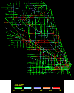
Figure 157. Illustration. Simulated network density for scenarios 1 and 2 with 100 percent demand—clear weather condition.
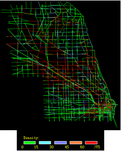
Figure 158. Illustration. Simulated network density for scenarios 1 and 2 with 100 percent demand—median snow day.
Figure 159 through figure 162 show a link-specific speed and flow distribution over the simulation time from 5 to 11 a.m. The selected link is the Kennedy Expressway between Pulaski Road and North Cicero Avenue westbound.
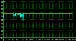
Figure 159. Illustration. Simulated link speed distribution for scenarios 1 and 2 for the Kennedy Expressway between Pulaski Road and North Cicero Avenue westbound—clear weather condition.
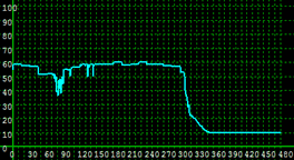
Figure 160. Illustration. Simulated link speed distribution for scenarios 1 and 2 for the Kennedy Expressway between Pulaski Road and North Cicero Avenue westbound—median snow day.
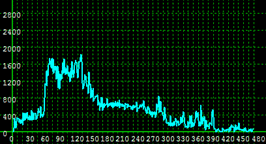
Figure 161. Illustration. Traffic volume distribution for scenarios 1 and 2 for the Kennedy Expressway between Pulaski Road and North Cicero Avenue westbound—clear weather condition.

Figure 162. Illustration. Traffic volume distribution for scenarios 1 and 2 for the Kennedy Expressway between Pulaski Road and North Cicero Avenue westbound—median snow day.
Comparing figure 159 and figure 160 shows the impact of the weather condition drastically, as the speed on the link breaks down at around 10 a.m. in the morning, which can also be seen when comparing the traffic volumes of these two links. The average travel time increases from scenario 1 to scenario 2 from 30.2 to 38.6 min, which is an average increase of 27.81 percent. Considering a value of time in Chicago of around $8/h and a total demand of ~800,000 travelers, the additional travel time due to bad weather implies external costs of $896,000 for the morning period between 5 and 11 a.m.
Scenario 3:
Scenario 3 uses the natural demand reduction. No demand management strategies are in place. It includes the representation of individual behavior in canceling trips and teleworking due to bad weather. An 8.95 percent total reduction in demand is applied throughout the different departure time bins, as shown in figure 152 based on aggregated data obtained from traffic detectors. Figure 163 and figure 164 show the comparison of the network densities between scenarios 2 and 3. The comparison shows the reduction in congestion between these two scenarios, as there are fewer congested links visible on figure 164 compared to figure 163. The average travel time decreases from 38.6 to 35.41 min, which corresponds to a reduction in travel time of 8.26 percent.

Figure 163. Illustration. Simulated network density for scenario 2 at 9:30 a.m.
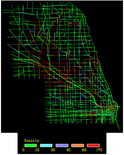
Figure 164. Illustration. Simulated network density for scenario 3 at 9:30 a.m.
Figure 165 through figure 168 show the comparison of link-specific speed and flow distribution over the simulation time from 5 to 11 a.m. similar to the one in figure 159 through figure 162. It can be seen that the flow is slightly lower in the beginning due to the demand reduction, but the free-flow speed can be obtained for a longer period of time. Whereas in scenario 1, the congestion reduces the speed to 10 mi/h by 10:30 a.m., and the speed with demand reduction maintains slightly higher for another 20 min. Similar observations can be made by comparing the flow distributions, where scenario 3 shows slightly higher volumes from 9:30 a.m. on.

Figure 165. Illustration. Simulated link speed distribution for scenario 2 for the Kennedy Expressway between Pulaski Road and North Cicero Avenue westbound.
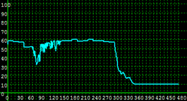
Figure 166. Illustration. Simulated link speed for scenario 3 for the Kennedy Expressway between Pulaski Road and North Cicero Avenue westbound.
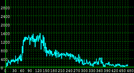
Figure 167. Illustration. Traffic volume distribution for scenario 2 for the Kennedy Expressway between Pulaski Road and North Cicero Avenue westbound.
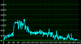
Figure 168. Illustration. Traffic volume distribution for scenario 3 for the Kennedy Expressway between Pulaski Road and North Cicero Avenue westbound.
Scenarios 4.1.1 and 4.1.2:
Scenarios 4.1.1 and 4.1.2 represent a demand management strategy on top of the natural demand reduction to inform travelers of the travel times with transit compared to the auto travel times. The two scenarios make the assumption that 50 and 100 percent of the travelers are receiving this information, respectively. The following figures only show the difference between scenarios 2 and 4.1.2, where 100 percent of the travelers are informed. Figure 163 and figure 169 illustrate the effect of the mode choice for scenario 2 compared to scenario 4.1.2 on the network density. The difference is especially visible when comparing the more congested CBD from scenario 2 to scenario 4.1.2, as the mode choice has mostly an effect on trips from and to the CBD, whereas trips outside the CBD remain nearly unaffected. In total, 7.31 percent of the to and from the CBD are projected to switch to transit under snowy condition and 100 percent information, whereas this number nearly halves when assuming 50 percent information to 3.67 percent.
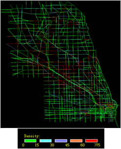
Figure 169. Illustration. Simulated network density for scenario 4.1.2 at 9:30 a.m.
Figure 170 and figure 171 show the impact of the mode choice demand strategy on the link-specific speed and flow distribution. It can be seen that the free-flow speed recovers after the breakdown before it comes to a second breakdown with an overall slightly higher traffic volume.
The average travel time decreases from 38.6 to 34.62 and 32.16 min, respectively, for scenarios 4.1.1 and 4.1.2. This corresponds to travel time reduction of 10.31 and 16.68 percent.
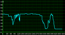
Figure 170. Illustration. Simulated link speed distribution for scenario 4.1.2 for the Kennedy Expressway between Pulaski Road and North Cicero Avenue westbound.
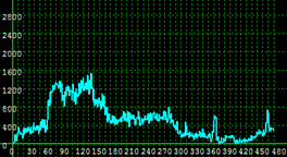
Figure 171. Illustration. Traffic volume distribution for scenario 4.1.2 for the Kennedy Expressway between Pulaski Road and North Cicero Avenue westbound.
Scenario 4.2.1 and Scenario 4.2.2:
Scenarios 4.2.1 and 4.2.2 represent a demand management strategy on top of the natural demand reduction to inform travelers of their expected auto travel time delays due to the weather condition to suggest leaving earlier or later to avoid delays. The two scenarios make the assumption that 50 and 100 percent of the travelers are receiving this information, respectively. The average expected delay for the trips is a minimum of 8 min small and a maximum of 31 min. The differences to scenario 2 are negligible, as the simulated mode shifts are too small to make an impact on the network wide traffic. Because of the small differences, the results are not shown here. The average travel time decreases from 38.6 min to 38.18 and 37.86 min for scenarios 4.2.1 and 4.2.2, respectively, which corresponds to a reduction in travel time of 1.08 and 1.91 percent.
Scenario 5:
Scenario 5 examines the effect of delaying school openings by 1 h during bad weather occurrences, as practiced in other States and cities (not including Illinois). Such policy interventions are mainly used for security reasons but also have an impact on traffic. The scenario is configured as described in the section, “Paragraph Policy Intervention: Weather-Related Delay of Schools” and illustrates the impact of such a policy on a median snow day on the network performance. School-related trips make up 8.9 percent of the traffic volume during the simulated morning hours, and its departure time distribution is much narrower distributed than work trips in the same time period. By shifting school related trips an hour later, the peak traffic can be flattened out, and the resulting difference in network densities are illustrated in figure 163 and figure 172.
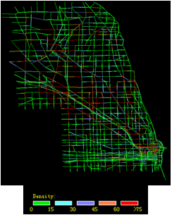
Figure 172. Illustration. Simulated network density for scenario 5 at 9:30 a.m.
Figure 173 through figure 174 show the comparison of a link speed and volume impact of school delay policy. In the comparison, it can be seen how the breakdown happens later and gets recovered soon after in the school delay policy scenario.
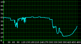
Figure 173. Illustration. Simulated link speed distribution for scenario 5 for the Kennedy Expressway between Pulaski Road and North Cicero Avenue westbound.
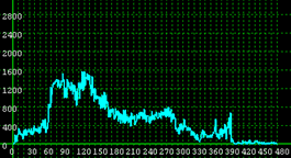
Figure 174. Illustration. Traffic volume distribution for scenario 5 for the Kennedy Expressway between Pulaski Road and North Cicero Avenue westbound.
Scenarios 6.1 and 6.2:
Scenarios 6.1 and 6.2 combine all demand management strategies and policy implementation, with 50 and 100 percent information, respectively. Figure 163 and figure 175 show the impact of scenario 2 in comparison to scenario 6.1. The speeds and densities are fully recovering the benchmark scenario 1.
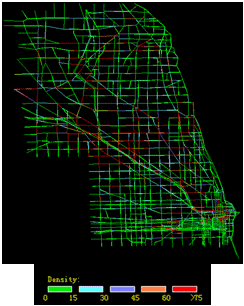
Figure 175. Illustration. Simulated network density for scenario 6.1 at 9:30 a.m.
Figure 176 and figure 177 show the comparison of a link speed and volume impact of moderate weather, natural reduction, mode choice, departure time choice, and policy intervention.
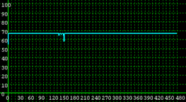
Figure 176. Illustration. Simulated link speed distribution for scenario 6.1 for the Kennedy Expressway between Pulaski Road and North Cicero Avenue westbound.
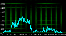
Figure 177. Illustration. Traffic volume distribution for scenario 6.1 for the Kennedy Expressway between Pulaski Road and North Cicero Avenue westbound.
Scenario Comparison and Discussion:
Figure 178 shows the accumulated percentage of out vehicles represented throughput of the network under different scenarios. One might notice that there are jumps around the 60-min mark. This is due to the time-dependent demand.
Compared to the benchmark case (i.e., scenario 1) where no snow event is present, the snow effect significantly deteriorates the network throughput if the original full demand is used and no demand management is applied (i.e., scenario 2 median snow with 100 percent demand). It can be seen that the network throughput decreases by about 7 percent due to weather at minute 120. The network performance improves as the demand level decreases. By utilizing all demand management strategies with 100 percent information, the throughput is slightly higher than the throughput of scenario 1, and with 50 percent information, the throughput is lower.
Figure 179 presents the percentage change in the average travel time and the average stop time for different scenarios relative to the benchmark case. With scenario 6.2, both measures are recovered to the level of the benchmark case.
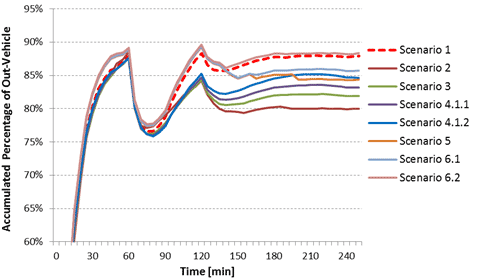
Figure 178. Graph. Accumulated percentage of out vehicle for different scenarios.
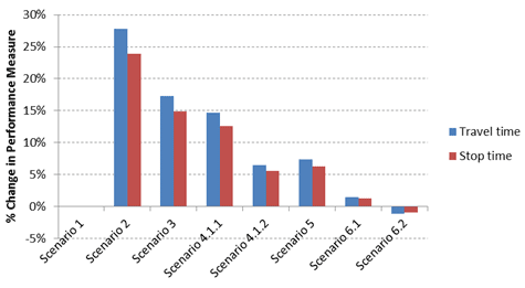
Figure 179. Graph. Changes in average travel time and average stop time relative to benchmark.
These results depict a comprehensive list of demand management and policy strategy scenarios evaluated in this study and the corresponding improvement for network-wide travelers. In general, strategies that target mode choice and effective policies that target peak spreading have good potential to improve the cost and reliability of travel by reducing travel time. By distributing better information to the traveler and comparative travel times with transit mode alternatives, travel time can be reduced while also allowing users to exert greater control over their travel schedules.
Compared to the do-nothing case (scenarios 2 and 3), the integration of behavioral models that are sensitive to policy changes and management strategies, scenarios were simulated that significantly improve the time-dependent average travel time. Information and demand management strategies are highly effective in mitigating recurrent congestion, reducing travel time, and improving travel time reliability for both critical origin-destination pairs and networks.
Limitations
The limitations of this case study are mostly due to data unavailability and missing information for calibrating parameters used in the disaggregated choice models. For the simulated responses of individuals, a fixed compliance rate is assumed. In addition, the perfect/imperfect knowledge assumption used in the sensitivity analysis is chosen arbitrarily. The assumption of the natural reduction used in scenario 2 is based on aggregated information from loop detectors and is randomly applied to the travelers. Data to estimate individual behavioral models, such as travel surveys during bad weather and good weather, would help researchers to better understand the observed reduction as well as the nature of this reduction that travelers dodge to the peripheral network as part of their route choice behavior during bad weather conditions. Furthermore, certain individual decisions can only be understood when applied within a full-blown activity based model. Such decisions (e.g., substitution patterns, location choice changes, etc.) cannot be modeled with single decision models only for a part of the day. Also, longer-term effects for bad weather situations, where the occurrence is regularly, were not included in this case study but could be part of the observed natural reduction to some extent.
Further sensitivity analysis could be made to capture the exact combination of information compliance needed to reach the presented base scenario. This sensitivity analysis could also be coupled with VMS. DYNASMART has the capabilities to include VMS strategies during the simulation as part of the route choice algorithm. Also, the relative coarse time interval of 30 min for the departure time choice model could be refined to allow finer behavioral responses in the simulated departure time choices.
Recommended Next Steps and Research
The presented case study demonstrated how to include individual behavior models to evaluate and simulate the effectiveness of particular WRTM strategies in a given network during bad weather conditions. These allow the model user/agency personnel to compare network performance overall as well as portions of the network, origin-destination pairs or user segments with and without WRTM, as well as for different WRTM strategies. This provides an understandable method to quantify and characterize the need for and effectiveness of WRTM and to communicate these impacts to other personnel, decisionmakers, and system users as part of demand management strategies. This study conveys both the dynamic nature of the information, the network context, as well as the impact on users’ decisions on trip cancellation, mode choice, departure time choice, and route choices.
The simulated demand strategies needed to offset the weather-induced network performance impairment and maintain the normal conditions level of service are a combination of transit travel time information given to auto users and policy implementation to shift school openings by an hour. The reduction depends on the nature, intensity, severity, and duration of the weather conditions. This information provides a practical target to attain through various information dissemination measures, activity cancellation or rescheduling measures, and possible incentive schemes to reach the desired level of reduction and shift in demand. The case scenario presented here shows one possible weather condition and a demand strategy of how to reduce the demand to reach LOS comparable to clear weather conditions. With different effort in dissemination of information to the auto user, a certain level of information, knowledge, and awareness could be reached to change mode and departure time decisions of individuals to reach the benchmark LOS. Models to estimate information and attitude/awareness dissemination are still relatively new to this field, but agent-based models as presented in chapter 6 are promising to model and simulate such scenarios.
In all areas, the responses of travelers to information, messaging, guidance, and controls are an essential ingredient to the overall effectiveness of management strategies. These decisions play a central role in this case study. While the methodology applied in this study provides the necessary framework and structure to capture these decisions and their evolution, it became clear during the study that a stronger observational basis is needed with regard to what users actually do in bad weather and under different interventions. The study team believes that a targeted application with tracking of a sample of users would contribute significantly to the ability of agencies to effectively deploy WRTM. Such a behavior tracking study that would allow observation of actual user responses to WRTM strategies, with particular focus on demand management strategies, would fill the data gap and minimize the assumptions, which have to be made for simulating best strategies. As noted, the lack of behavior tracking studies is an important gap in existing knowledge and a critical opportunity from the standpoint of agencies’ abilities to mitigate inclement weather. The results would be incorporated in the presented methodology to improve its ability to predict ways to attain desired demand reduction targets.
In large metropolitan areas, it is also important to incorporate alternative transportation modes in the WRTM analysis, as shown in this case study. In the simulation of the Chicago, IL, network under snowy conditions, public transit plays an important role in providing and maintaining mobility.
This case study also showed that different strategies are not additive in their impacts, and a best combination needs to be carefully determined for specific weather conditions.
Travel Behavior Variability and Intervention Following Active Traffic Management System (ATMS) Case Study
This section describes research performed on the Interstate 5 corridor in Seattle, WA, following the introduction of an automated ATMS on the corridor. It provides a summary of how information interventions are related to travel behavior variability and examines conditions of variability and demand. The other potential benefits associated with ATMS investments, such as improvements in safety, reductions in delays, and greenhouse gas emissions through speed harmonization, ramp metering, and other traffic management techniques were discussed previously in this chapter.
In the course of the research, variability in weather conditions was found to significantly influence some travel behaviors. Though weather conditions are not typically reported in the ATMS data (except for unusual circumstances), the effects of variable weather conditions are important in evaluating the larger context of the ATMS operational effects.
The purpose of this study has been to examine facility users’ reactions to information (specifically ATMS-transmitted congestion, weather, and incidents information and operational guidance) provided by VMSs and supplemented by other freeway management techniques such as ramp metering. In this context, there are a number of behavioral dimensions that can be examined that affect behavior.
The ATMS system is an additional freeway management strategy that has not been widely used in the United States. Studying a corridor that has had a system in operation for some time allows for the recording of behavioral choices by travelers in the corridor who have had a chance to use the real-time information and adjust their behavior in response to the corridor’s operations.
Program Interventions on Northbound Interstate 5 Corridor in Seattle, WA
Interstate 5 is the westernmost freeway that runs the length of the continental United States. The freeway traverses California, Oregon, and Washington. It also traverses the middle of several major metropolitan areas, including San Diego, Los Angeles, and Sacramento, CA; Portland, OR; and Seattle, WA.
Within the Seattle, WA, area, Interstate 5 is the major north-south freeway. As the major freeway, much of the alignment has four or five lanes in each direction as well as an HOV lane through much of the corridor.
The segment of Interstate 5 studied for this research is the northbound segment between Boeing Field and Interstate 90, almost entirely within the city limits of Seattle, WA. This portion of the corridor is recognized for having significant congestion throughout multiple hours of many weekdays as a result of merging traffic from Interstate 90. There are also lane reductions that occur with the opening and closing of the Interstate 5 reversible lanes that begin downtown. Finally, multiple movements as drivers enter and leave the local street system in the downtown area can contribute to congestion in this corridor segment.
To manage this congestion over the last few decades, the Washington State Department of Transportation (WSDOT) has implemented several tools to inform drivers of impending congestion. Improvements began by initiating ramp metering in the corridor. Other tools used include destination travel time signage and an ATMS that reports upstream warnings of traffic congestion as well as variable speed limits by lane. The primary purpose of the ATMS system was to reduce the occurrence of vehicle collisions and the related problem of additional non-recurring congestion. These signs are located on a series of gantries over the road at generally 0.5-mi spacing.
Behavioral Dimensions: Route Choice, Departure Timing, and Trip Cancellation
ATMS may influence a number of decisions that travelers make. These decisions include the following:
Data Available and Used in Case Study
Traffic Volume and Speed Data
WSDOT maintains an FTP site with 6 months of performance data on area roadways. These data are available in 20-s or 5-min increments. As this deals with comparative travel demand choices, the 5-min data are the most applicable.
ATMS Activation Data
The ATMS system is automated so that no deliberate human decision is required for the signs to activate. A summary of the system design is available online. The signs contain advisory messages such as “slow traffic ahead” or “reduced speed zone,” with lane-assigned variable speed limits (between 30 and 50 mi/h) automatically activated when appropriate.
WSDOT maintains an internal log of signage registered each minute for each VMS in the region, including the ATMS system. The logs contain the mileage marker of each sign or sign gantry as well as time and the message indicated at each sign.
Weather Data and Selection of Weather Days
The ASOS program is a joint effort of the National Weather Service (NWS), the Federal Aviation Administration, and the Department of Defense. ASOS is designed to support weather forecast activities and aviation operations and, at the same time, support the needs of the meteorological, hydrological, and climatological research communities.
The program maintains a record of 5-min and hourly weather conditions at Boeing Field, which is adjacent to the corridor. Weather data are summarized hourly for temperature, conditions, recorded precipitation, wind speeds, and a number of other meteorological measurements. For this study, the weather conditions and the prior hour’s recorded precipitation were the primary conditions of interest in determining travel behavior choices.
The days selected for review were between Monday, September 11, 2012, and Thursday, December 6, 2012. Fridays were excluded for being atypical work days, and Saturdays and Sundays were excluded because weekend travel is different from weekdays. In addition, November 21 and 22, 2012, were excluded because of the variation in traffic that occurs on these days. Finally, home game days of the Seattle Mariners were excluded.
The remaining days were separated into the following three categories based on type of weather condition:
Days that were clearly transitional were excluded from the sampling. The days selected for these typologies are shown in table 29.
Table 29. Boeing Field weather data.
| Date | Day | Precipitation Total (inches) | Recorded Hours Precipitation | Precipitation Hours (5 a.m.–9 p.m.) |
Category of Day |
| 9/10/12 | Monday | None | None | None | Dry |
| 9/11/12 | Tuesday | None | None | None | Dry |
| 9/12/12 | Wednesday | None | None | None | Dry |
| 9/13/12 | Thursday | None | None | None | Dry |
| 9/17/12 | Monday | None | None | None | Exclude Seattle Mariners |
| 9/18/12 | Tuesday | None | None | None | Exclude Seattle Mariners |
| 9/19/12 | Wednesday | None | None | None | Exclude Seattle Mariners |
| 9/20/12 | Thursday | None | None | None | Dry |
| 9/24/12 | Monday | None | None | None | Dry |
| 9/25/12 | Tuesday | None | None | None | Dry |
| 9/26/12 | Wednesday | None | None | None | Dry |
| 9/27/12 | Thursday | None | None | None | Dry |
| 10/1/12 | Monday | None | None | None | Exclude Seattle Mariners |
| 10/2/12 | Tuesday | None | None | None | Exclude Seattle Mariners |
| 10/3/12 | Wednesday | None | None | None | Exclude Seattle Mariners |
| 10/4/12 | Thursday | None | None | None | Dry |
| 10/8/12 | Monday | None | None | None | Exclude Columbus Day |
| 10/9/12 | Tuesday | None | None | None | Dry |
| 10/10/12 | Wednesday | None | None | None | Dry |
| 10/11/12 | Thursday | None | None | None | Dry |
| 10/15/12 | Monday | 0.3 | 12 | 11 | Drizzle |
| 10/16/12 | Tuesday | None | None | None | Dry |
| 10/17/12 | Wednesday | None | None | None | Dry |
| 10/18/12 | Thursday | 1.04 | 4 | 2 | Transitional |
| 10/22/12 | Monday | 0.35 | 10 | 9 | Rain |
| 10/23/12 | Tuesday | T | 4 | 2 | Drizzle |
| 10/24/12 | Wednesday | 0.19 | 17 | 10 | Drizzle |
| 10/25/12 | Thursday | None | None | None | Dry |
| 10/29/12 | Monday | 0.7 | 9 | 5 | Rain |
| 10/30/12 | Tuesday | 1.39 | 19 | 15 | Rain |
| 10/31/12 | Wednesday | 0.72 | 16 | 11 | Rain |
| 11/1/12 | Thursday | 0.39 | 10 | 5 | Rain |
| 11/5/12 | Monday | 0.05 | 1 | 0 | Dry |
| 11/6/12 | Tuesday | 0.01 | 1 | 1 | Dry |
| 11/7/12 | Wednesday | None | None | None | Dry |
| 11/8/12 | Thursday | None | None | None | Dry |
| 11/12/12 | Monday | 0.16 | 6 | 2 | Drizzle |
| 11/13/12 | Tuesday | 0.19 | 9 | 4 | Drizzle |
| 11/14/12 | Wednesday | None | None | None | Dry |
| 11/15/12 | Thursday | None | None | None | Dry |
| 11/19/12 | Monday | 2.38 | 15 | 11 | Rain |
| 11/20/12 | Tuesday | 0.23 | 5 | 4 | Rain |
| 11/21/12 | Wednesday | 0.59 | 14 | 9 | Excluded (Thanksgiving) |
| 11/22/12 | Thursday | 0.02 | 2 | 0 | Excluded (Thanksgiving) |
| 11/26/12 | Monday | None | None | None | Dry |
| 11/27/12 | Tuesday | None | None | None | Dry |
| 11/28/12 | Wednesday | 0.12 | 8 | 8 | Drizzle |
| 11/29/12 | Thursday | 0.12 | 14 | 11 | Drizzle |
| 12/3/12 | Monday | 0.77 | 21 | 13 | Rain |
| 12/4/12 | Tuesday | 0.53 | 21 | 15 | Rain |
| 12/5/12 | Wednesday | None | None | None | Dry |
| 12/6/12 | Thursday | 0.07 | 9 | 7 | Drizzle |
| Source: Boeing Field Weather Station Data, NWS | |||||
Transit Demand Data
Daily transit boardings were available for a number of bus, light rail, and commuter rail services that operate in the corridor under monitor by the Sound Transit District. An automated passenger counting (APC) system recorded northbound data on Sound Transit buses (Routes 577, 590, 592, 593, 594, 595, and 596) that operate on the Interstate 5 corridor and commuter rail services that operate on railroad tracks adjacent to the corridor for the study period. The link light rail system, which generally follows the corridor, did not have a recording of each transit trip, so a surrogate measure of the recorded trips from passengers’ transit cards at the three southernmost stations (Sea-Tac Airport, Tukwila International Boulevard, and Rainier Beach) were used to determine variability. Additionally, King County Department of Transportation Metro Transit Division operates two routes in the corridor (routes 101 and 150), but the APC equipment on these routes was not comprehensively installed, so that these data were not examined.
In addition, there were two transit-related system changes that occurred that were accounted for in the mode choice data only. On September 29, 2012, the free-fare zone for transit riders in downtown Seattle was discontinued. That potentially could have affected the way that data were registered in the corridor (even though the fare policy change did not directly affect transit riders in the corridor). A second transit occurrence was the extending of the Sounder commuter rail from downtown Tacoma to South Tacoma and Lakewood station on October 8, 2012. For these reasons, mode choice data before October 8, 2012, were excluded.
Findings
The research yielded findings for a variety of circumstances. Note that these findings point to variability in observed aggregate travel conditions rather than individual travel behavior. As a result, the findings represent key observations, but the actual causes of the variability can only be interpreted. Future research should focus on behavioral tracking studies along ICM and ATMS corridors to capture individual responses over time.
Inertia/Trip Cancellation
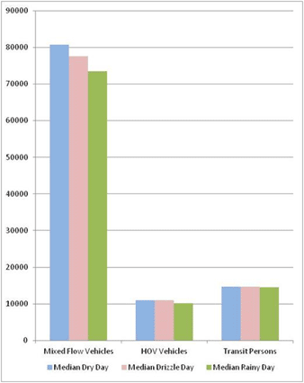
When examining the overall demand in the corridor, it is clear that there is variation in demand that is affected by weather conditions. To examine this, the median days of the three weather types were examined. The data examined in the corridor suggest that the total demand does vary with weather conditions. The findings are summarized in table 30 and illustrated in figure 180. For daily travel, there is a significant drop in demand for rainy days and a less significant drop for drizzle days.
Table 30. Summary of daily demand (October 10, 2012, to December 6, 2012).
| Attribute/ Weather |
Mixed Flow Vehicles | HOV Vehicles | Transit Persons |
| Median Day Type | |||
| Dry | 80,739 | 10,944 | 14,736 |
| Drizzle | 77,497 | 10,991 | 14,697 |
| Rain | 73,479 | 10,102 | 14,515 |
| Percent—Standard Deviation ÷ Mean | |||
| Dry | 3 | 5 | 3 |
| Drizzle | 1 | 4 | 1 |
| Rain | 4 | 4 | 3 |
| Percent of Dry Days | |||
| Dry | 100 | 100 | 100 |
| Drizzle | 96 | 100 | 100 |
| Rain | 91 | 92 | 99 |
| Percent of Total Trips (not adjusted for auto occupancy) | |||
| Dry | 76 | 10 | 14 |
| Drizzle | 75 | 11 | 14 |
| Rain | 75 | 10 | 15 |
| Sources: DKS Associates, 2013 using data from WSDOT and Sound Transit. | |||
Source: DKS Associates
Figure 180. Graph. Summary of daily demand.
Destination Choice
The techniques applied did not produce results that indicated that information provided to travelers produced changes in destination choice. It is possible that daily reduction in travel could be due to destination choices, but it is more likely that trip cancellation created by more inertia not to travel was the cause of the observed travel reduction.
Mode Choice
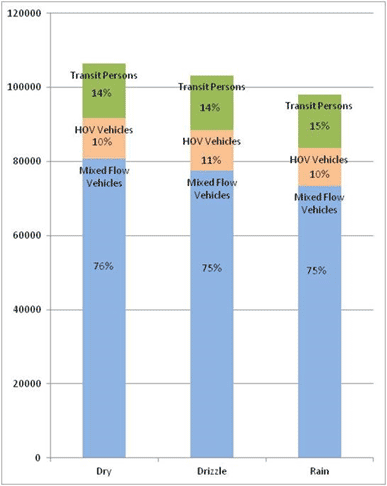
The same data in figure 180 can be examined to suggest where daily mode choice changes might be occurring. There is clearly a reduction in traffic in mixed flow lanes, but corresponding increases in the daily demand in the HOV lane and in transit boardings are not demonstrated. This suggests that the primary reduction in activity is due to trip cancellation rather than shifting to another mode. Figure 181 summarizes the different mode shares for each type of day using medians from the various data sources. It should be noted that this figure does not account for the vehicle occupancies by mode, as these are not recorded in the analyzed datasets.
Source: DKS Associates
Figure 181. Graph. Comparison of transit usage to Interstate 5 northbound traffic.
Time of Day Choice
The data presented in figure 180 for mixed flow traffic have been disaggregated for 10-min periods throughout the day. The data for the median dry, drizzle, and rainy days are summarized by time-of-day in figure 182 through figure 184. To illustrate the magnitude of variability in each type of day, the graphs in the figures also include standard deviations. Because there are between 7 and 11 days included in the sampling, the applicability of the more statistically appropriate variable of 15 and 85 percent is not used. Instead, the standard deviation is used for illustrative purposes.The location in the corridor that was examined was south of the Swift Avenue/Albro Place off-ramp (Boeing Access Road off-ramp) at monitoring location mile post 157.42. At this location, the effects of queuing in the corridor often are not reflected in the traffic speeds recorded. Mixed flow and HOV volumes are combined at this location.
Figure 182 shows a median dry day. As is apparent from the graph, the early morning conditions are relatively constant, exhibiting little variation. The highest volumes occur in the morning peak period, with a maximum median of about 1,250 vehicles for the 10-min period (the morning peak period contains two peak volume periods as a result of arriving shift workers at nearby facilities). As the day progressed, some variability was observed later in the morning peak after 9:00 a.m., suggesting that the end of the morning peak period had variable congestion and that vehicle flows responded to this. Slight variability continued through the remainder of the day. Traffic generally remained steady at about 800 to 900 vehicles during each 10-min period. This continued to about 5:30 p.m.
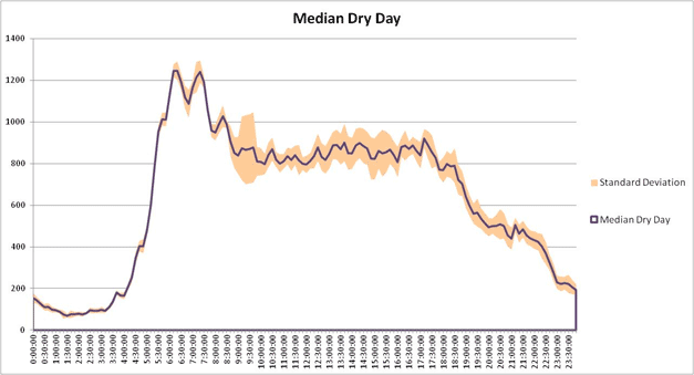
Source: DKS Associates
Figure 182. Graph. Median dry day volumes by time of day—south of Boeing Access Road off-ramp.
As is shown in figure 183 for the median drizzle day, the overall traffic demand began to decrease, but this decrease was slight through most of the day. The demand appears much more variable, although the median is comparable for dry days for many of the time periods. The second highest morning peak traffic median at about 7:20 a.m. is shown to be well below 1,200 vehicles. Another notable demand change is toward the end of the afternoon peak period. The median demand at 6:30 p.m. was about 700 vehicles for a 10-min period, while this was above 750 on dry days.
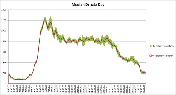
Source: DKS Associates
Figure 183. Graph. Median drizzle day volumes by time of day—south of Boeing Access Road off-ramp.
Rainy days showed significant decreases in demand as indicated in figure 184. The morning peak at about 6:30 a.m. had only about 900 vehicles for the 10-min period for mixed flow lanes. The median day showed volumes about or below 800 vehicles for much of the day, and the median demand time remained well under 800 vehicles for the 10-min period. The most notable demand change was toward the end of the afternoon peak period. An examination of the 6:30 p.m. occurrences showed that a median rainy day had about 600 vehicles for a 10-min period, while this was over 650 vehicles for drizzle days and 700 vehicles on dry days.
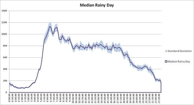
Source: DKS Associates
Figure 184. Graph. Median rainy day volumes by time of day—south of Boeing Access Road off-ramp.
Path Choice
As noted earlier, the ATMS activation appears to influence travel behavior. As the system was only visible to the drivers on the roadway, the effects of the ATMS would seem to be most directly related to path choice.
To illustrate how this behavior varies, a comparison of the demand on the Interstate 5 north mainline at the first gantry, located south of the Martin Luther King, Jr. Way and the Boeing Access Road off-ramps (part of a larger complex interchange) were closely examined. This location represents the highest off-ramp activity on the southern portion of the study corridor. Combined, these off-ramps carry between 10 and 20 percent of all the upstream mainline traffic, with especially high proportions during the morning peak hour as it serves workers at Boeing Corporation’s Boeing Field facilities.
The findings are graphically depicted in figure 185. November 12, 2012, showed relatively similar demand to the typical median drizzle day at this location. Most of the day, when the ATMS was not activated, the demands were similar between each kind of day. However, when the ATMS was activated in the morning and evening peak periods, the effects of the activation were mixed. In the morning, the activation did not appear to significantly impact the share of exiting traffic. In the afternoon peak period, the mere activation indicated that the message of traffic delays ahead resulted in an increase in off-ramp traffic above the maximum standard deviation and well above the median drizzle day. This is likely a result of morning peak period drivers needing to remain on Interstate 5 to reach destinations farther away or avoidance of high off-ramp activity at the interchange. The afternoon peak period drivers may have had fewer time constraints or were going to destinations where other paths were more reasonable.
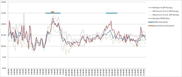
Source: DKS Associates
Figure 185. Graph. Percentage of off-ramp traffic comparing median and study drizzle day.
Conclusions
The following conclusions from this research illustrate how variability influences the way that freeway operations strategies work and that variability should be a component of traffic operations research from a behavioral perspective:
Limitations
This specific case study provides the ability to intervene in real-time mode choice behavior, so this conclusion is reasonable when applied to this corridor. Its transferability to other corridors will need to be verified before an overall conclusion that mode choice is not a significant behavioral change can be made.
The automated protocols established in an ATMS design are critical to its success, and the success in this corridor may be increased or decreased depending on the signage protocols and placements for ATMS activation. Testing of the automated protocols in this corridor will need to be examined more closely for sensitivity before it is clear what system works most effectively.
Recommended Next Steps and Research in ICM/ATIS
Forecasting methods can be enhanced by incorporating occurrences of variability in the system in some way to reflect variability in influencing factors such as weather rather than relying solely on average behaviors. Travel diaries or GPS travel survey tools for household travel behavior can be expanded to examine the effects on trip generation rates. Furthermore, APC system data can be helpful in examining mode share issues further in corridors. This may be appropriate to focus on the proportions of trips that normally occur at those times, particularly non-work, non-college, and non-home-based trips.
Sensitivity studies on automated protocols yield how successful they are. Research should focus on similar types of days as weather affects demand. Measuring traveler awareness of alternatives is important not only for understanding their choices and experience, but also for capturing the influence of experience travelers in their social networks (see chapter 6).