U.S. Department of Transportation
Federal Highway Administration
1200 New Jersey Avenue, SE
Washington, DC 20590
202-366-4000
Federal Highway Administration Research and Technology
Coordinating, Developing, and Delivering Highway Transportation Innovations
| REPORT |
| This report is an archived publication and may contain dated technical, contact, and link information |
|
| Publication Number: FHWA-HRT-13-097 Date: September 2014 |
Publication Number: FHWA-HRT-13-097 Date: September 2014 |
The objective of this chapter is to present a social network-based attitude diffusion system model in the context of activity and travel choice behavior, especially in response to a new green transportation alternative. The model framework could be extended and modified to include attitudes toward other choice dimensions (e.g., mode choice, departure time choice, etc.).
Most choice behavior dimensions are explained by the individual decisionmaking entity’s socio-economic characteristics and attributes of the different alternatives to choose from. However, these are not the only variables that explain heterogeneity in the mode preferences. Following the pioneering work of Koppelman and Pas and McFadden, it has become well accepted that attitudes and perceptions play an important role in the decisionmaking process.(126,127) Attitudes and perceptions cannot be directly observed from the data and are as a result considered latent variables.
The structural equation models of attitudinal variables are integrated into choice models in order to make use of simultaneous estimation of choice and attitudinal variables.(128) These integrated models, which have been in use since the early 1980s in travel behavior studies, were later generalized into so-called hybrid choice models and popularized by Ben-Akiva et al.(129,130) They provide a general framework where attitudinal variables are considered as latent variables.
In transport research, a large literature base exists on the use of attitudinal latent variables to explain traveler behavior and choices. Golob presents a good overview of these studies.(128) Scheiner and Holz-Rau analyze the interrelation between socioeconomic characteristics, lifestyle, residential choice, and travel behavior of individuals.(131) They confirmed that lifestyle preferences play a key role in the residential choice of individuals, which in turn has an important impact on the travel mode choice. Similarly, Van Acker et al. studied how residential and travel attitudes affect residential location and travel behavior decisions using data from an Internet survey in Flanders, Belgium.(132) The study provides confirmatory evidence that car ownership is significantly affected by residential attitudes. Van Acker et al. extended the model by including interrelations between residential and travel mode choices for leisure trips.(133) The study points out that the strength of interrelation depends on the mode as well as the activity performed. It also identifies different lifestyle characteristics that result in different travel mode decisions. By comparing the models with and without lifestyle characteristics, the authors conclude that inclusion of these subjective variables results in improvement in terms of the explained variance in mode choice.
In integrated choice and latent variable models, the attitudinal variables are included as explanatory variables of the choice. Johansson et al. analyzed the effect of the latent variables of environmental preferences, safety, comfort, convenience, and flexibility on mode choice using a sample of Swedish commuters.(134) They provide insights for policymakers so as to improve the transport systems through the use of the attitudinal variables. Espino et al. studied the mode choice behavior for suburban trips by including the latent variable of comfort.(135) Abou-Zeid et al. explained the variability in individuals’ willingness to pay using individuals’ attitudes toward travel through a latent variable model.(136) They introduce a car-loving attitude and show that individuals who dislike public transport are more sensitive to the time and cost changes of public transport compared to others.
While conceptually appealing and empirically significant, incorporating attitudes in forecasting model systems has always been somewhat problematic when the target population of interest is large. Unlike measurable attributes, the latency of attitudes has made forecasting their future values especially challenging. For this reason, when applying travel choice models to predict demand in practice, it is generally assumed that the attitudes are stable and that travelers are aware of the attributes of the available alternatives. However, when new services are introduced or some attributes of the transport system are changed, not all travelers will be aware of the change to adjust their attitudes accordingly. Rather, they will learn about those changes through various information sources, including social interaction. In these cases, consideration of the new opinion generation process and the role of information diffusion in social interaction becomes an important element in the attitude updating process that determines the eventual demand for the service. Furthermore, several new policy interventions aimed at changing the habitual behaviors of tripmakers and overcoming the associated inertia associated with established routines, especially towards more sustainable (greener) alternatives, require targeting the underlying attitudes. Hence, it is important to understand the mechanisms by which attitudes are formed, updated, and transformed, in addition to their impact on individual decisionmaking processes.
Attitudes can influence individual choices on many different levels, as discussed in the brief literature review in the previous section. However, most studies using latent variables in the context of travel behavior include lifestyle attitude variables toward or against more environmentally friendly modes in mode choice models or in longer-term decision models toward the ownership of certain transportation tools.
This section discusses the sequence of models used to disseminate information to form and influence attitudes as well as the influence of attitudes on choice models and how these choice models interrelate with other choice models.
The integration of these different models has several parts. First, information about greener or more environmentally friendly modes/travel opportunities is available and is disseminated across individuals. Second, based on this new information, a certain portion of the public can be influenced. As a result, people change their attitudes. These first and second steps heavily depend on interactions between individuals and their environment. Third, the attitude updates are used together with socio demographic variables and attributes that describe the different options in a choice set for a given decision. The decisions that are primarily and directly affected are the short- and medium-term traveler decisions shown in figure 27. This includes direct impacts of attitudes on mode choice and car ownership through the utility expressions for each choice alternative.
However, in the short, medium, and long term, attitudes can also further indirectly affect user decisions, such as activity pattern changes and accessibility as well as departure time choices and location choices. They may also affect even longer-term choices of home, workplace, and school location (not illustrated in the figure).
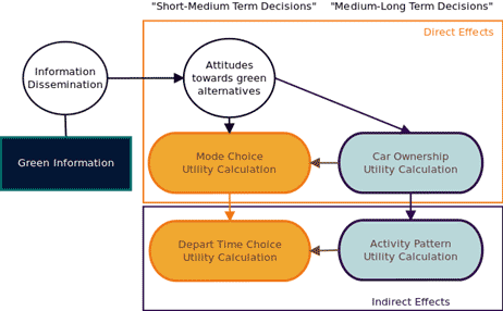
Figure 27. Illustration. Attitudes and information dissemination impact modeling
framework.
Though some studies have shown the potential of growing green transport market share and highlighted the importance of information diffusion in market adoption, there is lack of knowledge on how and to what extent that information will affect the mode choice behavior of users. When some acquaintances of an individual become commute greener fans, will he/she modify his/her own attitude or not? When a friend selects public transit or a new mobility alternative as her/his transportation mode, will that individual consider this new alternative, and will his/her mode choice change accordingly?
In this case study, the word-of-mouth mechanism was mainly used, which is modeled for large populations where people meet in small groups (e.g., pairs) with two agents to discuss their attitudes on a particular product, service, or topic. Mathematical models are developed to capture this information diffusion process.
In transportation models, it is most common to represent individual-level decisions with given attributes. These attributes determine individuals’ behaviors (e.g., choices or decisions given the characteristics of alternatives), often modeled within the random utility framework. These models are intended to provide a statistical representation of the target population. The individual behavior affected by environment attributes is calibrated at the micro level using actual data, and validation of aggregate properties in distribution against actual data. The interaction with the environment affects the decisions through many different attributes of the environment and the individual itself. Most common in transportation models is the interaction of individuals with the transportation system itself and the representation of the system through level of service attributes, which are affected by the choices of each individual and in turn affect the choices the individual makes. This iterative loop of interaction between the demand and supply models is commonly used for forecasting purposes and the evaluation of projects.
For the dissemination of information and attitudes, these kinds of models are less common and useful, as the processes rely heavily on interaction of individuals with each other. Such an interaction model is a typical feature of agent-based models, which can be described as a computational method that relies on models composed of agents that interact within an environment and with each other. Agent-based models rely on behavior rules in the form of computational models explicit about inter-agent communication and interaction, explicitly capturing processes such as learning. However, these models do not rely on statistical theories and have no such basis for prediction.
In the case of information and attitude update processes, such agent-based models are ideal, as they allow including such processes through information and interaction with other agents.
Two different kind of models, microsimulation/macrosimulation and agent-based models, can be integrated with each other by allowing the output of the agent-based models, which in this case determine the updated attitudes to be used as an input variable in utility-based choice models, as illustrated in figure 28.

Figure 28. Illusttration. Social network attitude diffusion influence process integrated into
utility-based choice models.
In the following sections, the development of an agent-based model to capture attitudes is described and then applied in a hypothetical scenario.
The agent-based model developed and described in this chapter assumes a neighborhood-based environment, within which agents interact with each other. Such an environment can be thought of as being important in influencing longer-term decisions such as mobility tool ownership. The interrelation between socioeconomic characteristics, lifestyle, residential choice, and travel behavior of the individuals has been studied by Scheiner and Holz-Rau and Van Acker et al. (See references 130–133.) Both find that residential location, lifestyles, attitudes, and travel behavior are strongly interrelated. Such an environment is created by letting agents communicate with their neighbors and influence each other (lattice social network), which then results in dynamically updating their attitudes. In such a case, the probability of communicating with a neighbor and adjusting attitudes is based on a word-of-mouth mechanism, described in the following section. The attitude adjustment calculation for each interacting pair of individuals is described in the section, “Opinion Change Model.”
Other environments to disseminate different kinds of information could be built (e.g., influences on short-term behavior could be represented within a scale-free or small world network where communication takes place trough social networking tools).
Communication Model
A basic idea of the word-of-mouth mechanism is that information is diffused from an individual to a friend or to somebody in that individual’s social network. For this reason, it is unusual that people communicate with a stranger. Thus, this mechanism implies that a threshold of selectivity exists. In reality, rich people usually have the resources to convince others regarding the merit of certain services or products. Thus, this research considers one aspect of social status, referred to as social class, as a factor in opinion formation and propagation. Following the suggestions of many sociologists, five classes were adopted: elite, upper middle, lower middle, working, and poor. Besides, the personality or charisma of people also attracts others to believe them and accept their choices in some ways. Therefore, social type, which is another social parameter, is involved. Social type characterizes an individual as an opinion leader or an opinion follower by an individual’s personality.
For this model, it was hypothesized that the role of the word-of-mouth mechanism changes by social type first and by social class second. When an information source is questionable, an individual may be less likely to revise his/her opinion during the interaction with other individuals in the future. The confidence of that individual in his/her opinion will have the same influence on opinions regardless of social class and social type. Since personalities are important in the adoption of an innovation in a community, social type has the most impact on the role mechanism.(137)
This model explains similarity concept by incorporating dissimilarity parameter and threshold parameter. The word-of-mouth dissimilarity between two communicating individuals is represented in figure 29, which is used in measuring the difference of two individuals who are trying to communicate.
![]()
Figure 29. Equation. Dissimilarity function.
Where:
i = The target individual.
j = The interacting individual.
β1, β2 and β3 = Model parameters.
SCi = Social class of individual i.
SCj = Social class of individual j.
STi = social type of individual i.
STj = social type of individual j.
Ai = Attitude strength of individual i.
Aj = Attitude strength of individual j.
The more similar two individuals are, the higher the likelihood of tending to interact or revise opinions. In this model, the researcher considers SC = {1,2,3,4,5}, ST = {1,2}, β1 = 0.2 for the difference of social class, β2 = 0.5 for the difference of social type, and β3 = 0.3 for the difference of opinion. These parameters are not calibrated but are used for illustration purposes. Data collection needs are described in the section, “Recommended next steps and research .”
The interaction threshold is speciafied in figure 30. The social type-related component follows the distribution of the diffusion of innovation theory (see figure 31) for opinion followers and increase the tolerance for opinion leaders. The social class dependent component implies the lower the social class of an individual, the larger the threshold parameter. Thus, an individual is more likely to revise his/her opinion according to the opinion of those who are more rich and powerful. When the target individual encounters other individuals and more interaction takes place, the interaction efficiency increases so that the target individual has more confidence in his/her opinion, resulting in the decrease of the threshold to interact with others.
![]()
Figure 30. Equation. Interaction threshold function.
Where:
THi = Interaction threshold for individual i.
TTi = Type-dependent tolerance of individual i.
C = Largest social class index plus 1.
Ei = Communication confidence of invididual i.
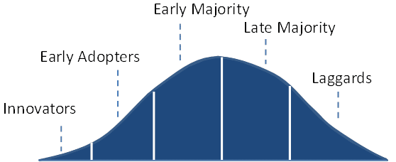
Figure 31. Illustration. Rogers’ bell curve of the innovation adoption life-cycle distribution.
The communication confidence parameter can be expressed using the following equation:

Figure 32. Equation. Communication confidence parameter.
Where:
k = Current simulation step.
J = Number of encounters in each simulation step.
L = Number of last simulation step.
t, T = Total simulation step.
Nik = Number of interactions at simulation step k.
Mik = the type-dependent memory coefficient of individual i at simulation step k.
The memory coefficient captures psychological phenomena such as the availability heuristic, whereby individuals tend to recall recent events.(138) If it is assumed that one simulation step is 1 day, memory decays in a matter of days unless individuals purposely review what they had learned. According to it, the type-dependent memory coefficient is specified as follows:
![]()
Figure 33. Equation. Type-dependent memory coefficient.
Where:
S = Relative strength of memory.
t = Total simulation step.
In figure 34, a typical exponential forgetting curve shows how information is lost over time.(139)
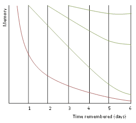
Figure 34. Graph. Forgetting curve.
When the dissimilarity is smaller than the threshold of the target individual, two individuals communicate, and the target invididual considers updating its opinion value. This situation can be discribed by the inequality in figure 35.
![]()
Figure 35. Equation. Dissimilarity inequality.
Table 16 presents the variables and their coresponding values used in the simulation experiment presented in the following sections.
Table 16. Variables and values used in the simulation experiment.
| Variable | Value |
| TTi | Inventor = 0.9; early adopters = 0.7, early majority = 0.5, late majority = 0.3, and Laggards = 0.1 |
| C | 6 |
| SCi | Social class |
| S | Opinion seeks = 0.5; opinion leaders = 1 |
| ST | 1, 2 |
For each individual, THi and STi are calculated using the value in table 16.
Opinion Change Model
When an individual decides to revise an opinion value, the opinion change model is triggered. This model utilizes an opinion-following mechanism, shown in figure 36, which is adapted by Kozuki from the car-following mechanism.(77,140)
![]()
Figure 36. Equation. Opinion change function.
Where:
Ȧi (t + T) = Change in opinion value for the target individual at time t + T.
Aj and Ai = Current opinion values of the target individual and interacting individual, respectively.
λ (ST, SC) = Impedance function that depends on social type and social class.
The new opinion value of the target individual is displayed in figure 37.
![]()
Figure 37. Equation. Opinion value function.
Where Ai (t + T) is the new opinion value and Ai (t) is the previous value.
The impedance function is composed of four mechanisms with binary variable: class-type similarity, opinion leader, opinion follower and status quo. It is represented by figure 38.

Figure 38. Equation. Impendance function.
Where:
λ = Impedance.
δi = Opinion leader status-quo bias indicator.
τi = Opinion leader indicator for individual i.
ηi = Class-type similarity for individual i.
ρ = A User-defined constant.
Υ = A user-specified constant.
Class-Type Similarity Mechanism
For the class-type simiilarity mechanism to be triggered, two interacting individuals must be similar either in social class or social type. This is described as a binary variable in figure 39.
![]()
Figure 39. Equation. Class type similarity indicator.
If the individuals are similar in social class or social type, they simply average their opinions since they carry the same social resources.
Opinion Leader Mechanism
For an opinion leader, the opinion exchanged between the leader and the other individual does not depend on the other individual’s social class. If the interacting individual is another opinion leader in a different class, the individual becomes aware of social class differences only. The following function displays these behaviors:
![]()
Figure 40. Equation. Opinion leader mechanism.
Where:
|
ρ = A user-specified constant.
Where τi specifies if the opinion leader mechanism is triggered by a binary value and ST is a binary value equal to 1 if an individual is an opinon leader, and 0 if the individual is an opinion follower. In this model example, the researcher sets α = 2 for the opinion follower and α = 0.8 for the opinion leader and Z = 2 when the interacting opinion leader is in the lower social class.
Opinion Follower Mechanism
For an opinion follower, the opinion exchanged between the follower and the other individual does not depend on the other individual’s social class. The following function displays these behaviors:
![]()
Figure 41. Equation. Opinion follower mechanism.
Where ωi specifies if the opinion follower mechanism is triggered by a binary value. In this model example, the researcher sets Қ = 2 if the interacting individual is an opinion leader and the target individual is an opinion follower and β = 2 when the interacting individual is in the lower social class.
Status Quo MechanismFigure 42 shows the status quo mechanism as a binary variable. This states that opinion leaders do not update their opinion based on opinion followers.
![]()
Figure 42. Equation. Status quo mechanism.
Attitude Update Model
For a new opinion, five attitudes, strongly disagree, disagree, no opinion, agree and strongly agree are considered. Attitude update thresholds are are follows:
The simulation experiment is based on a Netlogo modeling platform.(141) Netlogo was developed by the Northwestern University Center for Connected Learning and Computer-Based Modeling. The simulation experiment illustrates the information diffusion process through a social network in different situations. The experiment is proposed to provide a reference for the diffusion of information regarding green travel modes in a lattice neighorhood network and the possible implications of this information diffusion process on attitudes.
Design of the Experiment and Network Initialization
Based on the social class of the household, a lattice neighborhood network with four blocks is created in the Netlogo platform. Each block represents a neighborhood in the real world. Each agent in the experiment represents a family. The total number of agents in the whole network is 22,500, and each neighborhood has 5,625 families/agents. Each color represents the attitude of each agent towards green transportation modes. Violet is strongly agree, blue is agree, green is no opinion, yellow is disagree, and red is strongly disagree.
According to the distribution of the five social classes in each neighborhood (see figure 43 through figure 46), their correlation with attitude distribution (see table 17 ) and the distribution of social type (see table 18), the network is initialized where neighborhood 1 is a hypothetical high-income homogenous neighborhood. Neighborhood 2 is composed of middle upper income agents that are heterogeneous. Many low-income agents live in neighborhood 3, which represents a rather homogenous neighborhood. Neighborhood 4 is composed of middle lower income agents, which is heterogeneous.
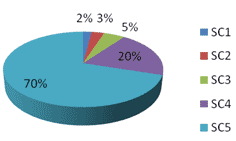
Figure 43. Graph. Social class distribution in neighborhood 1.
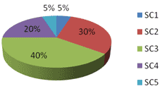
Figure 44. Graph. Social class distribution in neighborhood 2.
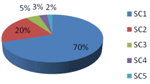
Figure 45. Graph. Social class distribution in neighborhood 3.
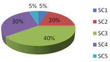
Figure 46. Graph. Social class distribution in neighborhood 4.
Table 17. Neigborhood description with social class (household income) related to attitude.
| Neighborhood | Social Class Value | Social Class Number (agents) | Distribution (percent) |
| 1 | 1 | 113 | 2 |
| 2 | 169 | 3 | |
| 3 | 281 | 5 | |
| 4 | 1,125 | 20 | |
| 5 | 3,938 | 70 | |
| 2 | 1 | 281 | 5 |
| 2 | 1,688 | 30 | |
| 3 | 2,250 | 40 | |
| 4 | 1,125 | 20 | |
| 5 | 281 | 5 | |
| 3 | 1 | 3,938 | 70 |
| 2 | 1,125 | 20 | |
| 3 | 281 | 5 | |
| 4 | 169 | 3 | |
| 5 | 113 | 2 | |
| 4 | 1 | 281 | 5 |
| 2 | 1,125 | 20 | |
| 3 | 2,250 | 40 | |
| 4 | 1,688 | 30 | |
| 5 | 281 | 5 | |
| Note: Social class: 1= Poor; 2 = Working class; 3 = Lower middle class; 4 = Upper middle class; and 5 = Elite. | |||
Table 18. Social type distribution in all neighborhoods.
| Social Type | Follower Type | Distribution (percent) |
| Opinion leader | Leader | 50 |
| Opinion follower | Innovator | 1. 25 |
| Early adopters | 6.75 | |
| Early majority | 17 | |
| Late majority | 17 | |
| Laggards | 8 |
For the neighborhood representation of the experimental scenarios in figure 47 and figure 48, there are two main assumptions in this model as follows:
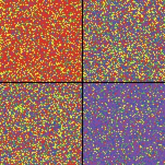
Figure 47. Illustration. Agent locations and social classes for a network before simulation
stabilization.
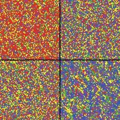
Figure 48. Illustration. Agent locations and social classes for a network after simulation
stabilization.
Basic Scenario
After the initialization of the lattice neighborhood network, the model is built on the Netlogo platform, where figure 49 shows the model interface. After the initialization, the simulation is run in Netlogo untill a stable state is reached, whereby the attitude shares among the five classes do not change anymore.
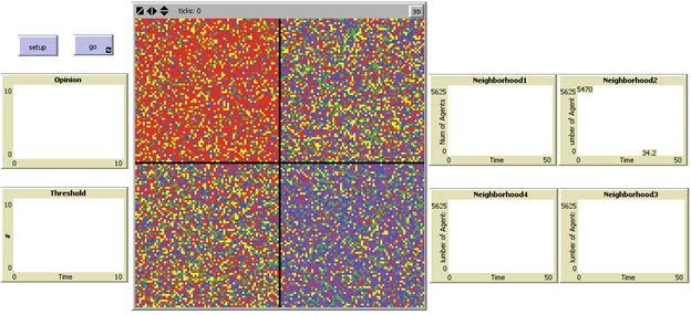
Figure 49. Screenshot. Netlogo model interface.
The attitude share distribution stabilizes with time, and its steady state is shown in figure 50 through figure 53. Each diagram describes the relationship between the number of agents and simulation time. The different colors represent the different attitudes. The statistical distribution of attitudes in each neighborhood after the simulation (base scenario) is shown in figure 54.
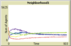
Figure 50. Graph. Number of agents with different attitudes in neighborhood 1.
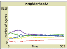
Figure 51. Graph. Number of agents with different attitudes in neighborhood 2.
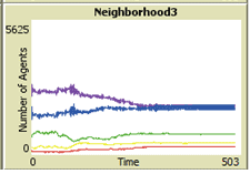
Figure 52. Graph. Number of agents with different attitudes in neighborhood 3.
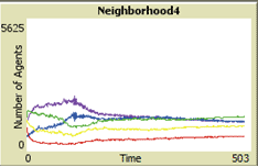
Figure 53. Graph. Number of agents with different attitudes in neighborhood 4.
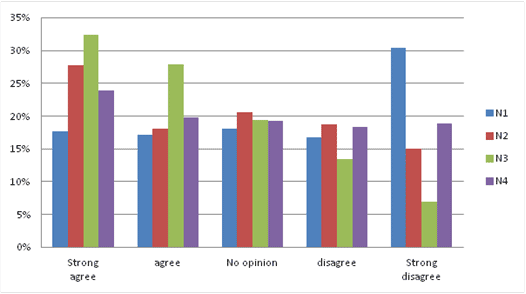
Note: N1 = Neighborhood 1, N2 = Neighborhood 2, N3 = Neighborhood 3, and N4 = Neighborhood 4.
Figure 54. Graph. Attitude distribution in neighborhoods 1–4 of base scenario.
For comparison of the neighborhoods, the following performance measures are used:
From figure 50 through figure 53, it is evident that neighborhood 1 needs the most time to converge, and neighborhood 3 can reach a stable status the fastest among the neighborhoods. Additionally, neighborhood 3 had the largest number of interactions.
Simulation Experiments and Results
With new information from outside the neighborhood, the attitudes toward more sustainable modes of transportation can be influenced. Influencing the attitudes of travellers from outside can be accomplished through a variety of ways (e.g., through targeted advertisements to influence attitudes, operational targeting via positive feedback for sustainable traveler choices, or by incentivizing the use of sustainable transport). By observing the people around them and by sharing their experience with their neighbors, the attitude diffusion process given an initial change can then be initiated. The model presented in this chapter is designed to answer the question: If we want to sustain the change in attitudes, who needs to be influenced? Additionally, how many (what fraction of) agents will change their attitude? In order to study how agents are affected by the diffusion of information under outside interventions, the following two scenarios are designed: random targeting of agents and targetting network opinion leaders. For each experiment, the stable solution described in the previous sections uses the initial network.
Random Targeting of Agents
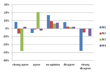
In this scenario shown in figure 55, 30 percent of agents with the attitude “strongly disagree” were selected randomly and induced to change their attitude from “strongly disagree” to “agree.” This scenario simulates a non-targeted external influence shown in figure 56.
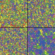
Figure 55. Illustration. Simulation results for scenario 1: random targeting simulation
results.
Note: N1 = Neighborhood 1, N2 = Neighborhood 2, N3 = Neighborhood 3, and N4 = Neighborhood 4.
Figure 56. Graph. Simulation results for scenario 1: random targeting percentage change
of attitudes.
In figure 55, outside influence effects neigborhood 3 (lower left corner) and neigborhood 1 (upper right corner) the most. Whereas in neighborhood 3, where already a majority of the agents had a positive attitude, the change cannot be sustained. The change in neighborhood 1 can be nearly sustained, as the group with “strongly disagree” attitude nearly maintain the outside change. In general, the more homogenous neighborhoods where a higher intensity of interaction is simulated are more affected by an outside intervention, whereas the heterogenous neighborhoods tend to retain the same attitude share as in the base scenario.
Figure 57 shows the compliance of the neighborhood under outside influence. The number of people rejecting the new attitude decreases in neighborhoods 1, 2, and 4. The change in neighborhood 1 is the most visible. The number of people accepting new information decreases in neighborhoods 2, 3 and 4 and increases in neighborhood 1.
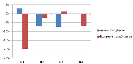
Figure 57. Graph. Percentage change of attitudes aggregated in positive and
negative attitude bins.
Targetting Network Opinion Leaders
In this second scenario, targeted influence from the outside was tested, with 30 percent of the opinion leaders selected randomly and induced to change their attitude from “strongly disagree” to “agree.” Figure 58 shows similar results as in scenario 1. However, as expected, influencing opinion leaders had a stronger impact overall. The outside influence affected the homogenous neighborhoods the most. Whereas in neighborhood 3, where already a majority of the agents had a positive attitude, the change could be sustained. The change in neighborhood 1 was sustained and expanded, as the group with “strongly disagree” attitude grew in excess of outside influence.
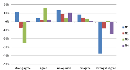
Figure 58. Graph. Percentage change of attitudes in the different neighorhoods under
scenario 2: targeting opinion leaders.
Figure 59 shows that the number of people who rejected new information under the outside influence decreased in neighborhoods 1, 2, and 4. The change in neighborhood 1 is the most striking. The number of people accepting new information decreased in neighborhoods 2 and 3 and increased in neighborhoods 1 and 4. Comparing these results with the results from scenario 1, the influence of outside factors is stronger under scenario 2.
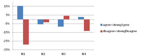
Figure 59. Graph. Percentage change of attitude aggregated in positive and negative
attitude bins.
Limitations
This case study is primarily intended as an exploratory piece, providing an outlook for future research rather than a modeling tool ready for immediate implementation. Nevertheless, information and attitudes in individual decision processes are very important and are increasingly being incorporated or considered into choice models. Especially for demand management purposes, it is important to understand the information dissemination and attitude evolution processes. Better understanding and modeling of these processes can enable agencies and policymakers to exert greater control over demand and how demand could be influenced. This does not only have to be in one direction towards more sustainable attitudes but can also be used to understand strong positive attitudes towards less sustainable behavior and how such attitudes could be reversed or mitigated.
The most significant limitation in this case study is that the models are not calibrated based on actual observations but only serve illustrative purposes to show the different processes involved in an attitude formation model and how these processes can be formulated in an agent-based modeling framework. This work underscores the large data gaps and needs in the realm of user attitudes and associated dynamic mechanisms as well as the potential value in terms of policy effectiveness of investing to deploy data gathering and user behavior observatories.
Although attitudinal questions have been integrated into recent travel surveys, these attitudes are assumed to be static and introduced in the models as being constant.(134,135) The case study in this chapter built a model to understand the processes behind these attitudes and to the research team’s knowledge. There is no data available to calibrate the developed model. Instead of relying on existing data, the model is based on concepts and processes known from literature, where similar models have been developed. As in all areas, the responses of travelers to information, messages, guidance, and controls are essential to the overall effectiveness of management strategies. Understanding the process of information dissemination and attitude formation can be an important contribution in understanding and evaluating demand management strategies, which involve information. But as attitudes and their formation dissemination may take place over a longer period, a travel behavior and attitude tracking survey would be needed to dynamically collect travel behavior and attitudinal data.
A next step would be to design an experimental survey where people would be tracked over a longer period of time and be exposed to stimuli conditioning. The survey would track how the participants learn their attitudes. Such stimuli conditioning could be through advertisements toward a particular attitude or with incentive stimuli. In a second step, participants could discuss their attitudes with the other participants around them and learn from each other.
The methodology applied in this case study provides the necessary framework and structure to capture the processes of how people learn their attitudes and could be validated and calibrated with the observation of such an experimental study and reformulated if necessary.