U.S. Department of Transportation
Federal Highway Administration
1200 New Jersey Avenue, SE
Washington, DC 20590
202-366-4000
Federal Highway Administration Research and Technology
Coordinating, Developing, and Delivering Highway Transportation Innovations
| REPORT |
| This report is an archived publication and may contain dated technical, contact, and link information |
|
| Publication Number: FHWA-HRT-11-056 Date: October 2012 |
Publication Number: FHWA-HRT-11-056 Date: October 2012 |
This section describes the technical approach to achieve the research goals. The research team captured data from a calibrated stereo rig mounted behind the rear-view mirror of a car. The data was processed at 30 frames per second using an Acadia I™ Vision Accelerator Board to compute dense disparity maps at multiple resolution scales using a pyramid image representation and a SAD-based stereo matching algorithm.(23, 24) The disparities are generated at three different pyramid resolutions, Di, i = 1, 2, …3, with D0 being the resolution of the input image. In figure 10, the pedestrian detector (PD) module takes the individual disparity maps and converts each one into a depth representation. These three depth images are used separately to detect pedestrians using a template matching of a 3D human shape model, as described in detail in section 5.2 of this report. The structure classifier (SC) module employs a combined depth map to classify image regions into several broad categories such as tall vertical structures, overhanging structures, and ground and poles to remove pedestrian candidate regions that have a significant overlap. Finally, the pedestrian classifier (PC) module takes the list of pedestrian ROIs provided from stereo modules and confirms valid detections by using a cascade of classifiers tuned for several depth bands and trained on a combination of pedestrian contour and gradient features. The rest of this section describes the algorithms implemented and the results produced by each stage.

Figure 10. Illustration. Diagram of the developed system.
The proposed system consists of a stereo rig that is made of off-the-shelf monochrome cameras and the Acadia I™ Vision Accelerator Board. The cameras are standard NTSC format 720 × 480 resolution with a 46-degree horizontal field of view.
The approach to stereo-based generic object detection framework is based on the techniques introduced by Chang et al.(25) The algorithm introduced by Chang et al. used template matching (through correlation) of pre-rendered 3D templates of objects (e.g., pedestrians and motor vehicles) with the depth map to detect objects.(25) The 3D template matching was conducted in a coarse to fine manner over a two-dimensional (2D) grid overlayed onto the local XY plane. At each grid location, a 3D template was matched to the range image data by searching around the X, Y, and Z directions according to the local pitch uncertainty due to calibrations and bumps in the road surface. Locations on the horizontal grid corresponding to local maximal correlation were returned as candidate object locations.
In the proposed method, template matching is conducted separately using a 3D pedestrian shape template in three disjoint range bands in front of the host vehicle. The 3D shape size is a determined function of the actual range from the cameras. The researchers obtains depth maps at separate image resolutions, Di, i = 1, 2, …3. For the closest range band, the researchers employed the coarsest depth map D2, for the next band level D1, and for the furthest band the finest depth map D0. This ensures that at each location on the horizontal grid, only the highest resolution disparity map that is dense enough is used. The output of this template matching is a correlation score map (over the horizontal 2D grid) from which peaks are selected by non-maximal suppression as in Chang et al.(25)
Note that this detection stage must ensure small pedestrian miss rates. As a result, a larger number of peaks obtained by non-maximal suppression is acceptable. The researchers relied on additional steps to reduce the candidates. Around each peak, the area of the correlation score map with values within 60 percent of the peak score was projected into the image to obtain the initial pedestrian ROI candidate set. This set was further pruned by considering the overlap between multiple ROIs: detections with more than 70 percent overlap with existing detections were removed. After this pruning step, a Canny edge map was computed for each initial pedestrian ROI. The edge pixels that were too far off from the expected disparity were rejected. A vertical projection of the remaining edges resulted in a one-dimensional profile from which peaks were detected using mean shift.(26) A new pedestrian ROI was initialized at each detected peak, which was refined first in the horizontal direction followed by the vertical direction to get a more centered and tightly fitting bounding box on the pedestrian. This involves using vertical and horizontal projections of binary disparity maps (similar to using the edge pixels above) followed by detection of peak and valley locations in the computed projections. After this refinement, any resulting overlapping detections were again removed from the detection list. The above approach allows detections of pedestrians and vehicles up to a range of 131.2 ft (40 m). Figure 11 through figure 14 show examples of pedestrian detection performance. In the figures, the white boxes indicate possible pedestrians, and the blue boxes indicate possible pedestrians to be further analyzed by an appearance classifier. Both true detections and typical FPs are shown. The objective of the following modules is to reduce the FPs.

|
©INRIA (See Acknowledgements section) |
Figure 11. Photo. Example 1 of pedestrian detection.(12)

|
©INRIA (See Acknowledgements section) |
Figure 12. Photo. Example 2 of pedestrian detection.(12)

|
©INRIA (See Acknowledgements section) |
Figure 13. Photo. Example 3 of pedestrian detection.(12)

|
©INRIA (See Acknowledgements section) |
Figure 14. Photo. Example 4 of pedestrian detection.(12)
A key step in the developed method for pedestrian detection is depth-based classification of the scene into a few major structural components. Given an image and a sparse and noisy range map, the goal is to probabilistically label each pixel as belonging to one of the following scene classes:
An occupied cell in the range map of a scene provides evidence for the presence of one or more of the structure classes. The structure classes outlined above typically span multiple adjacent cells in a scene with discontinuities at the boundaries of the classes. Therefore, local evidence for the presence/absence of a class can be combined with neighborhood constraints to probabilistically estimate the class labels.
The range map from the stereo does not provide enough resolution to differentiate between a group of people and a motor vehicle. As a result, the research team labels all motor vehicle-like objects as object candidates and allows the appearance-based classifier to resolve detections in these regions. These classes have been chosen to competitively label pixels among a few commonly occurring structures as a precursor to PC versus non-PC. This is in contrast to traditional detectors that directly apply PC/non-PC in which the negative examples themselves form a large set of structured classes. The research team further separates the structured classes into classes that are distinct from the pedestrian class. In this method, if large numbers of pixels can be rejected as being part of generic structural classes, the system substantially reduces the number of false hypotheses that are presented to a PC/non-PC, gaining both in performance (FP rate) and computation.
The research team performed structure classification using depth maps. An example depth map is shown in figure 15. The map is pseudo-colored with red denoting close-range objects, cyan denoting far-off objects, and black denoting missing depth. The depth map illustrates a number of issues: (1) objects appear bloated in the range map due to the stereo integration window,(2) the characteristic noise in the range values is observable as scattered fragments, and(3) the occlusion boundaries between objects are noisy.
To handle depth map errors, first, the research team defines a structure called the vertical support histogram (VSH) to accumulate 3D information over voxels in the vertical direction (see figure 15). In a given frame, the system will compute a feature vector using this structure and subsequently use the feature vector to learn the likelihood of each pixel belonging to a given structural class. Next, the team makes use of the scene-context constraints arising from the camera viewpoint by formulating the labeling problem as an MRF, where the smoothness constraints allows the team to reason about the relative positioning of the 3D structure labels in the image. This reduces error in labeling due to depth inaccuracies and gives a smooth labeling of the scene.
 through three images. The photo on the left shows people walking on a sidewalk. There are red squares in the photo which represent close range objects. The middle image shows the depth map of the photo on the left. There are two green squares which represent far-off objects. The image on the right shows two vertical histograms (for the two points on the depth map) on an XYZ plane. Each histogram bin captures a different height band. The diagram illustrates a three-bin histogram.")
|
©INRIA (See Acknowledgements section) |
Figure 15. Illustration. VSH.(12)
The main problem with using Bayesian labeling is deriving a labeling L = l of image patches, ∏, using a set of image observations, r. Suppose that both the a priori probabilities of labels and the likelihood densities of r. Suppose that both the a priori probabilities P(![]() ) of labels
) of labels ![]() and the likelihood densities p(
and the likelihood densities p(![]() | r) of r are known, the best estimate one can get from these is one that maximizes MAP, which can be computed using the Bayesian rule as follows:
| r) of r are known, the best estimate one can get from these is one that maximizes MAP, which can be computed using the Bayesian rule as follows:
![]()
Figure 16. Equation. Bayesian rule.
In the above equation, p(r), which is the density function of r, does not affect the MAP solution.
The following section describes the approach to estimate the likelihood densities p(r | ![]() ) and the prior probabilities P(
) and the prior probabilities P(![]() ) for this labeling problem.
) for this labeling problem.
The likelihood densities for the structure labels are estimated by first computing VSH, determining the likelihood of the structure labels using VSH information, and modeling the smoothness inherent in scene structures. Each of these steps is described in more detail below.
The 3D scene is represented as distributions of reconstructed 3D points with respect to a ground plane coordinate system. The ground plane can be estimated using several well-known techniques applied to the reconstructed stereo points, such as in Leibe et al.(14) The ground plane (XZ in this case) is divided into a regular grid at a resolution of Xres × Zres. At each grid cell, a histogram of distribution is created of 3D points according to their heights. All the image pixels that map into a given XZcoordinate participate in that cell's histogram. The heights, or Y coordinates, of all the points in a cell are mapped into a k-bin histogram where each bin represents a vertical height range. This structure is named VSH and is denoted by V. At any given grid cell, the following equation can be used:
![]()
17. Equation. VSH for a given grid cell.
In this equation, S gi measures the support for the ith-bin of the histogram. Figure 8 shows how image points and the corresponding depth estimates are mapped to 3D distributions for an example histogram with k = 3 bins.
Three ranges are chosen to capture the typical vertical characteristics of structures of interest which result in three histograms: hlow , hmid , and hhi .
In order to compute the supports, S g, from noisy range estimates at each pixel, the researchers uses a mean-around-the-median estimate of range. If a wxh patch is defined at each pixel (X, Y), a robust range estimate is computed for each patch (in the following, pixel and patch are used interchangeably, with the idea that the context makes the sense clear). Image points, (X, Y), with the range estimate, Z, are mapped to the corresponding (X, Z) grid cell with height estimate Y. Y is used to increment the appropriate bin of VSH at (X, Z).
Each cell of the histogram is normalized by dividing with the maximum number of pixels that can project to the cell. For a cell at a distance from the camera (with horizontal and vertical focal-lengths fx and fy , respectively), the maximum number of pixels in each image row is as follows:
![]()
Figure 18. Equation. Maximum number of pixels in each image row.
The maximum number of image rows in the height-band (Hmin and Hmax) is as follows:
![]()
Figure 19. Equation. Maximum number of image rows in a specific height band.
In this equation, Hmax is determined taking into account the maximum height that is visible in the image at distance Z. This gives the normalizing factor for the cell as follows:
![]()
Figure 20. Equation. Normalization factor for each cell in which VSH is calculated.
V(X, Z) is defined in 3D space. If this 3D representation is transferred to the 2D image and augmented with the 3D height, then, at a given image patch, p, the robust range estimate Z can be used to project this patch to a footprint (collection of cells) in the XZ-grid coordinate system. An aggregate of the VSH values for the cells within this footprint serves as the total support of p. H P is defined as the average height estimate of the image pixels within the patch. Subsequently, each such p is associated with a k + 1 - D feature vector as follows:
![]()
Figure 21. Equation. Feature vector extracted from each image patch.
VSH captures the distribution of 3D points in any given scene in terms of quantized height bins. V(X, Z) is a representation of the scene in front of a camera. In order to associate each image patch with structural labels, the researchers compute the likelihoods for the augmented feature vector, rp, conditioned on the specific structural labels defined earlier.
The research team randomly sampled approximately 100 frames from sequences in typical urban driving scenarios. In each frame, structures were coarsely hand-labeled as tall vertical structures (buildings), candidate objects (pedestrians, vehicles, etc.), ground, and overhanging structures. The research team experimented with the number of histogram bins and the placement of the bin boundaries and empirically derived the three most discriminative feature components (bins in this case). Feature vectors along these three most discriminative components for all the labeled patches rp are shown in figure 22, with different colors denoting different ground truth labels. The bin boundary values for these bins are in table 2. The resolution was 12 × 16 pixels. This separation is not surprising and can be explained as follows:

Figure 22. Illustration. Two views of the feature space showing the distribution of vectors from which the class conditional likelihoods are estimated.
| XY Histogram (meters) | MRF | |||||
| Xres | Zres | hlow | hmid | hhi | Zn | ρbp |
| 0.1 | 0.1 | 0 to 2 | 2 to 4 | 4 to 8 | 0.1 | 1.0 |
1 ft = 0.305 m |
||||||
Figure 23 through figure 26 show the various steps of the likelihood density estimation process for one frame. Note that, in particular, the vertical structure likelihoods in figure 26 capture the visible extent of the buildings all the way to the base, a task that is difficult to achieve with a simple heuristic on H.

|
©INRIA (See Acknowledgements section) |
Figure 23. Photo. Likelihood density estimation of original (left) and labeled structures (right) showing buildings and candidate objects. (12)
 images. The image on the left image shows VSH for the low vertical band (hlow), the middle image shows VSH for the middle band (hmid), and the right image shows VSH for the high vertical band (hhi).")
Figure 24. Illustration. Top view of VSH components: hlow (left), hmid (center), and hhi (right).
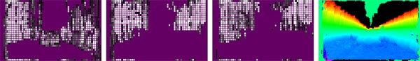
Figure 25. Illustration. VSH projected on to the image (left three images) and the height of each pixel (right).

Figure 26. Illustration. Likelihoods conditioned on the four labels: candidate objects, vertical structures, ground, and overhanging structures.
The research team performed kernel density estimation on the feature space obtained in the above process to compute the likelihood densities, p(r | ![]() ), for each of the four class labels,
), for each of the four class labels, ![]() , as follows: (27)
, as follows: (27)
![]()
Figure 27. Equation. Kernel density estimation on the feature vector extracted from each image patch.
Where:
r ci = The feature vectors of all the patches.
i = The training set belonging to the class c.
![]() = A kernel function.
= A kernel function.
H = A bandwidth matrix which scales the kernel support to be radially symmetric.
In implementation, the research team defines K(u) = k(uTu) and uses the following bi-weight kernel:

Figure 28. Equation. Bi-weight kernel used in the kernel density estimation function.
The bi-weight kernel is efficient to compute, and the research team found that it had a comparable performance to more complex kernels.
In addition to the likelihoods of structural labels, the research team modeled the smoothness inherent in scene structures through MRF priors on a pair-wise basis. The a priori joint probability of labels, P(L = ![]() ), is difficult to define in general but is tractable for MRFs. If is represented as an MRF, then the prior probability, P(
), is difficult to define in general but is tractable for MRFs. If is represented as an MRF, then the prior probability, P( ![]() ), is a Gibbs distribution given by the following equation: (28)
), is a Gibbs distribution given by the following equation: (28)
![]()
Figure 29. Equation. Gibbs distribution used to model the prior probability.
In the above equation, Es(![]() ) is the cost associated with
) is the cost associated with ![]() and is modeled as a pair-wise smoothness term between neighboring patches. L can be formulated as an MRF on the grid graph represented by the patch grid, Pi, with the four-connectivity imposed by the grid structure defining the edges. This can occur if the following conditions are satisfied:
and is modeled as a pair-wise smoothness term between neighboring patches. L can be formulated as an MRF on the grid graph represented by the patch grid, Pi, with the four-connectivity imposed by the grid structure defining the edges. This can occur if the following conditions are satisfied:
These are reasonable assumptions in this scenario. For example, the identification of a patch as a building patch might depend on whether its neighboring patches are ground but has little to do with the identity of the patches far away spatially.
The next step is to define the smoothness cost, Es, from which the prior probability P(L = ![]() ) can be computed. The smoothness term can be used to model valid configurations of scene objects possible from the camera viewpoint. Thus, for each patch, its neighboring patch will be considered, and the cost of associating a pair of labels with the two patches will be defined. The neighboring patch is defined as the patch that is four-connected to this patch and is also close in its world depth, Z w. Thus, two patches, which are neighbors in the image space but distant in the world space, are treated to have no conditional dependence on each other's labeling in the MRF network. This condition essentially cuts the grid graph along depth discontinuities before the MRF framework starts any label propagation. The remaining neighbors are now depth neighbors as well, and it is easier to reason about what objects can (or cannot) be near other objects.
) can be computed. The smoothness term can be used to model valid configurations of scene objects possible from the camera viewpoint. Thus, for each patch, its neighboring patch will be considered, and the cost of associating a pair of labels with the two patches will be defined. The neighboring patch is defined as the patch that is four-connected to this patch and is also close in its world depth, Z w. Thus, two patches, which are neighbors in the image space but distant in the world space, are treated to have no conditional dependence on each other's labeling in the MRF network. This condition essentially cuts the grid graph along depth discontinuities before the MRF framework starts any label propagation. The remaining neighbors are now depth neighbors as well, and it is easier to reason about what objects can (or cannot) be near other objects.
Let p and q be two neighboring patches from the patch grid and Z wp and Z wq represent the world depths of these patches. Define a binary variable, ![]() , as follows:
, as follows:

Figure 30. Equation. Binary variable used to test the depth neighborhood of image patches.
The binary variable defined in figure 30 is used for testing depth neighborhood using a ratio threshold, Zn. The smoothness cost assigned to the patch pair (p, q) is as follows:
![]()
Figure 31. Equation. Smoothness cost associated with each image patch pair.
In the above equation, ρbp is the constant weight factor applied to the smoothness term and is set empirically, L(p) and L(q) are the labels of p and q, and D(.) is a function that measures the compatibility between those labels.
The function D(.) is defined by considering not only the labels L(p) and L(q), but also considering if patch p is a left, right, top, or bottom neighbor of patch q. The function can enforce different costs for the same pair of labels (L(p) and L(q)) if p is below q compared to if p is above q. For example, if p is a building patch and q is below p, then q can be a building, candidate object, or ground patch. However, if q is above p, then q can only be a building patch since one cannot expect to see either ground or candidate objects along the top edge of a building. Note that in the first scenario, the candidate label is included to allow a pedestrian patch close in depth to the building patch to occlude the lower part of the building. The allowed choices for L(q) would also be the same as the first scenario if p and q were horizontal neighbors. D(.) is a binary function which imposes a penalty 1 (correction was applied) if a pair of labels is inconsistent and a penalty 0 (no correction) otherwise. In implementation, the MAP estimation (see figure 16) is done with the max-product belief propagation algorithm.(29)
The PC layer consists of a set of multirange classifiers. Specifically, three classifiers are trained for distance intervals of 0 to 65.6, 65.6 to 98.4, and 98.4 to 131.2 ft (0 to 20, 20 to 30, and 30 to 40 m) where a specific layer is triggered based on distance of detected target.
This is inspired by the fact that under a typical interlaced automotive grade camera with a resolution of 720 × 480 pixels, pedestrian ROI size on image varies substantially. For example, people who are 98.4 ft (30 m) away or farther appear on image around 25 pixels or smaller. Thus, it is desirable to handle them with approaches tuned to each specific resolution variations rather than from a single classifier covering mixed resolutions.
Each of the three distance-specific classifiers is composed of multiple cascade layers to efficiently remove FPs. For the optimal performance of the target application, the classifiers are designed with different approaches (i.e., for low latency detection at short ranges and detection at farther distances).
The first classifier is designed to reliably classify high-resolution pedestrians in a computationally efficient manner. In general, for pedestrian detection approaches reported thus far, it is often required to search for optimal ROI position and size to obtain valid classification scores.(6, 10, 14) This is due to the sensitivity of classifier to ROI alignments that results from rigid local feature sub-ROI placement inside the detection window.
This result would require exhaustive search over multiple positions and scales for each input ROI. Aside from computational overhead, the classification score also becomes sensitive and often produces false negatives.
Note that there are approaches, such as codebook-based approaches, that do not require global ROI search; however, they typically show inferior performance to approaches with fixed sub-ROI.(14, 6) False negatives can also happen when pedestrians appear against a complex background (i.e., highly textured). In this case, typical image gradient-based features become fragile due to the presence of multiple gradient directions in a local image patch.
The research team addressed this issue by designing a classifier that combines contour template and HOG descriptors, which helps with local parts alignment and background filtering (see figure 32).
 through four images. Image (a) depicts a fixed sub-region of interest (ROI). There is a person walking with a white grid on top. Image (b) depicts localized ROIs from image (a). Image (c) depicts foreground masks obtained from contour matching of image (b). Image (d) depicts filtered HOG directions in green underlying the masked regions.")
Figure 32. Photo. Process of contour and HOG classification for (a) fixed sub-ROI, (b) local ROI, (c) foreground mask from contour matching, and (d) filtered HOG directions underlying masked regions.
The research team uses a collection of templates of shape contours for each local feature window. That is, each feature window (i.e., sub-ROI) contains examples of contour models of underlying body parts that can cover different variations. For example, a sub-ROI at head position contains a set of head contours samples of different poses and shapes. Figure 33 provides an example of local contour models.

Figure 33. Illustration. Example of local contour models.
Given a pedestrian ROI, each local feature window can search in a limited range and lock on underlying local body parts. In addition to computational efficiency, it can better handle local parts deformation from pose changes and shape variations. It can also overcome ROI alignment issues.
The part contour models consist of edge maps of representative examples. Each sub-ROI contains 5 to 12 such templates. Contour template matching is achieved by chamfer matching. For each sub-ROI, the chamfer score is computed for each template model. The refined sub-ROI position is then obtained from mean position of maximum chamfer scores from each template (see figure 34).
From the contour template, a foreground mask can also be composed by overlapping binary local templates at each detected position that is weighted by matching scores. The foreground mask is used as a filter to suppress noisy background features prior to classification step.
 Ctr subscript subROI open parenthesis i subscript x, y close parenthesis equals alpha times sigma of w subscript ch times open parenthesis i close parenthesis times Ctr subscript templ times open parenthesis i; I subscript ch close parenthesis. (2) M superscript FG open parenthesis i subscript x, y close parenthesis equals M superscript FG open parenthesis i subscript x, y close parenthesis plus alpha times sigma of w subscript ch times open parenthesis i close parenthesis times I subscript templ superscript Cont open parenthesis i close parenthesis.")
Figure 34. Equation. Foreground mask for the contour template.
In the above equation, 
Where:
CtrsubROI (ix,y ) = Center of local sub-ROI.
M FG = Foreground mask.
I Conttempl = Binary contour template.
Ctrtempl( i; Ich ) = Center from chamfer matching score with the ith kernel image.
Given refined sub-ROI and foreground mask, the research team applied a HOG-based classifier. The HOG feature is computed by using refined sub-ROI boxes where gradient values are enhanced by the weighted foreground mask.
Each of the three images displays the original image, the foreground mask generated from local part templates, and the resulting edge filtering. Note that local contour parts can capture global body contours at various poses from its combinations; however, this does not form a conforming pedestrian mask for negative patches.
Figure 35 shows examples of a foreground mask and negative patches on pedestrians. Columns 3, 6, and 9 in figure 35 show the results on negative data. On the pedestrian images, the proposed scheme can refine the ROI positions on top of matching local body parts and can enhance effectively underlying body contours. The mask also produces nonconforming shape and position on negative examples. This scheme produces efficient and reliable performance on relatively high-resolution pedestrian ROIs. However, as pedestrian ROI size becomes smaller, it faces a problem as contour extraction and matching steps become fragile under low-resolution images. As a result, the researchers employ conventional HOG classifier at farther distances of pedestrian ROI (less than 35 vertical pixels).

Figure 35. Photo. Foreground mask examples.
At the second and third levels, the research team uses a cascade of HOG-based classifiers. The HOG classifier proved to be effective on relatively low-resolution imageries when body contour is distinctive from the background.
Each classifier is trained separately for each resolution band. Gaussian smoothing and subsampling is applied to match target image resolution, where 25 (at 82 ft (25 m)) and 17 (at (114.8 ft (35 m)) are nominal pixel heights for the distance interval.
Note that at farther distances, the image contrast is reduced as pedestrian ROI size becomes smaller. To compensate for this reduction and to meet scene dependent low-light situations, a histogram normalization step is used that is based on histogram stretching. For each ROI, the research team applies local histogram stretching where the top 95 percent gray value histogram range is linearly extended to cover 255 gray levels. As opposed to histogram normalization, it does not produce artifacts at low contract images, yet it can enhance underlying contours.
The research team implemented a pedestrian tracking method designed to complement intermittent missing target detection and to allow further analysis of spatial-temporal feature spaces (i.e., motion cues) to enhance classification performance. Figure 36 provides an overview of the pedestrian tracker. The red box indicates the object inside it was identified as a pedestrian, and the green shading indicates the pixel region (pedestrian’s trace) that was occupied by the pedestrian in subsequent frames.

Figure 36. Photo. Overview of the pedestrian tracker.
The tracking method consists of two steps: (1) 3D feature-based camera motion estimation and (2) image correlation-based ROI tracking. The research team’s visual odometry system computes 3D motion of the camera, specifically rotation and translation of a vehicle between adjacent frames with respect to the ground plane. To compute camera motion, the system first extracts feature points on each frame where features are obtained from corner points from various scene structures. Next, the correspondences between adjacent frames are established by using random sample consensus-based point association. Given correspondences, the relative camera motion can be computed by solving the structure from motion equation.
The estimated camera motion parameter is used to predict the location of the detected pedestrian boxes on image (ROI) in the current frame. The camera motion-based prediction is important to accurately localize ROIs under large image motions such as turning.
Given the predicted location of the ROI from the previous frame (t-1), the new location in the current frame (t) is estimated by patch correlation-based tracker module. The correlation-based tracker refines ROI position by searching through multiple candidate positions and scales of the enlarged prediction window that matches the highest appearance similarity with the corresponding ROI image patch. Figure 37 provides an equation for an image correlation tracker.

Figure 37. Equation. Image correlation tracker.
In the current system, the tracker is integrated with the PD and classifier to form a closed-loop feedback architecture. The positive outputs from PC, which are the confirmed pedestrian image patches, are fed back to the tracker, and the tracker registers them as new entries and predicts and refines the changing position of ROIs for future frames. The tracked ROIs are removed from the track queue when the following occur:
Figure 38 shows a pedestrian tracker.
 to verify that the object is indeed an pedestrian. Objects classified as pedestrians are masked by a green box and tracked.")
Figure 38. Illustration. Pedestrian tracker data flow.

