Estimation of Key PCC, Base, Subbase, and Pavement Engineering Properties From Routine Tests and Physical Characteristics

PDF Version (4.44 MB)

PDF files can be viewed with the Acrobat® Reader®

CHAPTER 5. MODEL DEVELOPMENT (19)

The maximum temperature and maximum temperature range can be obtained by running the design file and deriving this input from the worksheet titled “Climate.” For the month of May, the maximum temperature and maximum temperature range for this location are 89.6 and 39.2 °F, respectively. Using these inputs, the CRCP deltaT gradient can be calculated as -1.3214 °F/inch. For the slab thickness of 8.6 inches, this is equivalent to a deltaT of -11.36 °F. This value is comparable to the -10 °F default. This input can be revised in an MEPDG file and reanalyzed to predict punchout development over time.

Erosion for CRCP Design

The erosion model in the MEPDG was developed during the calibration of the punchout distress model. The erosion model is an empirical model that is a function of the base type, the quality of the base, precipitation at the project location, and the erosion potential of the subgrade. The erosion calculation was an upgrade provided to the CRCP distress model during changes made under NCHRP 1-40D.⁽⁴⁾ This model was examined under this study and found to adequately consider several parameters known to affect erosion. It also was recognized that within the limitations of the analysis procedures of the MEPDG and available LTPP data, the model considered all parameters that can possibly be included in the model. No changes are suggested for this model. Please note that this model was not developed under the current study but simply verified for adequacy.

EI for JPCP Design

EI is a design feature input used in the faulting prediction model of JPCP. The MEPDG recommends a rating system for different base types. The CRCP erosion model was used to develop a correlation between the calculated erosion values and EI used in the calibration files of the faulting model. The correlation was poor. However, developing a new basis for the calculation of EI for each JPCP section would necessitate the recalibration of the JPCP model, which is beyond the scope of this study. No specific recommendations are therefore made for the EI model.

Stabilized Materials Models

As stated in chapter 4, the LTPP database does not contain adequate data on modulus values and index properties of stabilized materials. It was therefore not within the scope of this project to develop predictive models for most of the stabilized materials. Nonetheless, the data could be used to develop a single model for predicting the elastic modulus of LCB materials, and that model is included in this section.

LCB Elastic Modulus Model

The modulus values of stabilized materials are not contained in the LTPP database. However, the database does include the compressive strength test results for LCB materials. For the SPS-2 sections, compressive strength data are available at 14 days, 28 days, and 1 year. Additionally, version 24.0 of the LTPP database software was reviewed.⁽¹⁴²⁾ It was found that this version contains the elastic modulus data for SPS-2 sections and that the tests were conducted on samples greater than 10 years in age, which can be more or less considered the long-term elastic modulus for the material. A predictive model correlating the elastic modulus to the 28-day compressive strength can be helpful in using this as a design input. Averaging the data by each site resulted in only 11 data points.

The data available for this model were not considered adequate to establish a new model form; therefore, the most common existing model form (i.e., correlating modulus to the square root of the compressive strength) was used. The model was established as follows:

Figure 232. Equation. Prediction model 17 for E_LCB.

Where:

E_LCB = Elastic modulus of the LCB layer.

f'_{c, 28d} = 28-day compressive strength of the LCB material.

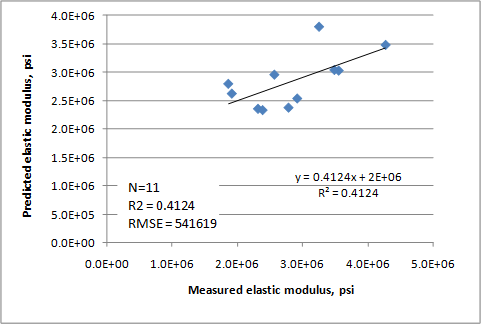
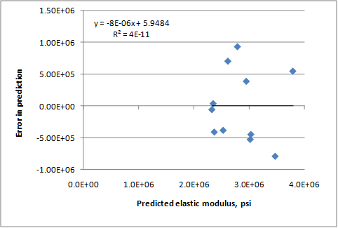
The predicted versus measured and the residual errors plots for this relationship are presented in figure 233 and figure 234, respectively. The model has an R² value of 41.24 percent, an RMSE value of 541,600 psi, and uses 11 data points.

Figure 233. Graph. Predicted versus measured for the LCB elastic modulus model.

Figure 234. Graph. Residual errors for the LCB elastic modulus model.