U.S. Department of Transportation
Federal Highway Administration
1200 New Jersey Avenue, SE
Washington, DC 20590
202-366-4000


Skip to content
Facebook iconYouTube iconTwitter iconFlickr iconLinkedInInstagram

Federal Highway Administration Research and Technology
Coordinating, Developing, and Delivering Highway Transportation Innovations

 
REPORT
This report is an archived publication and may contain dated technical, contact, and link information
Back to Publication List        
Publication Number:  FHWA-HRT-12-030    Date:  August 2012
Publication Number: FHWA-HRT-12-030
Date: August 2012


Estimation of Key PCC, Base, Subbase, and Pavement Engineering Properties From Routine Tests and Physical Characteristics

PDF Version (4.44 MB)

PDF files can be viewed with the Acrobat® Reader®

CHAPTER 5. MODEL DEVELOPMENT (20)

Unbound Materials Models

A key requirement in conducting M-E design or analysis of pavements is to estimate stresses, strains, and deflections within unbound base, subbase, embankment, and subgrade layers. The critical stresses, strains, and deflections are then used in empirical models to forecast future pavement conditions. Mostly, critical stresses, strains, and deflections within all pavement layers (including unbound base, subbase, embankment, and subgrade layers) are determined using finite element analysis (FEA) or layered elastic analysis (LEA). A key input required for determining critical stresses, strains, and deflections using LEA or FEA techniques is unbound layer material resilient modulus.

Resilient modulus is a dynamic response of unbound layer materials to continuous dynamic loading of a pavement by vehicles. It is defined as the ratio of the repeated axial deviator stress to the recoverable axial strain and is determined in the laboratory by means of a triaxial testing. Because resilient modulus is sensitive to the stress state the unbound material is subjected to (combination of confining stress ([any value]) and deviator stress ([any value])), testing typically is done over a range of confining and deviator stresses. A mathematical model is then fitted to the resilient modulus and confining and deviator stress data for use in estimating resilient modulus for any reasonable combination of confining and deviator stresses.

Developing correlations between resilient modulus and basic unbound granular/coarse-grained and fine-grained materials for use in pavement analysis and design was one of the objectives of this study. As with the other models described in this report, the LTPP database contained adequate data to develop a resilient modulus model for unbound materials.

Data Assembly for Resilient Modulus Model Development

The literature review included several models developed for the use in predicting resilient modulus using unbound material index properties. From this literature review, a list was developed of all unbound material properties that impact resilient modulus and thus could potentially be included in a resilient modulus prediction model.

Unbound material properties of interest, along with resilient modulus data required for model development as determined through the literature review, were obtained from the LTPP database and assembled in a model development database. Also included in this database were actual resilient modulus test results and the range of confining and deviator stresses at which resilient modulus was determined.

Assembly of Resilient Modulus Model Development Database

Individual LTPP material database tables were merged to develop the resilient modulus model development database. Because the LTPP database is a relational database (i.e., it is composed of separate but related data tables), data assembly was performed by linking data stored in a simple row/column format in tables using unique primary keys to identify LTPP test sections or projects. For many of the data tables, the primary keys were the combination of STATE_CODE, SHRP_ID, and CONSTRUCTION_NO.

The next step was to determine the AASHTO soil classification for each unbound material of the database. The gradation and Atterberg limits were used to determine the soil classification.

Data Review

The assembled data were reviewed thoroughly to identify anomalies and missing data elements, as well as to assess the reasonableness of the data. While this review was performed for all models developed, the review was more in-depth for the resilient modulus data because of the sheer size of the database and because of the potential for large model errors for relatively small data discrepancies.

Examples of plots summarizing the assembled data used to assess data reasonableness are presented in figure 235 through figure 247. The data were assembled and reviewed by each AASHTO soil class to assess if the trends in the data were reasonable.

This graph is a bar chart showing the mean percent clay fraction for unbound material types included in the data used to develop the unbound resilient modulus model. The data are categorized by the American Association of State Highway and Transportation Officials soil classification, which, starting from the left, are A-1-a, A-1-b, A-2-4, A-2-6, A-2-7, A-3, A-4, A-5, A-6, A-7-5, and A-7-6. The percent clay fraction is plotted on the y-axis from zero to 45 percent. The values plotted are also labeled on the solid bars as follows: 0.0, 3.9, 8.8, 11.8, 13.5, 2.3, 15.0, 33.7, 23.8, 38.9, and 36.8 percent, respectively.

Figure 235. Graph. Mean percent clay fraction for unbound material types included in the model development database.

This graph is a bar chart showing the mean percent clay fraction for unbound material types included in the data used to develop the unbound resilient modulus model. The data are categorized by the American Association of State Highway and Transportation Officials soil classification, which, starting from the left, are A-1-a, A-1-b, A-2-4, A-2-6, A-2-7, A-3, A-4, A-5, A-6, A-7-5, and A-7-6. The percent clay fraction is plotted on the y-axis from zero to 45 percent. The values plotted are also labeled on the solid bars and are as follows: 12.0, 23.8, 14.7, 16.7, 10.3, 13.6, 7.2, 9.9, 6.9, 9.2, and 4.5 percent, respectively.

Figure 236. Graph. Mean percent coarse sand fraction for unbound material types included in the model development database.

This graph is a bar chart showing the mean percent fine sand fraction for unbound material types included in the data used to develop the unbound resilient modulus model. The data are categorized by the American Association of State Highway and Transportation Officials soil classification, which, starting from the left, are A-1-a, A-1-b, A-2-4, A-2-6, A-2-7, A-3, A-4, A-5, A-6, A-7-5, and A-7-6. The percent fine sand fraction is plotted on the y-axis from zero to 80 percent. The values plotted are also labeled on the solid bars and are as follows: 18.0, 28.3, 43.3, 21.1, 12.5, 75.3, 24.8, 17.3, 17.5, 17.3, and 11.2 percent, respectively.

Figure 237. Graph. Mean percent fine sand fraction for unbound material types included in the model development database.

This graph is a bar chart showing the mean percent silt fraction for unbound material types included in the data used to develop the unbound resilient modulus model. The data are categorized by the American Association of State Highway and Transportation Officials soil classification, which, starting from the left, are A-1-a, A-1-b, A-2-4, A-2-6, A-2-7, A-3, A-4, A-5, A-6, A-7-5, and A-7-6. The mean percent silt fraction is plotted on the y-axis from zero to 45 percent. The values plotted are also labeled on the solid bars and are as follows: 5.9, 10.0, 15.8, 13.6, 15.8, 4.9, 41.9, 28.7, 42.0, 25.2, and 40.5 percent, respectively.

Figure 238. Graph. Mean percent silt fraction for unbound material types included in the model development database.

This graph is a bar chart showing the mean hydraulic conductivity for unbound material types included in the data used to develop the unbound resilient modulus model. The data are categorized by the American Association of State Highway and Transportation Officials soil classification, which, starting from the left, are A-1-a, A-1-b, A-2-4, A-2-6, A-2-7, A-3, A-4, A-5, A-6, A-7-5, and A-7-6. The mean hydraulic conductivity is plotted on the y-axis from zero to 8 ft/h. The values plotted are also labeled on the solid bars and are as follows: 5.669, 0.472, 0.118, 0.118, 1.181, 0.472, 0.472, 0.000, 0.236, 0.000, and 0.000 ft/h, respectively.

Figure 239. Graph. Mean hydraulic conductivity for unbound material types included in the model development database.

This graph shows the resilient modulus as a function of bulk stress. The 
x-axis shows bulk stress from zero to 100 psi, and the y-axis shows the resilient modulus from zero to 50,000 psi. The data are shown for two tests and are run on the base layer in Long-Term Pavement Performance section 45_1025. The first test is shown as solid triangles, and the second test is shown as solid squares. The data in this x-y scatter plot are shown for a bulk stress range of 15 to 95 psi.

Figure 240. Graph. Plot of bulk stress versus lab tested resilient modulus for section 45_1025 (base layer).

This graph is a bar chart showing the percent passing the Number 4 sieve for unbound material types included in the data used to develop the unbound resilient modulus model. The data are categorized by the American Association of State Highway and Transportation Officials soil classification, which, starting from the left, are A-1-a, A-1-b, A-2-4, A-2-6, A-2-7, A-3, A-4, A-5, A-6, A-7-5, and A-7-6. The percent passing the Number 4 sieve is plotted on the y-axis from zero to 120 percent. The values plotted are labeled on the solid bars as follows: 50.0, 69.3, 84.5, 67.1, 58.5, 96.6, 90.8, 92.9, 93.2, 95.2, and 
95.2 percent, respectively.

Figure 241. Graph. Percent passing No. 4 sieve for unbound material types included in the model development database.

This graph is a bar chart showing the percent passing the Number 40 sieve for unbound material types included in the data used to develop the unbound resilient modulus model. The data are categorized by the American Association of State Highway and Transportation Officials soil classification, which, starting from the left, are A-1-a, A-1-b, A-2-4, A-2-6, A-2-7, A-3, A-4, A-5, A-6, A-7-5, and A-7-6. The percent passing the Number 40 sieve is plotted on the y-axis from zero to 100 percent. The values plotted are labeled on the solid bars as follows: 21.4, 35.2, 63.2, 42.3, 41.0, 78.9, 79.7, 82.1, 83.0, 81.3, and 
88.3 percent, respectively.

Figure 242. Graph. Percent passing No. 40 sieve for unbound material types included in the model development database.

This graph is a bar chart showing the percent passing the Number 200 sieve for unbound material types included in the data used to develop the unbound resilient modulus model. The data are categorized by the American Association of State Highway and Transportation Officials soil classification, which, starting from the left, are A-1-a, A-1-b, A-2-4, A-2-6, A-2-7, A-3, A-4, A-5, A-6, A-7-5, and A-7-6. The percent passing the Number 200 sieve is plotted on the y-axis from zero to 90 percent. The values plotted are labeled on the solid bars as follows: 9.5, 13.4, 22.8, 23.4, 29.0, 5.3, 56.4, 65.6, 65.6, 64.3, and 
77.1 percent, respectively.

Figure 243. Graph. Percent passing No. 200 sieve for unbound material types included in the model development database.

This graph is a bar chart showing the liquid limit for unbound material types included in the data used to develop the unbound resilient modulus model. The data are categorized by the American Association of State Highway and Transportation Officials soil classification, which, starting from the left are A-1-a, A-1-b, A-2-4, A-2-6, A-2-7, A-3, A-4, A-5, A-6, A-7-5, and A-7-6. The liquid limit is plotted on the y-axis from zero to 70 percent. The values plotted are labeled on the solid bars as follows: 4.9, 5.6, 11.7, 28.7, 46.0, 0.0, 17.9, 49.3, 32.6, 59.2, and 49.3 percent, respectively.

Figure 244. Graph. Liquid limit for unbound material types included in the model development database.

. This graph is a bar chart showing the plasticity index for unbound material types included in the data used to develop the unbound resilient modulus model. The data are categorized by the American Association of State Highway and Transportation Officials soil classification, which, starting from the left, are A-1-a, A-1-b, A-2-4, A-2-6, A-2-7, A-3, A-4, A-5, A-6, A-7-5, and A-7-6. The plasticity index is plotted on the y-axis from zero to 30 percent. The values plotted are labeled on the solid bars as follows: 0.7, 0.9, 3.0, 14.6, 23.5, 0.0, 4.5, 2.2, 15.5, 25.8, and 27.5 percent, respectively.

Figure 245. Graph. Plasticity index for unbound material types included in the model development database.

This graph is a bar chart showing the maximum dry density for unbound material types included in the data used to develop the unbound resilient modulus model. The data are categorized by the American Association of State Highway and Transportation Officials soil classification, which, starting from the left, are A-1-a, A-1-b, A-2-4, A-2-6, A-2-7, A-3, A-4, A-5, A-6, A-7-5, and A-7-6. The maximum dry density is plotted on the y-axis from zero to 160 lb/ft3. The values plotted are labeled on the solid bars as follows 138.7, 131.5, 122.8, 123.4, 112.7, 110.9, 118.5, 104.0, 112.5, 95.4, and 102.1 lb/ft3, respectively.

Figure 246. Graph. Maximum dry density for unbound material types included in the model development database.


This graph is a bar chart showing the optimum moisture content for unbound material types included in the data used to develop the unbound resilient modulus model. The data are categorized by the American Association of State Highway and Transportation Officials soil classification, which, starting from the left, are A-1-a, A-1-b, A-2-4, A-2-6, A-2-7, A-3, A-4, A-5, A-6, A-7-5, and A-7-6. The optimum moisture content is plotted on the y-axis from zero to 30 percent. The values plotted are labeled on the solid bars as follows: 6.6, 8.0, 10.1, 11.1, 15.7, 11.4, 12.2, 18.7, 14.9, 23.8, and 19.9 percent, respectively.

Figure 247. Graph. Optimum moisture content for unbound material types included in the model development database.

The following conclusions were made based on the review of assembled data:

The following anomalies were identified when matching material properties data elements to Mr data for subgrade soils:


Resolving Identified Anomalies

Over half the test sections did not have all the data elements (e.g., hydraulic conductivity) required to fully characterize the pavement subgrade. However, sufficient data were available for key subgrade material properties (e.g., gradation and Atterberg limits). Data elements for which little data were available were not used in model development.

A significant anomaly was differences in subgrade soil materials used for different types of testing due to sampling location. This anomaly was resolved by matching resilient modulus data to other soil test data only when the sample location could be certified as being as close as possible (i.e., same depth/strata, same test pit, etc.).

A second anomaly was the lack of a single representative resilient modulus value for a given unbound material sample (i.e., series of resilient modulus values corresponding to a combination of deviator and confining stresses used during testing process). This situation has been resolved in the past by fitting the series of resilient modulus values corresponding to a combination of deviator and confining stresses used during testing process with a constitutive equation that models resilient modulus behavior for both granular and fine-grained materials.

As defined in chapter 3, the AASHTO Mechanistic-Empirical Pavement Design Guide, Interim Edition: A Manual of Practice proposes the constitutive equation for modeling resilient modulus behavior when subjected to various stress states the following:(1)

M subscript r equals k subscript 1 times P subscript a times open parenthesis theta divided by P subscript a closed parenthesis raised to the power of k subscript 2 times open parenthesis tau subscript oct divided by P subscript a closed parenthesis raised to the power of k subscript 3.

Figure 248. Equation. Mr.

Where:

[any value] = Bulk stress = [any value].

[any value] = Principal stress.

[any value] = Confining pressure.

Pa = Atmospheric pressure.

[any value] = Octahedral normal stress = 1/3 ([any value]).

k1, k2, k3 = Regression constants that are a function of soil properties, as defined in figure 75, through figure 77.

This model can be used for various soil types, and the model attributes (k1, k2, and k3) for a given soil type remain the same regardless of stress state. Developing models to predict constitutive model attributes for a given set of soil properties is thus an effective approach to modeling resilient modulus behavior, rather than developing models individually for each possible combination of expected stress states.


Estimating Resilient Modulus Constitutive Model Parameters k1, k2, and k3

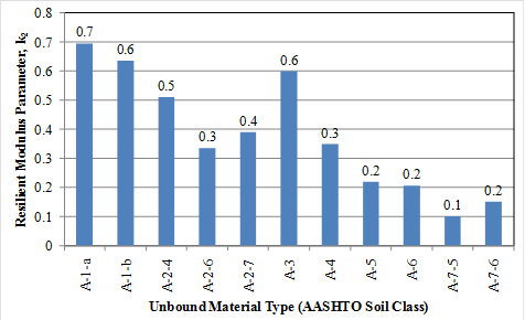
Figure 33 presents the constitutive equation that models resilient modulus behavior for both granular and fine-grained materials recommended by the AASHTO Mechanistic-Empirical Pavement Design Guide, Interim Edition: A Manual of Practice.(1) The parameters k1, k2, and k3 were calculated for all datasets based on the soil properties. Histograms showing the distribution of k1, k2, and k3 values by soil class are shown in figure 249 through figure 251, respectively.
This graph is a bar chart showing the resilient modulus parameter k subscript 1for unbound material types included in the data used to develop the unbound resilient modulus model. The data are categorized by the American Association of State Highway and Transportation Officials soil classification, which, starting from the left, are A-1-a, A-1-b, A-2-4, A-2-6, A-2-7, A-3, A-4, A-5, A-6, A-7-5, and A-7-6. The resilient modulus parameter k subscript 1 is plotted on the y-axis from zero to 1,400. The values plotted are labeled on the solid bars as follows: 862, 858, 834, 994, 1132, 792, 841, 877, 897, 677, and 845, respectively.

Figure 249. Graph. Resilient modulus parameter k1 for unbound material types included in the model development database.

This graph is a bar chart showing the resilient modulus parameter k subscript 2 for unbound material types included in the data used to develop the unbound resilient modulus model. The data are categorized by the American Association of State Highway and Transportation Officials soil classification, which, starting from the left, are A-1-a, A-1-b, A-2-4, A-2-6, A-2-7, A-3, A-4, A-5, A-6, A-7-5, and A-7-6. The resilient modulus parameter k subscript 2 is plotted on the y-axis from zero to 0.8. The values plotted are labeled on the solid bars as follows: 0.7, 0.6, 0.5, 0.3, 0.4, 0.6, 0.3, 0.2, 0.2, 0.1, and 0.2, respectively.

Figure 250. Graph. Resilient modulus parameter k2 for unbound material types included in the model development database.

This graph is a bar chart showing the resilient modulus parameter k subscript 3 for unbound material types included in the data used to develop the unbound resilient modulus model. The data are categorized by the American Association of State Highway and Transportation Officials soil classification, which, starting from the left, are A-1-a, A-1-b, A-2-4, A-2-6, A-2-7, A-3, A-4, A-5, A-6, A-7-5, and A-7-6. The resilient modulus parameter k subscript 3 is plotted on the y-axis from -0.9 to zero. The values plotted are labeled on the solid bars as follows: -0.1, -0.3, -0.6, -0.5, -0.3, -0.4, -0.8, -0.5, -0.8, -0.6, and -0.8, respectively.

Figure 251. Graph. Resilient modulus parameter k3 for unbound material types included in the model development database.

This model was fitted to all soil samples with resilient modulus available for a range of confining and deviator stresses. Model fitting was done individually for each unbound material sample in the LTPP database. For each of the soil samples, calculated k1, k2, and k3 and the constitutive equation were used to predict resilient modulus at the lab test confining and deviator stresses for comparison. The results of the comparison showed a good fit of predicted and measured resilient modulus with a high R2 value and low standard error of estimate (SEE), as presented in figure 252.
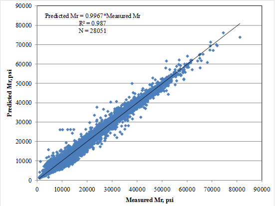
This graph shows the predicted resilient modulus (Mr) values versus the measured resilient modulus values on an x-y scatter plot. The x-axis show the measured Mr values from zero to 90,000 psi, and the y-axis shows the predicted Mr values from zero to 90,000 psi. The data are plotted using solid diamond markers. A linear trend line is also plotted. The model statistics are included as follows; predicted Mr equals 0.9967 times measure Mr, R-squared equals 0.987, and N equals 28,051.

Figure 252. Graph. Plot of measured versus calculated resilient modulus (using k1, k2, and k3 computed from constitutive model).

Resilient Modulus Model Development

The following five-step procedure using regression analysis was used to develop multiple linear regression models relating resilient modulus to unbound material properties:

  1. Determine appropriate model form.
  2. Develop inputs for regression analysis.
  3. Perform separate regression analyses for each soil class as follows:
    • Partition assembled data for use in actual model development and validation of tentative models.
    • Perform regression analysis and develop tentative models.
    • Verify tentative model by validating with “set aside” data and checking various model diagnostic statistics to determine the suitability of tentative models developed.
    • Select optimal model inputs and establish k1, k2, k3 and material properties relationship.
  4. Perform regression with full dataset and determine optimal model coefficients and diagnostic statistics.
  5. Perform sensitivity analysis and determine final model coefficients.

Details of the procedure are explained in the following sections.

Step 1: Select Appropriate k1, k2, k3 Prediction Model Form

Various forms of mathematical relationships have been used for relating constitutive model parameters k1, k2, and k3 to simple material properties. The two most commonly applied, and hence most promising, model forms are as follows:

Where ki is k1, k2, and k3. Because both of these mathematical equations have been used successfully, they were both deemed appropriate and were adopted for model fitting in this project.

Step 2: Develop Inputs for Regression Analysis

The data assembled contained all inputs required for model development. Details are as previously described.

Steps 3 and 4: Perform Regression Analyses

Numerous preliminary multivariable regression runs were performed to produce the “best” model. The goal was to determine the optimal set of independent variables (material properties) that, when included in the model, will maximize adjusted R2 values and minimize errors (SEE). Other diagnostic statistics, such as the level of significance of the regression coefficient of each independent variable, COLLIN (used to check for multicollinearity) in SAS®, and VIF were made to determine the goodness of fit for the model.

Independent variables with regression coefficients significant at the 0.05 significance level (determined through performing t-tests) were retained in the models developed. The t-test threshold was set at this level so that only variables that impacted k1, k2, and k3 were significantly included in the models. The resulting models developed through regression analysis for constitutive model parameters k1, k2, and k3 are described below.

Constitutive Model Parameter k1:

k subscript 1 equals 1,446.2 minus 4.56764 times PCTHALF plus 4.92 times LL minus 27.73 times OPTMOIST.

Figure 253. Equation. Prediction model 18 for k1.


Model statistics for k1 are as follows:

Constitutive Model Parameter k2:

k subscript 2 equals 0.45679 minus 0.00073376 times PCTNO80 minus 0.00269 times LL plus 0.00060555 times PCTGRVL plus 12.97 times D subscript 10.

Figure 254. Equation. Prediction model 19 for k2.

Model statistics for k2 are as follows:

Constitutive Model Parameter k3:

k subscript 3 equals -0.188 for fine-grained soils and k subscript 3 equals -0.153 for coarse-grained soils.

Figure 255. Equation. Prediction model 20 for k3.

Where:

PCTHALF = Percent passing 1/2-inch sieve.

LL = Liquid limit, percent.

OPTMOIST = Optimum moisture content, percent.

PCTNO80 = Percent passing No. 80 sieve.

PCTGRVL = Percent gravel fraction (0.078- to 2.36-inch size).

D10 = Maximum particle size of the smallest 10 percent of soil sample.

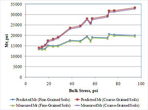
Model prediction accuracy and reasonableness were evaluated by reviewing the plot of predicted and measured resilient modulus for all individual resilient modulus test values used in model development as presented in figure 256. Note that the plot presents actual measured resilient modulus for each individual sample and stress state and resilient modulus computed using predicted k1, k2, and k3 based on actual material properties for each individual sample and the resilient modulus constitutive model and stress state. Figure 257 presents a plot of measured and predicted resilient modulus versus bulk stress for all fine- and coarse-grained materials included in model development database. Note that mean measured k1, k2, and k3 for coarse- and fine-grained materials and predicted k1, k2, and k3 using the equations in figure 70 through figure 72 and mean input values for fine- and coarse-grained materials were used for developing this plot. A review of the plots presented in figure 256 and figure 257 shows a reasonable prediction of resilient modulus.
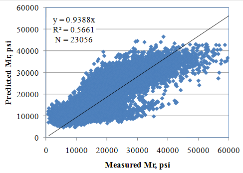
This graph shows the predicted resilient modulus (Mr) values versus the measured Mr values on an x-y scatter plot. The x-axis shows the measured Mr from zero to 60,000 psi, and the y-axis shows the predicted Mr from zero to 60,000 psi. The data are plotted using solid diamond markers. A linear trend line is also plotted. The model statistics are as follows: y equals 0.9388x, R-squared equals 0.5661, and N equals 23,056.

Figure 256. Graph. Measured versus predicted resilient modulus (using k1, k2, and k3 from figure 70 through figure 72).

This graph shows the sensitivity of the resilient modulus (Mr) model to the bulk stress for fine grained and coarse grained samples. The x-axis shows the bulk stress from zero to 100 psi, and the y-axis shows the predicted Mr from zero to 35,000 psi. The sensitivity is shown for bulk stress and ranges from 10 to 95 psi. The graph consists of four plots. The predicted Mr for fine-grained samples are represented by solid diamonds, the measured Mr for fine-grained samples are represented by solid triangles, the predicted Mr are represented by solid squares, and the measured Mr for coarse grained samples is represented by X-marks. All plots connect the markers with a solid line. The graph shows that with increasing bulk stress, the predicted Mr increases.

Figure 257. Graph. Predicted and measured resilient modulus versus bulk stress for fine- and coarse-grained soils.


Step 5: Conduct Sensitivity Analysis

The tentative models were further evaluated by conducting a comprehensive sensitivity analysis. The goal was to determine if the model behaves as expected based on engineering principles. Sensitivity analysis results are presented in figure 258 through figure 264. The results of the sensitivity analysis are summarized as follows:

Overall, the trends observed were deemed reasonable, and the proposed model was established as the recommended model for resilient modulus prediction.
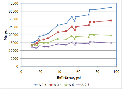
This figure is a graph showing the sensitivity of the resilient modulus (Mr) model to the bulk stress for four different American Association of State Highway and Transportation Officials (AASHTO) soil classes. The x-axis shows the bulk stress from zero to 100 psi, and the y-axis shows the predicted Mr from zero to 40,000 psi. The sensitivity is shown for bulk stress ranges from 10 to 95 psi. The four soil classes are A-1-b represented by solid diamonds, A-2-4 represented by solid squares, A-6 represented by solid triangles, and A-7-5 represented by 
X-marks. All plots connect the markers with a solid line. The graph shows that with increasing bulk stress, the predicted Mr increases.

Figure 258. Graph. Effect of material type (AASHTO soil class) on predicted resilient modulus.

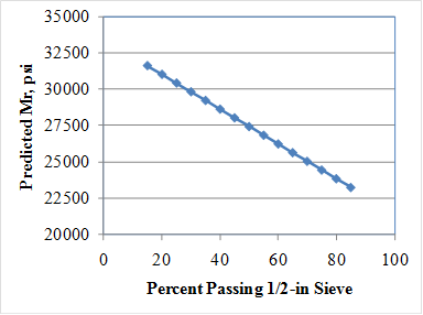
This graph shows the sensitivity of the resilient modulus (Mr) model to the percent passing the 0.5-inch sieve. The x-axis shows the percent passing from zero to 100 percent, and the y-axis shows the predicted Mr value from 20,000 to 35,000 psi. The sensitivity is shown for 15 to 
85 percent passing the 0.5-inch sieve, and the data are plotted using solid diamonds connected by a solid line. The graph shows that with increasing percent passing, the predicted Mr decreases.

Figure 259. Graph. Effect of percent passing 0.5-inch sieve on predicted resilient modulus.

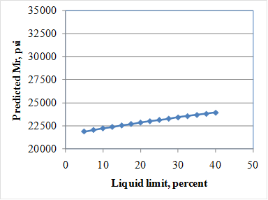
This graph shows the sensitivity of the resilient modulus (Mr) model to the liquid limit. The x-axis shows the liquid limit from zero to 50 percent, and the y-axis shows the predicted  Mr values from 20,000 to 35,000 psi. The sensitivity is shown for liquid limit ranges between 6 and 40 percent, and the data are plotted using solid diamonds connected by a solid line. The graph shows that with increasing liquid limit, the predicted Mr increases.

Figure 260. Graph. Effect of liquid limit on predicted resilient modulus.

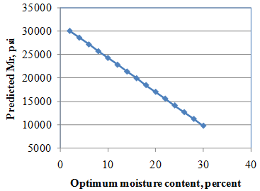
This graph shows the sensitivity of the resilient modulus (Mr) model to the optimum moisture content. The x-axis shows the optimum moisture content from zero to 40 percent, and the y-axis plots the predicted Mr values from 5,000 to 35,000 psi. The sensitivity is shown for optimum moisture content ranges between 2 and 30 percent, and the data are plotted using solid diamonds connected by a solid line. The graph shows that with increasing optimum moisture content, the predicted Mr decreases.

Figure 261. Graph. Effect of optimum moisture content on predicted resilient modulus.

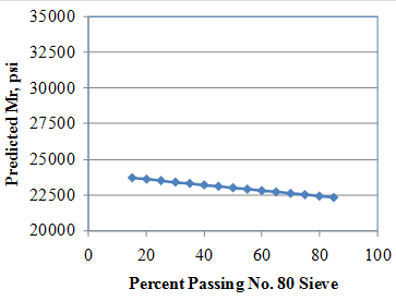
This graph shows the sensitivity of the resilient modulus (Mr) model to the percent passing the Number 80 sieve. The x-axis shows the percent passing the Number 80 sieve from zero to 100 percent, and the 
y-axis shows the predicted Mr values from 20,000 to 35,000 psi. The sensitivity is shown for 
15 to 85 percent passing the Number 80 sieve, and the data are plotted using solid diamonds connected by a solid line. The graph shows that with increasing percent passing, the predicted 
Mr decreases.

Figure 262. Graph. Effect of No. 80 sieve on predicted resilient modulus.

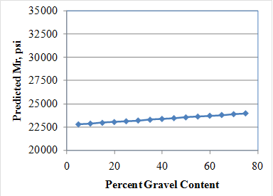
This graph shows the sensitivity of the resilient modulus (Mr) model to the gravel content. The x-axis 
shows the gravel content from zero to 80 percent, and the y-axis plots the predicted Mr values from 20,000 to 35,000 psi. The sensitivity is shown for gravel content ranges between 5 and 
75 percent, and the data are plotted using solid diamonds connected by a solid line. The graph shows that with increasing gravel content, the predicted Mr increases.

Figure 263. Graph. Effect of gravel content on predicted resilient modulus.

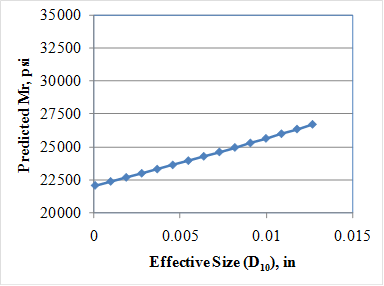
This graph 
shows the sensitivity of the resilient modulus (Mr) model to the effective size. The x-axis 
shows the effective size from zero to 0.015 inches, and the y-axis shows the predicted Mr 
values from 20,000 to 35,000 psi. The sensitivity is shown for effective sizes between zero and 0.0125 inches, and the data are plotted using solid diamonds connected by a solid line. The graph shows that with increasing effective size, the predicted Mr increases.

Figure 264. Graph. Effect of effective size on predicted resilient modulus.

Practical Guide and Software Program

The models developed under this study have been incorporated into a user-friendly software program, Correlations, which can be used independently from the MEPDG. The software, developed under this study, was developed on the Microsoft.NET platform to be compatible with the latest versions of the Microsoft Windows® operating systems. It is programmed in the C# language and uses a modern user interface library to provide a familiar look and feel. It features multiple windows on the user interface that are initially docked inside the main window. These windows can be moved separately from the main window for better viewing of the inputs or results.

The program interface features tabs for PCC, design features, stabilized materials, and unbound materials. Models that belong to each of these categories are made available through a series of radio button selections placed in an accordion control. This placement not only provides the ability to make multiple selections, but it also conserves screen space so that the results of the calculations can be placed for easy viewing. Once a model is selected, the entry area adds controls for the available inputs of the model.

Throughout the software, tooltips are used to provide feedback for each of the areas where data can be entered. Calculations occur after all necessary values have been input. Information about each of the models is available in an information window initially located at the bottom of the screen. This information is context-sensitive to the specific selections that the software user has made. Results of each calculation are displayed prominently in the results area window, initially placed on the right side of the main window.

The software program may be requested from the LTPP Customer Support Service Center at ltppinfo@dot.gov.


Federal Highway Administration | 1200 New Jersey Avenue, SE | Washington, DC 20590 | 202-366-4000
Turner-Fairbank Highway Research Center | 6300 Georgetown Pike | McLean, VA | 22101