• Construction Noise
  • Handbook
  • RCNM Version 1.1
  • RCNM Version 2.0
  • Special Report
• Measurement
• Noise Barriers
• Noise Compatible Planning
• Regulation and Guidance
• Resources
• Tire Pavement Noise
• Traffic Noise Model
• Training

Special Report - Measurement, Prediction, and Mitigation

Chapter 3 Prediction of Construction Noise

3.0 Background

The purpose of this chapter is to present a prediction methodology that can be used to estimate the construction noise levels associated with the construction of a highway. This prediction methodology serves two useful purposes.

1. It provides a mechanism for identifying potential noise impact areas prior to the start of construction.
2. It provides a mechanism for assessing the potential noise reduction resulting from certain mitigation strategies.

To completely fulfill the first purpose, the prediction methodology must provide as accurate an estimate of the construction noise level as the situation warrants. For example, during the early stages of project development, only a rough estimate of the expected construction noise effects is needed. This estimate is used to define general areas where construction noise may have an adverse effect. Conversely, a contractor preparing a bid on a project may need an accurate estimate of the expected construction noise levels. This estimate may indicate the extensiveness of abatement measures needed. This would likely influence the bid the contractor will submit.

To completely fulfill the second purpose, the prediction methodology must be sensitive to changes in the input parameters. This sensitivity allows the evaluation of those strategies for mitigating construction noise which are affected by the input parameters. Indeed, a knowledge of the relative effects of various mitigation measures will aid in the selection of the most cost effective abatement measure or measures.

The remainder of this chapter is organized into three sections. Section 3.1 presents the construction noise prediction methodology. Section 3.2 discusses how the prediction method can be used to identify construction noise impact areas. Section 3.3 deals with the evaluation of alternative measures.

3.1 Construction Noise Prediction Methodology

The basic methodology presented here for predicting construction noise is identical to that used in predicting highway traffic noise. It requires:

1. A noise metric to describe the magnitude of the construction noise level and its variation with time.
2. An emission model to determine the noise generated by the equipment at some reference distance.
3. A propagation model that shows how the noise level will vary with distance.

These three items can be related by the following expression:

L_eq equipment = E.L.+ 10 log U.F. - k log D/D₀ (3-1)

Where:

1. L_eq equipment is the A-weighted, equivalent sound level at a receptor resulting from the operation of a single piece of equipment over some time period.

2. E.L. is the noise emission level of the particular piece of equipment based on its work cycle, i.e., recall equation 2.4:

3. E.L. =L_j + E.F. @ 15.2 meters (D₀ =15.2 meters)

4. K is a constant that accounts for topography and geometric spreading.

5. D is the distance from the receptor to the piece of equipment.

6. D₀ is the reference distance at which the noise emission level was measured from the piece of equipment.

7. U.F. is a usage factor that accounts for the percent time that the equipment is in use over the time period.

Our primary interest lies in the overall construction noise level produced by the simultaneous operation of several pieces of equipment. The overall construction noise level at some point is simply the sum (on an energy basis) of the individual contributions of each piece of equipment. Mathematically, the overall construction noise level at some point is expressed as:

L_eq(h) = 10 log ⁿΣ_i=1 10^{L_eq(equipment)/10}    (3-2)

Where: L_eq equipment is given by equation 3-1.

L_eq site is the A-weighted, overall equivalent construction noise sound level obtained by summing the individual equipment noise levels on an energy basis, and n is the number of pieces of equipment included in the summation.

The accuracy of Equation 3-2 depends upon the accuracy of the input parameters. This is shown in Table 3.

*Maximum values may be specified in plans.
**Estimate based on limited data (see references 3, 6, 7, and 8).

Equation 3-2 can be used to identify potential construction noise impact areas or it can be used to evaluate various mitigation measures.

3.2 Identification of Potential Construction Noise Impact Areas

Equation 3-2 can be used to identify potential construction noise impact areas by providing an estimate of the expected construction noise level. The accuracy of this estimate is directly related to the accuracy of the input parameters. This can best be shown considering the two extreme situations, that is, where equation 3-2 provides its least accurate estimates and when it provides its most accurate estimate.

For projects not under construction, equation 3-2 can be used to provide a rough estimate of the expected construction noise levels. Equation 3-2 provides its least accurate estimate when conditions or values must be assumed for all of the input parameters. This generally occurs during the early stages of project development. In an example of this situation, the following assumptions are used.

1. One hour is selected as the time period of interest. This is reasonable since most construction equipment operates continuously for a one-hour period; the usage factor (U.F.) then becomes unity and 10 log U.F. is equal to zero.

2. Free field conditions are assumed, ground effects are ignored. Since each piece of construction equipment acts as a point source, the expression k log D/D₀ reduces to 20 log D/D₀

3. A representative noise emission level for a class of construction equipment is used. Note that E.L. =L_J + E.F., i.e., the equipment hourly sound level at 15.2 meters is the noise emission level.

4. The equipment is assumed to operate on the centerline of the highway.

With these assumptions, equation 3-2 reduces to

L_eq(h) site = 10 log ⁿΣ_i=1 10^{L_eq(equipment)/10}     (3-3)

Where:

1. L_eq(equipment)=(E.L. - 20 log D/D₀) equipment.
   L_eq(h) site is the one-hour, A-weighted, overall equivalent construction noise level, and D₀ equals 15.2 meters.

One additional problem exists with the prediction of construction noise for projects not under construction. An assumption must be made about the numbers and types of equipment at the site. It appears at this time, that the overall construction noise level is governed primarily by the noisiest pieces of equipment. The quieter pieces do not effect the overall level, but they do reduce the magnitude of the fluctuations in the noise level. Therefore, a rough estimate of the noise level need only include the noisiest pieces of equipment expected at the site. Problem No. 4 illustrates this procedure.

Problem No. 4: Consideration is being given to the construction of a two-lane road on new alignment between two towns. The project has advanced to the point where a preliminary assessment of potential construction impacts is needed. Make a preliminary rough estimate of the hourly equivalent sound level that will be generated for each construction phase. Average distance from the centerline of the road to the ROW line is 30.5m.

Solution

1. Step 1: Identify the main construction operations or phases which must be performed to complete the project. This will require a simplified construction schedule which is shown in Figure 7.

2. Step 2: Determine the types of equipment that will be needed to complete each construction phase identified in Step 1. Appendix A can be used to determine a representative noise emission level for each type of equipment.

3. Step 3: Based upon the results of Step 2, prepare a list, complete with representative noise emission levels, of the two noisiest types of equipment that will be used in each phase. This list is shown in columns B and C, Table 4.

4. Step 4: Use equation 3-3 to compute the L_eq(h) for each type of equipment at 30.5 meters (distance to ROW line). The result of this calculation in column E, Table 4.

5. Step 5: Compute the overall sound level for each phase using dB addition. The results are shown in Table 4, Column F.

Figure 7. Simplified Construction Schedule

¹. E.L.=L_j + E.F. where L_j is the peak value from appendix A. (A representative E.L. was chosen and it was assumed that Lm-Lb>10 dBA and ta/T=50%).

Most Accurate Estimate

Equation 3-2 provides its best estimate when all of the input data are measured, i.e., the project is under construction.

For projects under construction, some investigators have recently reported good agreement between measured and predicted noise levels (+ 2 dBA) using equations which have the general form of equation 3-2. However, to achieve this agreement, precise measurements of the following parameters were required:

1. The site topography.
2. The noise emission level of each piece of equipment used at the site.
3. The location of each piece of equipment while it was working.
4. The % of the time that the equipment was in use during the measurement period.

As a result of these measurements, accurate values were determined for the E.L., D and k for each piece of equipment operating at the construction site. This presents a problem in assessing construction noise impacts. Item 1 can be determined any time after the highway location is established. However, items 2, 3, and 4 can only be measured after construction begins. Consequently, the most accurate predictions of construction noise can only be made after construction begins. This is illustrated in Problem No. 5.

Problem No. 5: The project discussed in example 4 has now progressed to the point where contractors are bidding on the project. The special provisions require that the exterior L_eq(h) on school grounds be less than 75 dBA during school hours. A long fill is to be constructed adjacent to a school. One prospective contractor would like to use two dozers and three scrapers to construct this fill. The contractor has collected the following data on his equipment from previous projects.

Compute the noise emission level of the equipment and estimate the L_eq(h) at the school.

Solution

1. Step 1: The noise emission levels L_eq(h) at 15.2m) of the equipment is calculated by:

2. E.L.=L_j + E.F.

3. The noise emission levels are shown in table 5.

Step 2: Assign at average location to each piece of equipment. This is shown in Figure 8.

Step 3: Compute the L_eq(h) for each piece of equipment using equation 3-1 and the overall construction noise level using equation 3-2. The results are shown in table 6. The construction L_eq(h) of 80 dBA exceeds the specified goal by 5 dBA.

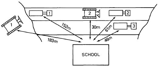
Figure 8: Construction Site

The 80 dBA value in column F was obtained by dB addition. The value could also have been determined by:

L_eq(h) site = ΣL_eq(h) equipment
= 10 log Σ 10^6.1 + 10^7.9 + 10^6.1 + 10^6.7 + 10^6.7 = 80dBA

3.3 Evaluation of Different Mitigation Strategies

Chapter 4 contains a detailed discussion of various mitigation strategies. The relative effects and effectiveness of a few of these strategies can be determined by the use of equation 3-2. This is done by holding all input parameters constant except the one affected by the particular mitigation strategy under study. Problem No. 6 illustrates how this is done.

Problem No. 6: Problem No. 5 indicates that the expected construction noise level exceeds the specified goal by 5 dBA. Evaluate different mitigation strategies that would give a reduction of 5 dBA.

Step 1: Analysis of table 6 indicates that Dozer No. 2 must be quieter if the desired goal of 75 dBA is to be met. If possible, one strategy would be to exchange Dozer No. 2 for Dozer No. 1.

Dozer No. 1: L_eq(h) = 83 - 20 log (30/15.2) = 77 dBA
Dozer No. 2: L_eq(h) = 85 - 20 log (183/15.2) = 63 dBA
L_eq(h) site = 10 log [ 10^7.7 + 10^6.3 + 10^6.1 + 10^6.7 + 10^6.7 ] = 78.1 dBA

Continued

The expected noise level exceeded the goal by 3 dBA. This strategy, by itself, is not enough.

Step 2: One mitigation strategy would be to replace Dozer No. 2. What would be an acceptable noise emission level for the replacement dozer 30 meters from the school? To answer this question, set the overall construction noise level equal to 75 dBA in equation 3-2 and solve.

L_eq(h) site = 10 log Σ 10 ^{L_eq(equipment)/10}
75 dBA = 10 log [ 10^x/10 + 10^6.3 + 10^6.1 + 10^6.7 + 10^6.7 ]
75/10 = log [ 10^x/10 + 10^7.1 ]
10^7.5 - 10^7.1 = 10^x
10^7.28 = 10^x/10         7.28 = x/10
    3       L_eq(h) = 73 dBA at 30 meters.
L_eq(h) equipment = E.L. - 20 log (D/D₀)
73 dBA = E.L. - 20 log (30/15.2)
E.L. = 73 + 6 = 79 dBA

Conclusion: This strategy accomplishes the desired goal.