
This section describes the acoustical considerations associated with highway noise barrier design, beginning with a brief technical discussion on the fundamentals of highway traffic noise.
Highway traffic noise originates primarily from three discrete sources: truck exhaust stacks, vehicle engines, and tires interacting with the pavement. These sources each produce sound energy that, in turn, translates into tiny fluctuations in atmospheric pressure as the sources move and vibrate. These sound pressure fluctuations are most commonly expressed as sound pressure and measured in units of micro Newtons per square meter (µN/m2), or micro Pascals (µPa). Typical sound pressure amplitudes can range from 20 to 200 million µPa. Because of this wide range, sound pressure is measured on a logarithmic scale known as the decibel (dB) scale. On this scale, a value of 0 dB is equal to a sound pressure level (SPL) of 20 µPa and corresponds to the threshold of hearing for most humans. A value of 140 dB is equal to an SPL of 200 million µPa, which is the threshold of pain for most humans.ref.17
The following figure shows a scale relating various sounds encountered in daily life and their approximate decibel values:
Figure 5. Decibel scale
To express a sound's energy, or sound pressure in terms of SPL, or dB, the following equation is used:
SPL = 10*log10(p/pref)2
dB
where: p is the sound pressure; and
pref is the reference sound pressure of 20 µPa
Conversely, sound energy is related to SPL as follows:
(p/pref)2 = 10(SPL/10)
The above relationships are important in understanding the way decibel levels are combined, i.e., added or subtracted. That is, because decibels are expressed on a logarithmic scale, they cannot be combined by simple addition. For example, if a single vehicle pass-by produces an SPL of 60 dB at a distance of 15 m (50 ft) from a roadway, two identical vehicle pass-bys would not produce an SPL of 120 dB. They would, in fact, produce an SPL of 63 dB. To combine decibels, they must first be converted to energy, then added or subtracted as appropriate, and reconverted back to decibels. The following table may be used as an approximation to adding decibel levels (Note: Table approximations are within ±1 dB of the exact value).
When two decibel values differ by (dB) |
Add to higher value (dB) |
Example |
|---|---|---|
| 0 to 1 | 3 | 50 + 51 = 54 |
| 2 to 3 | 2 | 62 + 65 = 67 |
| 4 to 9 | 1 | 65 + 71 = 72 |
| 10 or more | 0 | 55 + 65 = 65 |
The above table can also be used to approximate the sum of more than two decibel values. First, rank the values from low to high, then add the values two at a time. For example:
|
60 dB + 60 dB + 65 dB + 75 dB |
= (60 dB + 60 dB) + 65 dB + 75 dB |
| = 63 dB + 65 dB + 75 dB | |
| = (63 dB + 65 dB) + 75 dB | |
| = 67 dB + 75 dB | |
| = 76 dB |
In the above example, the exact value would be computed as follows:
60 dB + 60 dB + 65 dB + 75 dB = 10*log10 [10(60/10) + 10(60/10) + 10(65/10) +10(75/10)]
= 75.66 dB
The next characteristic of sound is its amplitude, or loudness. As stated earlier, sound sources produce sound energy that, in turn, translates into tiny fluctuations in atmospheric pressure as the sources move and vibrate. As the sources move and vibrate, surrounding atoms, or molecules, are temporarily displaced from their normal configurations thus forming a disturbance that moves away from the sound source in waves that pulsate out at equal intervals. For simplicity, the outward propagating waves can be approximated by the trigonometric sine function (see Figure 6). The "height" of the sine wave from peak to peak is referred to as its amplitude. The length between wave repetitions is referred to as the wavelength (λ). The amplitude determines the strength, or loudness, of the wave.
Finally, another characteristic of sound is its frequency, or tonality, measured in Hertz (Hz), or cycles per second. Frequency is defined as the number of cycles of repetition per second, or the number of wavelengths that have passed by a stationary point in one second.
Figure 6. Sound wave amplitude and wavelength
Most humans can hear in a range from 20 Hz to 20,000 Hz. However, the human ear is not equally sensitive to all frequencies. To account for this, most transportation-related noise, including highway traffic noise, is measured using an "A-weighted" response network. A-weighting emphasizes sounds between 1,000 Hz and 6,300 Hz, and de-emphasizes sounds above and below that range to simulate the response of the human ear. Figure 7 presents the A-weighting curve as a function of frequency. Table 2 presents the curve in tabular form for one-third octave band frequencies from 20 to 20,000 Hz. Sound levels measured using the A-weighting network are expressed in units of dB(A).ref.12
Figure 7. Frequency A-weighting
| One-Third Octave-Band Center Frequency (Hz) | Response, re: 1000 Hz | One-Third Octave-Band Center Frequency (Hz) | Response, re: 1000 Hz |
|---|---|---|---|
| 20 | -50.5 | 800 | -0.8 |
| 25 | -44.7 | 1000 | 0.0 |
| 31.5 | -39.4 | 1250 | 0.6 |
| 40 | -34.6 | 1600 | 1.0 |
| 50 | -30.2 | 2000 | 1.2 |
| 63 | -26.2 | 2500 | 1.3 |
| 80 | -22.5 | 3150 | 1.2 |
| 100 | -19.1 | 4000 | 1.0 |
| 125 | -16.1 | 5000 | 0.5 |
| 160 | -13.4 | 6300 | -0.1 |
| 200 | -10.9 | 8000 | -1.1 |
| 250 | -8.6 | 10000 | -2.5 |
| 315 | -6.6 | 12500 | -4.3 |
| 400 | -4.8 | 16000 | -6.6 |
| 500 | -3.2 | 20000 | -9.3 |
| 630 | -1.9 | . | . |
Noise descriptors provide a mechanism for describing sound for different applications. As stated previously, sound levels measured for highway traffic noise use an A-weighting filter to more accurately simulate the response of the human ear. An A-weighted sound level is denoted by the symbol, LA. Other noise descriptors include the maximum sound level (MXFA or MXSA, denoted by the symbol, LAFmx or LASmx), the equivalent sound level for a one-hour period (1HEQ, denoted by the symbol, LAeq1h), the sound exposure level (SEL, denoted by the symbol, LAE), the day-night average sound level (DNL, denoted by the symbol, Ldn), the community noise equivalent level (CNEL, denoted by the symbol, Lden), and the ten-percentile exceeded sound level (denoted by the symbol, L10).
For highway traffic noise, the LAeq1h are most often used to describe continuous sounds, such as relatively dense highway traffic. The LASmx and LAE may be used to describe single events, such as an individual vehicle pass-by. Note that the LAE is more commonly used to describe an aircraft overflight. The Ldn and the Lden may be used to describe long-term noise environments (typically 24 hours or more).
The sound that reaches a receiver is affected by many factors. These factors include:ref.18
Divergence is referred to as the spreading of sound waves from a sound source in a free field environment. In the case of highway traffic noise, two types of divergence are common, spherical and cylindrical. Spherical divergence is that which would occur for sound emanating from a point source, e.g., a single vehicle pass-by. The attenuation of sound over distance due to spherical spreading is illustrated using the following equation:
L2 = L1 + 20*log10(d1/d2) dB(A)
where: L1 is the sound level at distance d1; and
L2 is the sound level at distance d2
Thus, with this equation, it can be shown that sound levels measured from a point source decrease at a rate of 6 dB(A) per doubling of distance. For example, if the sound level from a point source at 15 m was 90 dB(A), at 30 m it would be 84 dB(A) due to divergence, i.e., 90 + 20*log10(15/30).
Cylindrical divergence is that which would occur for sound emanating from a line source, or many point sources sufficiently close to be effectively considered as a line source, e.g., a continuous stream of roadway traffic. The attenuation of sound over distance due to cylindrical spreading is illustrated using the following equation:
L2 = L1 + 10*log10(d1/d2) dB(A)
With this equation, it can be shown that sound levels measured from a line source decrease at a rate of 3 dB(A) per doubling of distance. For example, if the sound level from a line source at 15 m was 90 dB(A), at 30 m it would be 87 dB(A) due to divergence, i.e., 90 + 10*log10(15/30).ref.19
Ground effect refers to the change in sound level, either positive or negative, due to intervening ground between source and receiver. Ground effect is a relatively complex acoustic phenomenon, which is a function of ground characteristics, source-to-receiver geometry, and the spectral characteristics of the source. Ground types are typically characterized as acoustically hard or acoustically soft. Hard ground refers to any highly reflective surface in which the phase of the sound energy is essentially preserved upon reflection; examples include water, asphalt, and concrete. For practical highway applications, measurements have shown a 1 to 2 dBA increase for the first and second row residences adjacent to the highway. Soft ground refers to any highly absorptive surface in which the phase of the sound energy is changed upon reflection; examples include terrain covered with dense vegetation or freshly fallen snow.ref.19 An acoustically soft ground can cause a significant broadband attenuation (except at low frequencies).
A commonly used rule-of-thumb is that: (1) for propagation over hard ground, the ground effect is neglected; and (2) for propagation over acoustically soft ground, for each doubling of distance the soft ground effect attenuates the sound pressure level at the receiver by an additional 1.5 dB(A). This extra attenuation applies to only incident angles of 20 degrees or less. For greater angles, the ground becomes a good reflector and can be considered acoustically hard. Keep in mind that these relationships are quite empirical but tend to break down for distances greater than about 30.5 to 61 m (100 to 200 ft). For a more detailed discussion of ground effects, the reader is directed to References 20 and 21.
Atmospheric effects refer to: (1) atmospheric absorption, i.e., the sound absorption by air and water vapor; (2) atmospheric refraction, i.e., the sound refraction caused by temperature and wind gradients; and (3) air turbulence.ref.18 It is recommended that when atmospherics are of potential concern, high-precision meteorological measurement equipment should be used to record continuous temperature, relative humidity, and wind data.
Atmospheric absorption: Atmospheric absorption is a function of the frequency of the sound, the temperature, the humidity, and the atmospheric pressure between the source and the receiver.ref.22 and ref.23 Over distances greater than 30 m (100 ft), the attenuation due to atmospheric absorption can substantially reduce sound levels, especially at high frequencies (above 5000 Hz).
Atmospheric refraction: Atmospheric refraction is the bending of sound waves due to wind and temperature gradients. Near-ground wind effects are, typically, the most substantial contributor to sound refraction. Upwind conditions tend to refract sound waves away from the ground resulting in a decrease in sound levels at a receiver. Conversely, downwind conditions tend to refract sound waves towards the ground resulting in an increase in sound levels at a receiver. Studies have shown measured sound levels to be affected by up to 7 dB(A) as a result of wind refraction within just 100 m from the centerline of the roadway.ref.24 and ref.25 It is generally recommended that highway traffic noise measurements be performed when the recorded wind speed is no greater than 5 m/s (11 mph) to minimize the effects of wind. Further, measurements should not be performed in conditions where strong winds with small vector components exist in the direction of propagation. Readers may refer to Reference 18 for more information on performing highway-related noise measurements.
Temperature effects can also contribute to sound refraction. During daytime weather conditions, when the air is warmer closer to the ground (temperature decreases with height), sound waves tend to refract upward away from the ground (temperature lapse). This may result in a decrease in sound levels at a receiver. Conversely, when the air close to the ground cools during nighttime weather conditions (temperature increases with height), sound waves tend to refract downward towards the ground (temperature inversion). This may result in an increase in sound levels at a receiver.ref.26 Generally, refraction effects due to temperature do not exert a substantial influence on sound levels within 61 m (200 ft) of the roadway.ref.24
Air turbulence: Although, its effects on sound levels are more unpredictable than other atmospheric effects, in certain cases air turbulence has shown an even greater effect on noise levels than atmospheric refraction within 122 m (400 ft) from a roadway.ref.25 As stated earlier, it is generally recommended that highway traffic noise measurements be performed when the recorded wind speed is no greater than 5 m/s to insure minimal effects of wind. Further, measurements should not be performed in conditions where strong winds with small vector components exist in the direction of propagation. Readers may refer to Reference 18 for more information on performing highway-related noise measurements.
In this section, shielding by structures, such as trees and buildings, will be discussed. The amount of attenuation provided by these structures is determined by their size and density, and the frequencies of the sound levels. Note that shielding by noise barriers will be discussed separately in Section 3.4.
Shielding by trees and other such vegetation typically only have an "out of sight, out of mind" effect. That is, the perception of highway traffic noise impact tends to decrease when vegetation blocks the line-of-sight to nearby residents (i.e., "out of sight, out of mind"). However, for vegetation to provide a substantial, or even noticeable, noise reduction, the vegetation area must be at least 5 m (15 ft) in height, 30 m (100 ft) wide and dense enough to completely obstruct the line-of-sight between the source and the receiver. This size of vegetation area may provide up to 5 dB(A) of noise reduction. Taller, wider, and denser areas of vegetation may provide even greater noise reduction. The maximum reduction that can be achieved is approximately 10 dB(A).ref.5 and ref.23
Shielding by a building is similar to the shielding effects of a short (lengthwise) barrier. Building rows can act as longer barriers keeping in mind that the gaps between buildings will leak sound through to the receiver. Generally, assuming an at-grade building row with a building-to-gap ratio of 40 percent to 60 percent, the noise reduction due to this row is approximately 3 dB(A). Further, for each additional building row, another 1.5 dB(A) noise reduction may be considered typical. ref.3 and ref.27 For situations where the buildings in a building row occupy less than 20 percent of the row area, unless the receiver is directly behind a building, minimal, or no, attenuation should be assumed. For situations where the buildings in a building row occupy greater than 80 percent of the row area, it may be assumed that the leakage of sound due to gaps is minimal. In this case, noise attenuation may be determined by treating the building row as a noise barrier, which is discussed in Section 3.4.
As shown in Figure 8, noise barriers reduce the sound which enters a community from a busy highway by either absorbing it (see Section 3.4.1), transmitting it (see Section 3.4.2), reflecting it back across the highway (see Section 3.5.4), or forcing it to take a longer path. This longer path is referred to as the diffracted path.
Figure 8. Barrier absorption, transmission, reflection, and diffraction
Diffraction, or the bending of sound waves around an obstacle, can occur both at the top of the barrier and around the ends. This bending occurs much like other wave phenomena, such as light and water waves. Due to the nature of sound waves, diffraction does not bend all frequencies uniformly. Higher frequencies (shorter wavelengths) are diffracted to a lesser degree; while lower frequencies (longer wavelengths) are diffracted deeper into the "shadow" zone behind the barrier. As a result, a barrier is, generally, more effective in attenuating the higher frequencies as compared with the lower frequencies (see Figure 9).ref.18
Figure 9. Barrier diffraction
An important aspect of diffraction is the path length difference (δ) between the diffracted path from source over the top of the barrier to the receiver, and the direct path from source to receiver as if the barrier were not present (see Figure 10).
Figure 10. Path length difference
The path length difference is used to compute the Fresnel Number (N0), which is a dimensionless value used in predicting the attenuation provided by a noise barrier positioned between a source and a receiver. The Fresnel Number is computed as follows:
N0 = ±2(δ0/λ) = ±2(f δ0 /c)
where: N0 is the Fresnel Number determined along the path defined by a particular source-barrier-receiver geometry;
± is positive in the case where the line of sight between the source and receiver is lower than the diffraction point and negative when the line of sight is higher than the diffraction point (see Figure 10);ref.28
δ0 is the path length difference determined along the path defined by a particular source-barrier-receiver geometry;
λ is the wavelength of the sound radiated by the source;
f is the frequency of the sound radiated by the source; and
c is the speed of sound.
Note the relationship between the variables in the above equation. If the path length difference increases, the Fresnel number and, thus, barrier attenuation increases. If the frequency increases, barrier attenuation increases as well. Figure 11 shows the relationship between barrier attenuation and Fresnel Number for a frequency of 550 Hz. A 550 Hz frequency is considered fairly representative for computing barrier attenuation of highway traffic noise.ref.29
Figure 11. Barrier attenuation versus Fresnel Number
The amount of incident sound that a barrier absorbs is typically expressed in terms of its Noise Reduction Coefficient (NRC). NRC is defined as the arithmetic average of the Sabine absorption coefficients, αsab, at 250 Hz, 500 Hz, 1000 Hz, and 2000 Hz:
NRC = ¼ × (α250 + α500 + α1000 + α2000)
NRC values can range from zero to one; where zero indicates the barrier will reflect all the sound incident upon it (see also Section 3.5.4.), and one indicates the barrier will absorb all the sound incident upon it. A typical NRC for an absorptive barrier ranges from 0.6 to 0.9.ref.19
Measurements to determine the αsab of a barrier facade should be made in accordance with the ASTM Recommended Practice C384 (Impedance Tube Method) or C423 (Reverberation Room Method). The Impedance Tube Method can be used to measure the sound absorption of normal incident sound on a small sample of a material. ref.15 and ref.30 The Reverberation Room Method (see Figure 12)(note 2) is used to measure the sound absorption of random incident sound on a larger sample of a material. Most barrier manufacturers prefer to use the Reverberation Room Method because of its lack of constraints on sample size. However, for this Method, the sample size chosen and method and angle of mounting may have substantial effects on the determined absorption coefficients. These concerns are further addressed in Reference 31. |
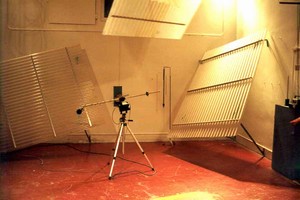 |
| Figure 12. Barrier absorption: Reverberation Room Method photo #2553 |
The amount of incident sound that a barrier transmits can be described by its sound Transmission Loss (TL). Measurements to determine a barrier's TL should be made in accordance with ASTM Recommended Practice E413-87.ref.16 TL is determined as follows:

dB(A)
where: SPLs is the sound pressure level (see Section 3.1) on the source side of the barrier; and
SPLr is the sound pressure level on the receiver side of the barrier.
For highway noise barriers, any sound that is transmitted through the barrier can be effectively neglected since it will be at such a low level relative to the diffracted sound, i.e., the sound transmitted will typically be at least 20 dB(A) below that which is diffracted. That is, if a sound level of 100 dB(A) is incident upon a barrier and only 1 dB(A) is transmitted, i.e, 1 percent of the incident sound's energy, then a TL of 20 dB(A) is achieved.
As a rule of thumb, any material weighing 20 kg/m2 (4 lbs/ft2) or more has a transmission loss of at least 20 dB(A). Such material would be adequate for a noise reduction of at least 10 dB(A) due to diffraction. Note that a weight of 20 kg/m2 (4 lbs/ft2) can be attained by lighter and thicker, or heavier and thinner materials. The greater the density of the material, the thinner the material may be. TL also depends on the stiffness of the barrier material and frequency of the source.ref.18
In most cases, the maximum noise reduction that can be achieved by a barrier is 20 dB(A) for thin walls and 23 dB(A) for berms. Therefore, a material that has a TL of at least 25 dB(A) or greater is desired and would always be adequate for a noise barrier. The following table gives approximate TL values for some common materials, tested for typical A-weighted highway traffic frequency spectra. They may be used as a rough guide in acoustical design of noise barriers. For accurate values, consult material test reports by accredited laboratories.
| Material | Thickness mm (inches) |
Weight kg/m2 (lbs/ft2) |
Transmission Loss (dB(A)) |
|---|---|---|---|
| Concrete Block, 200mm x 200mm x 405 (8" x 8" x 16") light weight | 200mm (8") | 151 (31) | 34 |
| Dense Concrete | 100mm (4") | 244 (50) | 40 |
| Light Concrete | 150mm (6") | 244 (50) | 39 |
| Light Concrete | 100mm (4") | 161 (33) | 36 |
| Steel, 18 ga | 1.27mm (.0.050") | 10 (2.00) | 25 |
| Steel, 20 ga | 0.95mm (0.0375") | 7.3 (1.50) | 22 |
| Steel, 22 ga | 0.79mm (0.0312") | 6.1 (1.25) | 20 |
| Steel, 24 ga | 0.64mm (0.025") | 4.9 (1.00) | 18 |
| Aluminum, Sheet | 1.59mm (0.0625") | 4.4 (0.9) | 23 |
| Aluminum, Sheet | 3.18mm (0.125") | 8.8 (1.8) | 25 |
| Aluminum, Sheet | 6.35mm (0.25") | 17.1(3.5) | 27 |
| Wood, Fir | 12mm (O.5") | 8.3 (1.7) | 18 |
| Wood, Fir | 25mm (1.0") | 16.1(3.3) | 21 |
| Wood, Fir | 50mm (2.0") | 32.7 (6.7) | 24 |
| Plywood | 12mm (0.5") | 8.3 (1.7) | 20 |
| Plywood | 25mm (1.0") | 16.1 (3.3) | 23 |
| Glass, Safety | 3.18mm (0.125") | 7.8 (1.6) | 22 |
| Plexiglass | 6mm (0.25") | 7.3 (1.5) | 22 |
The above table assumes no openings or gaps in the barrier material. Some materials, such as wood, however, are prone to develop openings or gaps due to shrinkage, warping, splitting, or weathering. Treatments to reduce/eliminate noise leakage for wood barrier systems are discussed in Section 5.4.1. Noise leakage due to possible gaps in the horizontal joints between panels in a post and panel "stacked panel" barrier system (see Section 4.1.2.1) should also be given careful consideration. Finally, some barrier systems are designed with small openings at the base of the barrier to carry water, which would otherwise pond on one side of the barrier, through the barrier. Two important consideration associated with these openings are: (1) Ensure that the opening is small [the effect of a continuous gap of up to 20 cm (7.8 in) at the base of a noise barrier is usually within 1 dB(A)], ref.32 and (2) Ensure that proper protection in the form of grates or bars is provided to restrict entry by small animals (cats, small dogs, etc.). Drainage considerations are also discussed in Section 7.1.2 and 7.1.3.
It should be noted that there are other ratings used to express a material's sound transmission characteristics. One rating in common use is the Sound Transmission Class (STC). STC is a single-number rating derived by fitting a reference rating curve to the TL values measured for the one-third octave frequency bands between 125 Hz and 4000 Hz. The reference rating curve is fitted to the TL values such that the sum of deficiencies (TL values less than the reference rating curve), does not exceed 32 dB, and no single deficiency is greater than 8 dB. The STC value is the TL value of the reference contour at 500 Hz. The disadvantage to using the STC rating scheme is that it is designed to rate noise reductions in frequencies of normal speech and office areas, and not for the lower frequencies of highway traffic noise. For frequencies of traffic noise, the STC is typically 5 to 10 dB(A) greater than the TL and, thus, should only be used as rough guide.
This section describes the various acoustical considerations involved in actual noise barrier design. Non- acoustical design considerations will be discussed in Sections 4 to 13). The acoustical considerations include:
Barrier design goals and insertion loss(Section 3.5.1);
Barrier length (Section 3.5.2);
Wall versus berm (Section 3.5.3);
Reflective versus absorptive (Section 3.5.4);
Other miscellaneous design considerations (Section 3.5.5).
The first step in barrier design is to establish the design goals. Design goals may not be limited simply to noise reduction at receivers, but may also include other considerations of safety and maintenance as well. These other considerations are discussed later in Sections 4 through 13.
In this section, the acoustical design goals of noise reduction will be discussed. Acoustical design goals are usually referred to in terms of barrier Insertion Loss (IL). IL is defined as the sound level at a given receiver before the construction of a barrier minus the sound level at the same receiver after the construction of the barrier. The construction of a noise barrier usually results in a partial loss of soft-ground attenuation. This is due to the barrier forcing the sound to take a higher path relative to the ground plane. Therefore, barrier IL is the net effect of barrier diffraction, combined with this partial loss of soft-ground attenuation.
Typically, a 5-dB(A) IL can be expected for receivers whose line-of-sight to the roadway is just blocked by the barrier. A general rule-of-thumb is that each additional 1 m of barrier height above line-of-sight blockage will provide about 1.5 dB(A) of additional attenuation (see Figure 13).
Figure 13. Line-of-sight
Properly-designed noise barriers should attain an IL approaching 10 dB(A), which is equivalent to a perceived halving in loudness for the first row of homes directly behind the barrier. For those residents not directly behind the barrier, a noise reduction of 3 to 5 dB(A) can typically be provided, which is just slightly perceptible to the human ear. Table 4 shows the relationship between barrier IL and design feasibility.ref.1
| Barrier Insertion Loss | Design Feasibility | Reduction in Sound Energy | Relative Reduction in Loudness |
|---|---|---|---|
| 5 dB(A) | Simple | 68% | Readily perceptible |
| 10 dB(A) | Attainable | 90% | Half as loud |
| 15 dB(A) | Very difficult | 97% | One-third as loud |
| 20 dB(A) | Nearly impossible | 99% | One-fourth as loud |
Noise barriers should be tall enough and long enough so that only a small portion of sound diffracts around the edges. If a barrier is not long enough, degradations in barrier performance of up to 5 dB(A) less than the barrier's design noise reduction may be seen for those receivers near the barrier ends. A rule-of-thumb is that a barrier should be long enough such that the distance between a receiver and a barrier end is at least four times the perpendicular distance from the receiver to the barrier along a line drawn between the receiver and the roadway (see Figure 14). Another way of looking at this rule is that the angle subtended from the receiver to a barrier end should be at least 80 degrees, as measured from the perpendicular line from the receiver to the roadway.
Figure 14. Barrier length
Sometimes due to the community and roadway geometry, there is not enough available area to ensure a proper-length barrier. In those cases, highway barrier designers may decide to construct the barrier with the ends curved inward towards the community (see Figure 15).
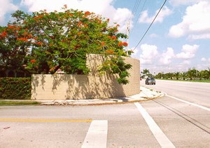
Figure 15. Barrier curved inward towards the community
photo #2617
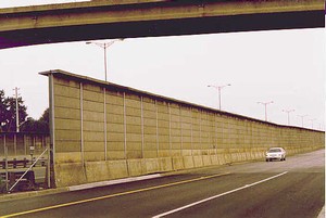
Highway noise barriers are typically characterized as a wall, a berm, or a combination of the two (see Figure 16). There are advantages and disadvantages to each type. The considerations that are examined in deciding whether to build a wall or a berm, include available area, materials, costs, aesthetics, and community concerns. Acoustically, for a given site geometry and comparable barrier height and length, a berm barrier will typically provide an extra 1 to 3 dB(A) of attenuation. Several factors contribute to this increase. First, the flat top of a berm diffracts the sound waves twice, resulting in a longer path-length difference, a larger Fresnel number, and, thus, more attenuation. Second, the surface of a berm is, essentially, grass-covered acoustically soft earth with side slopes closer to the sound path, which provides additional attenuation. However, because a berm is wider than a wall (thus, requiring more land than a wall when constructed) and because the 1 to 3 dB(A) additional attenuation is, at best, only barely perceptible to the human ear, a berm's acoustical advantage does not necessarily guarantee its choice versus a wall.
Figure 16. Wall, berm and combination noise barriers
A barrier without any added absorptive treatment is by default reflective (see also Section 3.4.1). A reflective barrier on one side of the roadway can result in some sound energy being reflected back across the roadway to receivers on the opposite side (see Figure 17).
It is a common phenomenon for residents to perceive a difference in sound after a barrier is installed on the opposite side of a roadway. Although theory indicates greater increases for a single reflection, practical highway measurements commonly show not greater than a 1 to 2 dB(A) increase in sound levels due to the sound reflected off the opposing barrier. While this increase may not be readily perceptible, residents on the opposite side of the roadway may perceive a change in the quality of the sound; the signature of the reflected sound may differ from that of the source due to a change in frequency content upon reflection.
Figure 17. Reflective noise paths due to a single barrier
Parallel barriers are two barriers which face each other on opposite sides of a roadway (see Figure 18). Sound reflected between reflective parallel barriers may cause degradations in each barrier's performance due to multiple reflections that diffract over the individual barriers. These degradations may be from 2 to as much as 6 dB(A) (see Figure 19).ref.19 That is, a single barrier with an insertion loss of 10 dB(A) may only realize an effective reduction of 4 to 8 dB(A) if another barrier is placed parallel to it on the opposite side of the highway. |
 |
| Figure 18. Parallel noise barriers photo #2968 |
Figure 19. Reflective noise paths due to a parallel barrier
The problems caused by both single and parallel barriers can be minimized using one or a combination of the following three methods:ref.19
For parallel barriers, ensure that the distance between the two barriers is at least 10 times their average height. A 10:1 width-to-height (w/h) ratio will result in an imperceptible degradation in performance. In recent studies, it was determined that as the w/h ratio increases, the insertion loss degradation decreases.ref.24 and ref.33 This decrease can be attributed to: (1) the decrease in the number of reflections between the barriers; and (2) the weakening of the reflections due to geometrical spreading and atmospheric absorption. Table 5 provides a guideline of three, general w/h ratio ranges and the corresponding barrier insertion-loss degradation (ΔIL) that can be expected.
| w/h Ratio | Maximum ΔIL in dB(A) | Recommendation |
|---|---|---|
| Less than 10:1 | 3 or greater | Action required to minimize degradation. |
| 10:1 to 20:1 | 0 to 3 | At most, degradation barely perceptible; no action required in most instances. |
| Greater than 20:1 | No measurable degradation | No action required. |
Apply sound absorptive material on either one or both barrier facades. See also Section 3.4.1. The decision to add a sound absorptive surface should be determined by weighing benefit versus cost. That is, what noise abatement benefits can be achieved for how many residents versus the costs of the application and maintenance of the absorptive treatments?
The answer is most important since the typical costs of noise absorptive material, whether integrated with the noise barrier at the time of barrier construction, or as a retrofit later on after the barrier is constructed, is usually $75 to $118/m2 ($7 to $11/ft2). Using an average cost of $97/m2 ($9/ft2) for example, for a 3.6-m (12 ft) high barrier, this would translate into an additional $0.4 million/km ($0.6 million/mi) in costs. ref.24 , ref.34 , ref.35 , ref.36 and ref.37
Tilt one or both of the barriers outward away from the road. Previous research has shown that an angle as small as 7 degrees is effective at minimizing degradations.ref.33 This solution, however, must consider locations higher than the opposite barrier because they may be adversely affected by the reflected sound.
Barriers which overlap each other (see Figure 20) are usually constructed to allow access gaps for maintenance, safety, and pedestrian purposes (see Section 9.4.1). A general rule-of-thumb is that the ratio between overlap distance and gap width should be at least 4:1 to ensure negligible degradation of barrier performance (see Figures 21). If a 4:1 ratio is not feasible, then consideration should be given to the application of absorptive material (see Section 3.4.1) on the barrier surfaces within the gap area.
Figure 20. Example of overlapping barriers photo #5902
Figure 21. Overlapping barriers
A barrier using concrete panels arranged in a "zig-zag-like" or "trapezoidal" configuration (see Section 4.1.2.3.1) is advantageous because it is structurally sound without the use of a foundation. This type of barrier can also be visually pleasing to motorists because it provides variation in form (see Figure 22). It does not, however, have any substantial additional sound attenuation benefits.
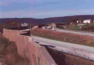
Figure 22. "Zig-zag" barrier photo #8057
There has been limited research into varying the shape of the top of a barrier (see Figure 23 and 24) for the purpose of shortening barrier heights and possibly attaining the attenuation characteristic of a taller barrier. The technical rationale is that additional attenuation can be attained by increasing the number of diffractions occurring at the top of the barrier. Shorter barrier heights could improve the aesthetic impact on communities and motorists by preserving more of the view.ref.18 and ref.38
Figure 23. Special acoustical considerations: tops of barriers
Studies have shown that a T-profile top barrier (see Figure 25) provides insertion losses comparable to a conventional top barrier when the difference in their heights is equal to the width of the T-profile top. When the two barriers are the same height, the T-profile top barrier has been shown to provide an additional 2.5 dB(A) insertion loss over the conventional top barrier. Y- and arrow-profile tops also performed better than conventional tops, however, to a lesser degree than the T- profile tops. ref.39 and ref.40 Cylindrical, pear-shape, curved, and Thnadner top barriers have not shown substantial benefits, unless an absorptive treatment was incorporated into the barrier tops.ref.41 and ref.42
 |
 |
| Figure 24. Special top of barrier photo #2395 |
Figure 25. T-profile top barrier photo #1312 |
Although there are some acoustical and aesthetic benefits associated with special barrier tops, the cost of constructing these shapes typically outweigh the cost of simply increasing the barrier's height to accomplish the same acoustic benefit.ref.43
|
Acoustical considerations for all noise barriers. |
||||
|---|---|---|---|---|
| Item# | Main Topic | Sub-Topic | Consideration | See Also Section |
| 3-1 | Atmospheric Effects | Atmospheric Absorption, Refraction, Turbulence | Field measurements should not be performed when wind speeds are greater than 5 m/s, or when strong winds with small vector components exist in the direction of propagation. | 3.3.1 14.1.2.1 15.1.2 |
| 3-2 | Barrier Design Goals | Barrier Sound Transmission | Barrier panel materials should weigh 20 kg/m2 or more for a transmission loss of at least 20 dB(A). | 3.4.2 |
| Barrier Length | Ensure barrier height and length are such that only a small portion of sound diffracts around the edges | 3.5.2 | ||
| Wall vs. Berm | A berm requires more surface area, but provides 1 to 3 dB(A) additional attenuation versus a wall. | 3.5.3 | ||
| Reflective vs. Absorptive | Communities may perceive sound level increases due to reflections. Sound reflected between parallel barriers may cause degradations in each barrier's performance from 2 to as much as 6 dB(A), but in most practical situations, the degradation is smaller. | 3.5.4 | ||
| Overlapping Barriers | Ensure the ratio between overlap distance and gap width (between barriers) is at least 4:1. | 3.5.5.1 | ||
| Special Tops for Barriers | The cost of constructing these special shapes typically outweigh the cost of simply increasing the barrier's height to accomplish the same acoustic benefit. | 3.5.5.3 |

