• Air Toxics
• CMAQ
• Conformity
• It All Adds Up

• Laws and Regulations
• Maps
• Policy and Guidance
• Research
  • General Practice
  • Air Quality Planning and SIPs
  • Emissions Analysis
  • Land Use
  • Multi-Jurisdictional (Complex) Areas
  • Project Level Conformity
  • Small Urban and Rural Areas
  • Tools & Methodologies
  • Transportation Control Measures
• Resources
• Models & Methodologies
• Training

FHWA → Environment → Air Quality → Conformity → Research → Improving Data

Improving Vehicle Fleet, Activity, and Emissions Data for On-Road Mobile Sources Emissions Inventories

4. Heavy-Duty Truck Activity Data

4.1. Background

Albeit a very small fraction in the total vehicle population, HDTs contribute disproportionately to the emissions inventory of on-road mobile sources. This is due to their high annual mileage and high emission rates. In addition, HDTs are also a significant source of idling emissions especially at truck stops and terminals as they often engage in long-duration idling activities (e.g., loading/unloading, heating/cooling the cabin during rest stops, etc.) at these locations [Miller et al., 2007; Frey et al., 2008]. Therefore, an accurate characterization of HDT activity is crucial to the construction of emissions inventory of on-road mobile sources.

In the current state of the practice, the HPMS has been used as a primary source for VMT data for various road and vehicle types, including HDTs [U.S. Environmental Protection Agency, 2005]. However, it does not include the information about traffic speed; and thus, the reported VMT cannot be characterized by speed bins. As vehicle emissions are sensitive to vehicle speed among other things, it is desirable to characterize VMT into multiple speed bins so that appropriate emission factors for each speed bin can be applied.

Alternatively, HDT activity can be estimated using travel demand models, especially those with a dedicated module for HDTs (e.g., [Southern California Association of Governments, 2008]). There has also been increasing interest in developing freight flow models (e.g., [Sarvareddy et al., 2005]), which can be used to derive truck trips and miles traveled. Nevertheless, these models are still in their early stages and have not been adopted widely. Also, the availability of measured truck traffic data, especially with regards to speed, that can be used for model validation is limited so that the accuracy of speed data from the models may be questionable.

Another method that has been used is to instrument a fleet of HDTs with GPS-based data loggers and log their travel activity over a period of time (e.g., [Battelle, 1999]). This method offers the most detailed and probably the most reliable information on HDT miles and speed. Also, it is able to capture the information about non-driving activities such as soak time and idling, which are not available in either the HPMS or travel demand models. However, this type of data collection requires significant resources; and thus, is usually performed for a small number of trucks and for a short period of time.

In this research, two alternative sources of HDT activity data including truck's electronic control unit (ECU) and telematics-based vehicle tracking and monitoring system were investigated to determine their potential for generating HDT activity data inputs for MOVES. In addition, a method was developed to fuse HDT activity datasets from multiple existing data sources to result in more refined and accurate HDT activity data.

4.2. Truck Electronic Control Unit Data

Modern diesel engines have rather sophisticated computers that control engine operation and allow manufacturers to program changes in efficiency and also allow for archiving of operating parameter information such as vehicle speed and engine speed. The original equipment manufacturers (OEMs) use this information to learn about typical vehicle operation as well as to monitor vehicle usage to determine if warranty repair service will be approved. A large number of variables are available on the engine downloads from electronically controlled engines a standard for the data links (SAE J1939) used in the heavy-duty vehicle industry was widely adopted by diesel engine manufacturers. The specific data available from the ECU varies by manufacturer, but generally includes engine identification and vehicle operational summaries as well as information on the current engine control program and the date when it was installed.

Heavy-duty diesel engines have been electronically controlled since the late 1980's. Part of the electronic control systems manages engine operation and another part collects and stores data on vehicle use. As the electronics have become more sophisticated they have enabled greater levels of control of engine operation (optimization of fuel use on extended cruises for example) as well as greater levels of data collection and storage. Modern electronic control systems collect and can provide operating information (temperatures, pressures, fuel consumption), customer programmable information (idle speed, cruise control mode), as well as diagnostic information. Engine manufacturers provide various specialized software systems for retrieving the data from these on-board computer systems using laptops or handheld computers. The specialized software and interface hardware are unique for each manufacturer.

While the different manufacturers record many of the same engine variables, the functions and the specific variables are not uniform across manufacturers. Even for the same manufacturers, different software versions also provide different amounts of data in different formats. Because of this lack of uniformity in variables, names, and data format, the task of compiling the data into a format useful for analysis is quite labor intensive.

A large number of variables are available on the engine downloads. The specific variables available vary from manufacturer to manufacturer, and across model years within manufacturers. For example, the Caterpillar Electronic Technician (CatET) software was used exclusively for the CAT vehicles. The ET program permits access to a range of diagnostic and archived engine and vehicle activity data. The engine variables available on a Caterpillar engine download are presented in Table 4-1. Similarly, Table 4-2 through Table 4-4 list the engine variables available on Cummins and Detroit Diesel downloads. Note that the fields in bold text are main headers.

Table 4-1. Variables available on downloads from Caterpillar engine

Cat Elec tronic Technician Cat ET2002A
Parameter	Parameter	Parameter
Vehicle ID	Idle Vehicle Speed Limit	Maintenance Indicator Mode
Engine Serial Number	Idle RPM Limit	PM1 Interval
ECM Serial Number	ldle/PTO RPM Ramp Rate	Engine Oil Capacity
Personality Module Part Number	ldle/PTO Bump RPM	Trip Parameters
Personality Module Release Date	Dedicated PTO Parameters	Fuel Correction Factor
Personality Module Code	PTO Configuration	Dash -Change Fuel Correction Factor
ECM Date/Time	PTO Top Engine Limit	Dash - PM1 Reset
Description	PTO Engine RPM Set Speed (0 - Off)	Dash - Fleet Trip Reset
Selected Engine Rating	PTO Engine RPM Set Speed A	Dash- State Selection
Rating Number	PTO Engine RPM Set Speed B	Theft Deterrent System Control
Rating Type	PTO to Set Speed	Theft Deterrent Password
Multi-Torque Ratio	PTO Cab Controls RPM Limit	Quick Stop Rate
Ad'.ertised Power	PTO Kickout Vehicle Speed Limit	Vehicle Actil.ity Report Parameters
Go\emed Speed	Torque Limit	Minimum Idle Time (0 = Off)
Rated Peak Torque	PTO Shutdown Time (0 - Off)	Dri\er Reward
Top Engine Speed Range	PTO Shutdown Timer Maximum RPM	Dri\er Reward Enable
Test Spec	PTO Activates Cooling Fan	Input Selections
Test Spec with BrakeSa\er	Engine/Gear Parameters	Fan 0\erride Switch
ECM Identification Parameters	Lower Gears Engine RPM Limit	Ignore Brake/Clutch Switch
Vehicle ID	Lower Gears Tum Off Speed	Torque Limit Switch
Engine Serial Number	Intermediate Gears Engine RPM Limit	Diagnostic Enable
ECM Serial Number	Intermediate Gears Tum Off Speed	Remote PTO Set Switch
Personality Module Part Number	Gear Down Protection RPM Limit	Remote PTO Resume Switch
Personality Module Release Date	Gear Down Protection Tum On Speed	PTO Engine RPM Set Speed Input A
Security Access Parameters	Top Engine Limit	PTO Engine RPM Set Speed Input B
Total Tattletale	Top Engine Limit with Droop	Starting Aid On/Off Switch
Last Tool to change Customer Parameters	Low Idle Engine RPM	Two Speed Axle Switch
Last Tool to change System Parameters	Transmission Style	Cruise Control On/Off Switch
ECM Wireless Communications Enable	Eaton Top 2 0\erride with Cruise Switch	Cruise Control Set!Resume/ Accei/Decel Switch
Vehicle Speed Parameters	Top Gear Ratio	Clutch Pedal Position Switch
Vehicle Speed Calibration	Top Gear Minus One Ratio	Retarder Off/Low/Med/High Switch
Vehicle Speed Limit	Top Gear Minus Two Ratio	Serl.ice Brake Pedal Position Switch #1
VSL Protection	Timer Parameters	Accelerator Pedal Position
Tachometer Calibration	Idle Shutdown Time (0 - Off)	Output Selections
Soft Vehicle Speed Limit	Idle Shutdown Timer Maximum RPM	Engine Running Output
Low Speed Range Axle Ratio	Allow Idle Shutdown 0\erride	Engine Shutdown Output
High Speed Range Axle Ratio	Minimum Idle Shutdown Outside Temp	Auxiliary Brake
Cruise Control Parameters	Maximum Idle Shutdown Outside Temp	Starting Aid Output
Low Cruise Control Speed Set Limit	A/C Switch Fan On-Time (0- Off)	Fan Control Type
High Cruise Control Speed Set Limit	Fan with Engine Retarder in High Mode	Passwords
Engine Retarder Mode	Engine Retarder Delay	Customer Password #1
Engine Retarder Minimum VSL Type	Smart Idle Parameters	Customer Password #2
Engine Retarder Minimum Vehicle Speed	Battery Monitor and Engine Control Voltage	Data Link Parameters
Auto Retarder in Cruise (0 - Off)	Engine Monitoring Parameters	Powertrain Data Link
Auto Retarder in Cruise Increment	Engine Monitoring Mode	System Parameters
Cruise/ldle/PTO Switch Configuration	Engine Monitoring Lamps	Personality Module Code
SoftCruise Control	Coolant Le\131 Sensor	FLS
Idle Parameters (Old PTO)	Maintenance Parameters	FTS

Table 4-2. Variables available on downloads from Cummins engine

Engine serial number	trip since last reset	other
ECM Image Name	distance	engine brake activations
signature/ISX-CM870	active service brake distance	engine protection shutdown overrides
CM870	cruise control distance	idle shutdowns
All trips (cumulative)	driver reward 1 distance	max imum accelerator vehicle speed fuel used
Distance	driver reward 2 distance	number of sudden decelerations
Total ECM distance	driver reward 3 distance	service brake actuations
total engine brake distance	driver reward 4 distance	trip averaQe engine speed
total engine distance	engine brake distance	trip average one gear down speed
total service brake distance	maximum accelerator vehicle speed distance	trip average top gear speed
fuel used	PTO drive distance	trip average vehicle speed
smart torque high torque fuel used	smart torque high torque distance	trip maximum engine speed
total cruise control fuel used	tri[l_ distance	trip maximum engine speed
total fuel used	trip_g_ear down distance	trip maximum vehicle speed
total gea down fuel used	trip percent distance vehicle overspeed 1	time
total idle fuel used	trip percent distance vehicle overspeed 2	cruise control time
total loaded PTO drive fuel used	trip top gear distance	driver rewa rd 1 time
total maximum accelerator vehicle SQSed fuel used	vehicle overspeed 1 distance	driver reward 2 time
total PTO drive fuel used	vehicle overspeed 2 distance	driver reward 3 time
total PTO fuel used	fuel used	driver reward 4 time
total top gear fuel used	cruise control fuel used	engine brake time
multiple PTO	driver reward 1 fuel used	engine brakes
PTO device 1	driver reward 2 fuel used	fan on time
PTO device 2	driver reward 3 fuel used	fan time air conditioning pressure switch
PTO device 3	driver reward 4 fuel used	fan time due to engine conditions
PTO device 4	maximum accelerator vehicle speed fuel used	fan time fan control switch
PTO device 5	PTO drive fuel used	fan time with vehicle speed
PTO device 6	PTO fuel used	fan time without vehicle speed
PTO device 7	smart torque high torque fuel used	maximum accelerator vehicle speed time
PTO device 8	trip average fuel economy	! percent time at idle
fuel	trip average fuel rate	percent time in cruise control
PTO device 1 total fuel used	trip drive average fuel economy	percent time in PTO
PTO device 2 total fuel used	trip drive fuel used	! percent time in top gear
PTO device 3 total fuel used	trip fuel used	percent time one gear down
PTO device 4 total fuel used	trip gear down fuel used	PTO drive time
PTO device 5 total fuel used	trip idle fuel used	PTO time
PTO device 6 total fuel used	trip top gear fuel used	smart torque high torque time
PTO device 7 total fuel used	vehicle overspeed 1 fuel used	trip gear down time
PTO device 8 total fuel used	vehicle overspeed 2 fuel used	trip idle time
time	multiple PTO	trip percent distance in cruise control
PTO device 1 total time	PTO device 1	trip percent distance in top gear
PTO device 2 total time	PTO device 2	trip percent distance one gear down
PTO device 3 total time	PTO device 3	trip percent fan on time
PTO device 4 total time	PTO device 4	trip percent fan on time due to air conditioning pressure switch
PTO device 5 total time	PTO device 5
PTO device 6 total time	PTO device 6	trip percent fan on time due to engine conditions
PTO device 7 total time	PTO device 7	trip percent fan on time due tofan control switch
PTO device 8 total time	PTO device 8	trip percent fan on time with vehicle speed
other	fuel	trip percent fann on time without vehicl speed
total average engine speed	PTO device 1 trip fuel used	trip_ service brake time
total average fuel economy	PTO device 2 trip fuel used	trip time
total engine brake activations	PTO device 3 trip fuel used	trip top gear time
total engine protection shutdown manual overrides	PTO device 4 trip fuel used	vehicle overspeed 1 time
time	PTO device 5 trip fuel used	vehicle overspeed 2 time
smart torque high torque time	PTO device 6 trip fuel used
total cruise control time	PTO device 7 trip fuel used
total ECM time (key on time)	PTO device 8 trip fuel used
total engine brake time	time
total engine run time	PTO device 1 trip time
total gear down time	PTO device 2 trip time
tota l idle time	PTO device 3 trip time
total maximum accelerator vehicle speed time	PTO device 4 trip time
total PTO drive time	PTO device 5 trip time
total PTO time	PTO device 6 trip time
total service brake time	PTO device 7 trip time
total top gear time	PTO device 8 trip time

Table 4-3. Variables available on downloads from Detroit Diesel engine (summary version)

Vehicle Unit Number	engine brake totals	VSG totals
Engine serial Number	time	fuel
ECU version	I percentages	time
Engine totals	on idle	o_l)_timized idle totals
Accumulated totals	on cruise	optimized idle not enabled
fuel	last de-green reset	cruise totals
time	distance	time
distance	trip totals	engine brake totals
idle totals	accumulated totals	time
fuel	fuel	fuel econom_y_
time	time	percentages
VSG totals	distance	on idle
fuel	idle totals	on cruise
time	fuel
optimized idle totals	time
cruise totals
time

Table 4-4. Variables available on downloads from Detroit Diesel engine (detailed version)

print date	speeding A(>=66 mph and <71 mph)	optimized idle batter charging run time
trip	count	normal slats
vehicle id	time	continuous run starts
driver id	percent	alternate battery time starts
odometer	speeding B (>=71 mph)	fan on time
trip distance	count	total time
trip fuel	time	engine system
fuel economy	percent	manual
avg drive load	highest speed occurred	AIC
avg vehicle speed	coasting time	pump on time
driving time	coasting percent	time
driving percent	trip time	distance
driving fuel	fuel consumption	fuel
driving economy	idle time	eQgine utilization
vehicle speed limiting	idle percent	vehicle utilization
time	idle fuel	hard brake limit
Ipercent	VSG (PTO) time	stop idle limit
distance	VSG (PTO) percent	top gear limit
fuel	VSG (PTO) fuel	top gear-1 limit
top gear	stop idle time	ECM S/W
time	stop idle percent	ECM type
percent	stop idle fuel	config. Change
distance	over rev limit	idle method
fuel	count	idle-load method
top gear -1	time	idle-RPM limit
time	percent	reset lockout
percent	highest rpm occurred	fleet time zone
distance	diag. records	maintenance visual reminder
fuel	hard brake count	enabled
cruise	brake count	percentage
time	eng. Brake time	vehicle speed bands (mph)
percent	optimized idle time	engine speed bands (rpm)
distance	active	percent load bands(%)
fuel	run	trip status
top gear cruise	battery
time	engine temp.
percent	thermostat
distance	extended idle
fuel	continuous

4.2.1. Example Dataset

Summary data from an ECU can be downloaded using engine manufacturer specific diagnostic software such as Cat ET for Caterpillar, Detroit Diagnostic Link for Detroit Diesel, and INSITE for Cummins. The cost for the software and the hardware required to connect to the on-board ECM is in the range of $1,000-$3,000 depending on manufacturer. Data available on ECU downloads also vary by manufacturer and software version. With the proper knowledge and skill on how to use the software and hardware, each ECU download takes approximately 10 to 15 minutes. It can be seen that the task of downloading ECM data from trucks is simple and does not require a significant amount of resources. What is more difficult is a time and resource burden in acquiring trucks for the download.

Alternatively, there are many truck repair shops that perform ECU diagnostic as part of their everyday job. These shops vary in size (in terms of the average number of trucks they work on each day) and capability (some shops only use basic code readers, which do not have access to the ECU summary data). Although many shops have the proper diagnostic software, it is not common practice to download the ECU summary data and store it. Downloading the ECU summary data is often done only upon customers' request, and the downloaded data is not typically stored by the shops except for some authorized dealer shops that handle warranty repairs. In these instances, the ECU summary data is sent to a corporate database.

Still, it is possible to contract with truck repair shops or truck fleets that have proper software and deal with a large volume of trucks to collect a sizable amount of ECU summary downloads in a timely manner. In this study, a small sample of 150 ECU downloads were obtained through working with truck fleets in the state of New York. This area was chosen because it is under nonattainment and has major seaports that process a significant portion of U.S. freight flow (see Figure 4-1).

The acquired ECU downloads are from four engine manufactures:

• Caterpillar - 2 downloads
• Cummins - 55 downloads
• Detroit Diesel - 16 downloads
• Hino - 77 downloads

Figure 4-2 presents the model year distribution of HDTs in the ECU download sample by engine manufacturer. It is shown that most of the HDTs with known model year are less than five years old (note that the ECU downloads were acquired in 2010).

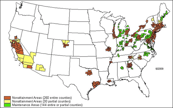
Sources: http://www.epa.gov/air/oaqps/greenbk/map8hrnm.html

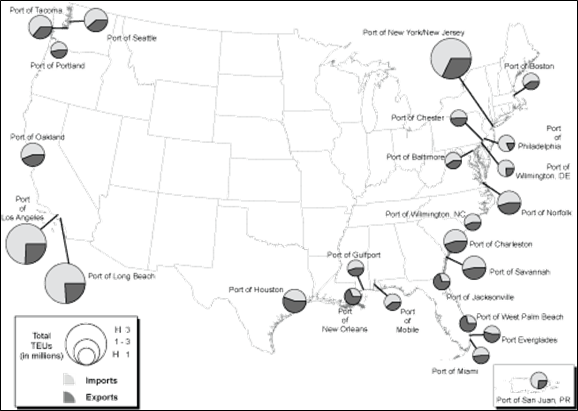
Source: http://www.bts.gov/publications/americas_container_ports/2009/html/figure_08.html

Figure 4-1. (top) 8-hr ozone nonattainment and maintenance areas in the U.S., and

(bottom) 2008 freight flow at U.S. ports

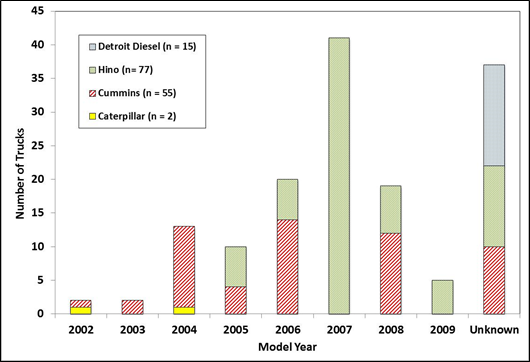
Figure 4-2. Model year of HDTs in the ECU download sample.

4.2.2. Data Processing and Analysis

ECU downloads are usually generated as a customized report and not in a file format that can be readily transferred to a database. The ECU downloads obtained in this study were provided in a PDF format. For each engine manufacture format, the data items of interest were identified and manually entered into an Excel spreadsheet. For creating HDT activity data inputs for MOVES, the key data items of interest include:

• Total distance
• Total hours
• Time at idle
• Time at power take-off (PTO)

Based on these data items, additional information were calculated as follows:

Note that is PTO is a splined driveshaft, usually on a tractor or truck, that can be used to provide power to an attachment or separate machine. The PTO allows implements to draw energy from the tractor's engine, which increases emissions.

4.2.3. Results and Discussion

Figure 4-3 shows the distributions of the average speed of all HDTs in the sample. When idling is included, the mid speed range of 35-40 mph dominate the distribution. When idling is not included in the calculation, the typical "driving" speed of these HDTs is around 45-55 mph. These trends are similar to those found in a similar study using ECU downloads from HDTs in California [Boriboonsomsin et al., 2010].

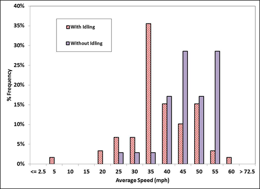
Figure 4-3. Distributions of average speed with and without idling.

Figure 4-4 presents the distributions of idling and PTO activity. According to the figure, the percentage that the HDTs are in idle mode is distributed across a wide range of 2.5-45% with some outliers at 55% and more. In general, these HDTs idle for about a quarter of the total operating hours, which is considered significant. On the other hand, over 60% of the HDTs in this sample rarely use PTO by more than 10%. When compared with the trends from the California study [Boriboonsomsin et al., 2010], it is found that the HDTs in this study spend a smaller fraction of their operating time in idle and PTO modes.

It should be noted that the idling time in ECU downloads cannot be differentiated between regular idling and extended idling, which is a new data inputs in MOVES. It is characterized by a higher engine speed, and thus higher emissions. However, the information regarding the total idling time can be combined with the information of extended idling from specialized studies (e.g., [Frey et al., 2008]) to estimate the total extended idling hours.

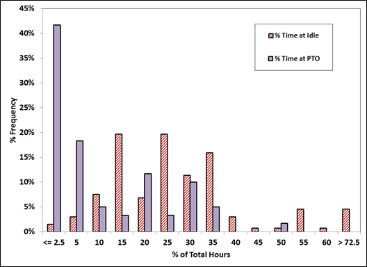
Figure 4-4. Distributions of percent time at idle and at PTO.

4.3. Truck Telematics Data

For the last couple of years, the use of wireless communication or telematics technology has been increasingly adopted by the fleet management industry. There is now a large number of fleet vehicles that are equipped with telematics-based vehicle tracking and monitoring systems which can wirelessly transmit the position information of the vehicles that is obtained from an on-board GPS device to a system server on a periodic basis. Furthermore, some systems are also connected to the vehicle's on-board diagnostic bus (OBD-II for light-duty vehicles and SAE J1939 bus for heavy-duty trucks), allowing not only the vehicle's position but also vehicle and engine operating conditions (e.g., engine speed, fuel use, etc.) to be monitored and reported in real-time (e.g., [NetworkFleet, 2011]).

These vehicle tracking and monitoring systems have potential to be a very rich source of HDT activity data. However, they have not been fully evaluated, especially in the context of supporting emissions inventory development. The objectives of this subtask in this research are: 1) to examine how telematics data from HDT tracking and monitoring systems can be used to generate HDT activity data inputs for the MOVES model; and 2) to assess the advantages and limitations of this data source.

4.3.1. Example Dataset

The HDT telematics data used in this study are from the Highway Visibility System (HIVIS) [Calmar Telematics, 2011]. HIVIS is a private database containing several hundred million records of commercial vehicle activity data from the telematics-based tracking and monitoring systems in the vehicles of participating fleets. Each of the participating fleets has arranged for the telematics data from their fleet operations to be automatically transmitted to HIVIS in exchange of both monetary compensation and access to the database for their own use. The HIVIS database has been used in a number of ways such as measuring truck travel time, developing truck trip tables, and studying truck VMT fees. At the time of reporting, it has never been used in air quality-related studies.

The HIVIS dataset used in this study comes from a collective fleet of more than 2,000 Class 8 HDTs traveling across the U.S. for the entire year of 2010. These HDTs comprise a broad cross-section of the commercial vehicle industry. Within the database there are single- and multi-trailers, dry bulk trailers, petroleum tankers, and milk trucks. In general, there is approximately a 90/10 split between combination trucks and straight trucks.

Figure 4-5 shows the plot of 1,791,816 GPS points from the HIVIS dataset across the U.S. in January 2010. A majority of the data points is clustered around the Northeast and Southern California regions where the home bases of most of the trucks in the dataset are located. It should be noted that these two regions are home of the three major ports that carry a significant portion of U.S. freight flow. Specifically, the ports of Los Angeles, Long Beach, and New York/New Jersey together carried about 50% of the total U.S. import and export containers in 2009 [Port Import Export Reporting Service, 2011].

It can be seen from the pattern of the GPS points in Figure 4-5 that many of the trucks are operated in large regional or long-haul fleets while some are operated locally within metro areas. Table 4-5 lists the top 20 metropolitan planning organization (MPO) areas that have the highest number of data points in this dataset. As expected, most of them are in the northeastern states, especially New York, as well as in California.

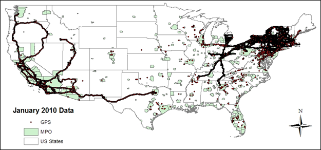
Figure4-5. U.S. nationwide truck telematics data for January 2010.

Table 4-5. Top 20 MPOs with the most number of data points in January 2010 dataset

No.	Metropolitan Planning Organization	State	Population in Year 2000	No. of Data Points
1	Capital District Transportation Committee	NY	780,467	513,270
2	Greater Buffalo-Niagara Regional Transportation Council	NY	1,170,111	228,240
3	San Diego Association of Governments	CA	2,813,833	214,097
4	Southern California Association of Governments	CA	16,516,006	100,543
5	Herkimer-Oneida Counties Transportation Study	NY	299,896	99,712
6	Adirondack/Glens Falls Transportation Council	NY	138,171	75,041
7	Syracuse Metropolitan Transportation Council	NY	468,018	67,285
8	Binghamton Metropolitan Transportation Study	NY	215,457	58,637
9	Berkshire MPO	MA	134,953	54,469
10	Central Massachusetts MPO	MA	518,480	42,569
11	Pioneer Valley MPO	MA	608,479	40,675
12	Lackawanna-Luzerne Transportation Study	PA	532,545	32,325
13	Orange County Transportation Council	NY	341,367	31,873
14	Genesee Transportation Council	NY	823,147	29,119
15	North Jersey Transportation Planning Authority	NJ	6,310,989	25,194
16	Ulster County Transportation Council	NY	177,749	23,758
17	Chittenden County MPO	VT	146,571	22,359
18	Capital Region COG	CT	721,320	16,742
19	Southeast Michigan COG	MI	4,833,493	11,840
20	New York Metropolitan Transportation Council	NY	12,068,148	11,158

The particular data items that are collected from the trucks vary with the particular telematics solution that each fleet uses. Some fleets use simple tracking systems which merely return the vehicle's location at regular periods of time. Other fleets opt for highly sophisticated systems which also access the vehicle's data bus and can potentially return hundreds of vehicle and engine operating variables such as fuel consumption, engine speed, coolant temperature, and braking events.

The HIVIS dataset obtained in this study consist of two data files - a Trip Summary file and a Trip Points file. The Trip Summary file contains aggregated trip information while the Trip Points file contains the information regarding individual telematics data points. Table 4-6 lists the data items in each file and their description. Note that some data items such as tractorYear, engineMake, Distance, FuelConsumed, and ptRPM are only available for a limited number of trucks depending on the particular telematics solution used by the fleet as discussed above.

Note that the data in the Trip Points file are similar to what can be obtained from instrumented vehicle studies. The main difference is that instrumented vehicle studies usually record data at a one-second interval while the data in the Trip Points file are much coarser (e.g, 30-second or 5-minute reporting interval depending on the fleet). This is because fleets have to balance the resolution of the data they obtain against the cost of the wireless transmission of the data. Generally, that level of data resolution is sufficient for the purpose of tracking and monitoring their vehicles.

Table 4-6. Data items and their description

Data Items	Description
Trip Summary File
tripNum	Unique identifier for this trip within this set of dated files
Veh_ID	Unique identifier for the vehicle, which is randomized weekly
tractorYear	Year of the tractor
tractorMake	Make of the tractor
tractorModel	Model of the tractor
engineMake	Make of the engine
engineModel	Model of the engine
odometerRange	The engines odometer range, truncated to 10,000 miles
HIVIScommodityCode	Commodity Code Abbreviation for the vehicle's fleet within HIVIS
DataMonth	Month that this trip occurred (GMT)
DataDOW	Day of week that this trip occurred (GMT)
firstLocTime5min	Time of day that this trip started (GMT), truncated to a 5-minute interval
lastLocTime5min	Time of day that this trip ended (GMT), truncated to a 5-minute interval
elapsedMinutes	Number of minutes elapsed during this trip
numPts	Number of data point locations recorded during this trip
pctSpeedBin0	Percent of data points with speed of 0mph
pctSpeedBin1	Percent of data points with speed < 2.5mph
pctSpeedBin2	Percent of data points with speed >= 2.5mph and < 7.5mph
pctSpeedBin3	Percent of data points with speed >= 7.5mph and < 12.5mph
pctSpeedBin4	Percent of data points with speed >= 12.5mph and < 17.5mph
pctSpeedBin5	Percent of data points with speed >= 17.5mph and < 22.5mph
pctSpeedBin6	Percent of data points with speed >= 22.5mph and < 27.5mph
pctSpeedBin7	Percent of data points with speed >= 27.5mph and < 32.5mph
pctSpeedBin8	Percent of data points with speed >= 32.5mph and < 37.5mph
pctSpeedBin9	Percent of data points with speed >= 37.5mph and < 42.5mph
pctSpeedBin10	Percent of data points with speed >= 42.5mph and < 47.5mph
pctSpeedBin11	Percent of data points with speed >= 47.5mph and < 52.5mph
pctSpeedBin12	Percent of data points with speed >= 52.5mph and < 57.5mph
pctSpeedBin13	Percent of data points with speed >= 57.5mph and < 62.5mph
pctSpeedBin14	Percent of data points with speed >= 62.5mph and < 67.5mph
pctSpeedBin15	Percent of data points with speed >= 67.5mph and < 72.5mph
pctSpeedBin16	Percent of data points with speed >= 72.5mph
Distance	Approximate distance traveled, in miles, during this trip
FuelConsumed	Approximate amount of fuel consumed, in gallons, during this trip
CalculatedFuelEfficiency	Approximate fuel economy, in miles per gallon, during this trip
Trip Points File
tripNum	Unique identifier for this trip within this set of dated files
ptOrder	This point’s order within the trip
Latitude	This point’s locational latitude
Longitude	This point’s locational longitude
Speed	This point’s speed (from engine data bus if available, otherwise from GPS)
Direction	This point’s GPS direction
elapsedSeconds	Number of seconds elapsed since beginning of trip
ptDistance	Travel distance since last point
ptFuel	Fuel level, in percentage
ptRPM	Engine speed, in revolutions per minute

4.3.2. Data Processing and Analysis

The data analysis methodology generally involves multiple steps, which are different for different MOVES data inputs. Described below are selected data analysis steps that are nontrivial as compared to other steps.

Map Matching

Map matching is the assignment of each data point to a geographic entity based on its position in relative to surrounding geographic entities, for example, assigning a data point to one road link or one MPO area. This is a critical analysis step for characterizing HDT activity into one of the five road types in MOVES, which are off-network, urban restricted, urban unrestricted, rural restricted, and rural unrestricted. It was performed using geographic information system (GIS) software.

To perform map matching of data points for road type characterization in GIS, a digital road network with road type information in shapefile format is required. In this study, three publicly available digital road network shapefiles including HPMS, TIGER/Line 2000, and ESRI StreetMap USA were examined. The ESRI StreetMap USA was selected because it has better quality than the HPMS and is more up-to-date than the TIGER/Line 2000. The road type attribute called "CLASS_RTE" ranges from 0 to 9. According to their definition (not shown here for brevity), the types 0-2 and 7 are considered restricted access and the rest unrestricted access. The point-to-line matching algorithm was used where a data point is assigned to a road link that has the shortest orthogonal distance to the data point. To differentiate between urban and rural areas, an urban boundary shapefile was used where a data point is considered to be on an urban road if it is within the boundary of an urban area. Since the data points are across the entire U.S., another round of map matching was also performed to differentiate the data points by time zone before calculating local time from the reported Greenwich Mean Time (GMT).

Off-Network Activity

The MOVES model allows users to input off-network activity, which is the portion of activity that is not reflected in the other four road types. Examples are driving on an unspecified road or idling in a parking lot. In this study, off-network activity is represented by data points that are not on one of the road links in the ESRI StreetMap USA network. Since the road network shapefile is a polyline feature (i.e., a road is represented by only its centerline and not its width), a criterion must be established to determine whether a data point is on road or off road. Figure 4-6 shows the percentage frequency distribution of the orthogonal distance from GPS point to road centerline. By considering this figure, along with the typical GPS horizontal positioning accuracy (30 ft) and lane width of roadways (10-12 ft), the criterion was set that the GPS points having the orthogonal distance from road centerline greater than 60 feet are considered to be off network. Based on this criterion, approximately 15% of the GPS points are off network.

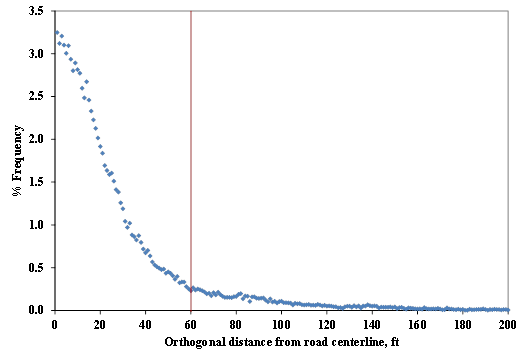
Figure 4-6. Orthogonal distance of GPS points from road centerline.

Road Centerline Distance Calculation

As mentioned earlier, some fleets in the HIVIS do not report distance values as their telematics systems are not connected to the vehicle's odometer. For these fleets, the distance between two consecutive GPS points needs to be calculated based on their GPS coordinates (i.e., latitude and longitude). However, this cannot be calculated as a Euclidean distance because its value may be lower than the actual travel distance along the roads, especially at curves or intersections. In addition, the data interval is large enough to cause two consecutive GPS points to be in different areas. In this study, the road centerline distance between two consecutive GPS points was calculated by first projecting each point onto the road centerlines and then calculating the distance using a shortest-path algorithm.

4.3.3. Results and Discussion

Several HDT activity data inputs for MOVES were derived from the HIVIS dataset. This section presents some of the resulting data inputs for January 2010 (representing winter). Where applicable, the data inputs for July 2010 (representing summer) as well as the default values in MOVES2010 are also given. A complete set of MOVES data inputs that were derived is provided in Appendix D.

VMT Fraction by Road Type

RoadTypeVMTFraction is the fraction of total VMT for each vehicle type (i.e., source type in MOVES) on each of the five road types. For MOVES2010, this fraction is derived from the 1999 Federal Highway Administration (FHWA) Highway Statistics, Tables VM-1 and VM-2 [U.S. Environmental Protection Agency, 2010]. Table 4-7 presents such fractions as well as the ones derived in this study. The off-network VMT for the base year 1999 in MOVES2010 is zero because the reported VMT in the FHWA Highway Statistics are assumed to include all VMT. In this study, off-network VMT were also not calculated as road centerline distance cannot be calculated for the GPS points that are considered to be off network. The total VMT on the other four road types are 2,966,869 miles for January 2010 and 5,662,240 miles for July 2010.

According to Table 4-7, it is observed that the fraction for January 2010 derived in this study is similar to that in MOVES2010. However, the one for July 2010 is very different where the greatest fraction of VMT occurred on urban unrestricted roads. This difference may be due to the difference in fleet composition in the HIVIS dataset for the two months. As HIVIS collects telematics data from multiple fleets, HDTs from any fleets may be removed from HIVIS (for service or other reasons) anytime. In addition, new fleets may be added to HIVIS anytime as well. Thus, the distinct RoadTypeVMTFraction for July 2010 seems to be caused by urban delivery fleets being added to HIVIS prior to that month.

Table 4-7. RoadTypeVMTFraction.

RoadType ID	Description	This Study		MOVES2010
		January 2010	July 2010	1999
1	Off-Network	-	-	-
2	Rural Restricted	0.3350	0.2373	0.3247
3	Rural Unrestricted	0.3047	0.2898	0.2941
4	Urban Restricted	0.1869	0.1555	0.2075
5	Urban Unrestricted	0.1734	0.3174	0.1737
	Total	1.0000	1.0000	1.0000

VMT Fraction by Weekday/Weekend and by Hour

MOVES uses VMT fraction by month, day, and hour to estimate emissions for every hour of every day of the year. In MOVES2010, these temporal distributions of VMT are derived from a 1995 data sample of 5,000 continuous traffic counters distributed throughout the U.S., which was used in a report by the Office of Highway Information Management [Festin, 1996]. The data sample is not differentiated by month or vehicle type. Thus, the same temporal VMT distributions are used for every month and source type in MOVES2010 [U.S. Environmental Protection Agency, 2010]. However, it is very likely that these distributions are biased towards passenger cars as they account for the majority of the vehicles in the data sample.

Table 4-8 provides the default DayVMTFraction in MOVES2010 and the ones derived in this study. It is observed that the VMT in this study are generally 10% higher on weekdays (and thus, 10% lower on weekends) than what MOVES2010 indicates. For instance, it is found that 86% of the VMT on urban roads in January 2010 occurred on weekdays while only 76% did so according to the default DayVMTFraction fraction in MOVES2010. This is true for both rural and urban roads, and for both January and July 2010. This trend is likely because HDTs do not accumulate miles from social and recreational travel on weekends as passenger vehicles do.

Table 4-8. Day VMTFraction.

Day	This Study				MOVES2010
	January 2010		July 2010		1995
	Rural	Urban	Rural	Urban	Rural	Urban
Weekday	0.8207	0.8594	0.7967	0.8621	0.7212	0.7624
Weekend	0.1793	0.1406	0.2033	0.1379	0.2788	0.2376
Total	1.0000	1.0000	1.0000	1.0000	1.0000	1.0000

Figure 4-7 shows the diurnal profiles of the daily VMT (i.e., HourVMTFraction) by road type for January 2010. They have a totally different shape from the typical two-peak profile of commute traffic. For the HDTs in this study, they drove quite a large portion of their miles during nighttime (8 p.m. - 6 a.m.) and their VMT was highest around midday (11 a.m. - 12 p.m.). This pattern is consistent with the one found in another study based on ECM data [Boriboonsomsin et al., 2010]. By comparing between the two road types, it is observed that there was a higher portion of VMT on rural roads in the evening and late night than in the early morning. This is opposite for urban roads.

Figure4-7. HourVMTFraction.

Average Speed Distribution

AvgSpeedDistribution is the fraction of driving time for each source type, road type, day, and hour in each average speed bin. There are 16 speed bins in MOVES, with the average speed value of 2.5 (speed < 2.5 mph), 5 (2.5 mph <= speed < 7.5 mph), 10 (7.5 mph <= speed < 12.5 mph), 70, (67.5 mph <= speed < 72.5 mph), and 75 (72.5 mph <= speed) [U.S. Environmental Protection Agency, 2010]. In MOVES2010, the average speed distributions for urban roads are derived from the default VMT-speed distributions in MOBILE6 [Systems Applications International, Inc., 2001], which do not vary by vehicle type. The average speed distributions for rural roads are derived from instrumented vehicle studies of light-duty vehicles (LDVs) collected in California [Sierra Research, Inc., 2004]. It has been shown that the speed distribution of HDTs is likely to be different from that of LDVs, especially in states or areas where the two vehicle types are imposed by different speed limits [Boriboonsomsin et al., 2011].

Figure 4-8. AvgSpeedDistribution, urban restricted roads, weekday, January 2010

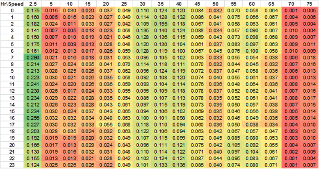
Figure 4-9. AvgSpeedDistribution, urban unrestricted roads, weekday, January 2010

Figure 4-8 and Figure 4-9 show the AvgSpeedDistribution for urban restricted roads and urban unrestricted roads on weekdays derived from the January 2010 dataset. The fraction is color coded from red (low value) to green (high value). Based on the patterns of the color code, the following observations are made:

• For urban restricted roads, the HDTs spent most of their time at free-flow speeds around 60-65 mph. This is consistent with the finding in [Boriboonsomsin et al., 2011]. Also, there was a fair amount of time spent in the 2.5-mph speed bin, which is probably not due to congestion but rather a result of idling on roadsides or rest stops.
• For urban unrestricted roads, the HDTs spent the largest fraction of their time each hour in the 2.5-mph speed bin, probably idling at traffic lights or loading/unloading zones. The most dominant non-idle speed range is 30-40 mph, which is consistent with the typical speed limits found on that type of road. Note that the small fraction of time at very high speeds (70-75 mph) shown in the figure is very unlikely in the real world, and probably is caused by errors from the map matching.

Trip Start Locations and Distributions

Data regarding the number of trip starts (or vehicle starts) by area and by time of day are necessary for estimating start emissions. In MOVES2010, StartAllocFactor is the fraction that distributes the nationwide estimates of the number of trip starts to individual counties. There is no available data on the number of trip starts by county at a national level, so VMT by county obtained from the National Mobile Inventory Model database is used as a surrogate to determine this fraction [U.S. Environmental Protection Agency, 2010].

Figure 4-10 shows the number of trip starts by county derived from the January 2010 dataset in this study. The data pattern is similar to the one in Figure 4-5, and reflects the fact that many of the trucks in this dataset are operated out of the Northeast and Southern California regions. Although the truck samples in the dataset are biased towards these two regions, a weighting function such as one based on VMT by county as used in MOVES2010 could allow the number of trip starts in these two regions to be projected to counties in the other regions. However, this is out of the scope of the current study.

In addition to the spatial allocation factor, MOVES also uses trip starts distributions by time of day to allocate the number of trip starts temporally. Figure 4-11 shows trip starts distributions by time of day for both weekday and weekend derived from the January 2010 dataset in this study. According to the figure, the trip starts distributions of both day types have a similar shape with the peak occurring in the morning (9-10 a.m.). For both weekdays and weekends, a majority of the trip starts occurred during daytime, but there were more trip starts during nighttime on weekends as compared to weekdays.

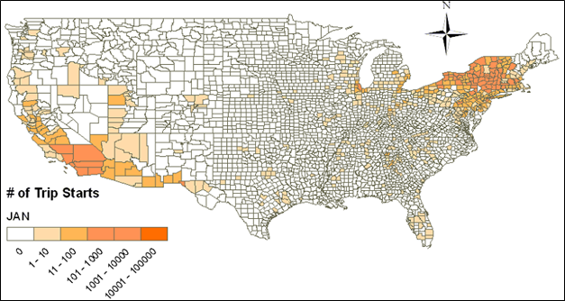
Figure 4-10. StartAllocFactor, January 2010.

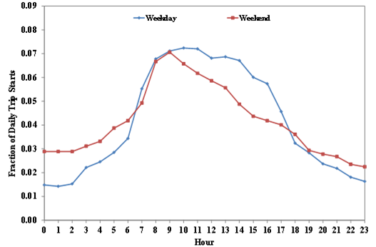
Figure 4-11. Trip starts distribution by time of day, January 2010.

4.4. Truck Activity Data Fusion

In the previous sections, new sources of HDT activity data are presented and methods for using them to generate HDT activity data inputs for MOVES are described. In this section, the focus is turned to the fusion of data from existing sources to improve HDT activity data inputs for MOVES.

Each of the existing HDT activity data sources provides different unique data elements but also lacks one or more other data elements. For instance, the Highway Performance Monitoring System (HPMS) can provide estimates of truck miles traveled by roadway functional class but it provides no information on the speed at which those truck miles are traveled or how much weight is carried by the trucks on those miles. On the other hand, weigh-in-motion (WIM) stations can provide the information regarding truck speed and loaded truck weight but only at a limited number of locations. For example, California has only 106 WIM stations throughout the entire state. In contrast, it has more than 8,100 vehicle detector stations (VDS), each comprised of multiple single-loop detectors, across its freeway systems. Figure 4-12 shows the comparison between the coverage of WIM stations and VDS in the Los Angeles area.

Efforts have been made in fusing data from different sources to create better HDT activity data inputs. For example, statistical models were developed based on truck traffic speed from a WIM station and overall traffic speed from a nearby VDS so that truck traffic speed at other VDS can be estimated based on the knowledge of the overall traffic speed alone [Boriboonsomsin et al., 2011]. According to that research, it was found that the regional truck activity in terms of VMT by speed distribution on Southern California freeways was significantly different from the activity of the overall traffic. The resulting emission inventories showed that using the HDT-specific speed distribution rather the overall speed distribution reduced the estimates of NO_x emissions by 4% and PM_2.5 emissions by 26%.

In MOVES, the basis of vehicle activity for exhaust running emissions is source hours operating (SHO) rather than VMT. SHO is characterized by vehicle operating mode (OpMode) bins, which is a function of vehicle specific power (VSP) and speed, rather than speed bins. To add to that complexity, VSP is a function of speed, acceleration, mass, road grade (if any), and vehicle-specific coefficients (i.e., rolling, rotating, and drag coefficients). Therefore, it can be seen that developing vehicle activity data inputs for MOVES is not a trivial task. Recognizing this challenge, the U.S. EPA has developed tools and methodologies that simplify the processes of developing vehicle activity data inputs for MOVES. These methodologies are based on a number of assumptions that represent best practices given the type and quality of data available for use in vehicle activity data input development.

This subtask of the research is aimed at investigating existing data sources that have not been used by the U.S. EPA and practitioners to generate HDT activity data inputs for MOVES. Specifically, efforts were made to extend the previous research in combining data from WIM stations and VDS to make use of truck weight information from WIM stations to generate HDT activity data inputs for MOVES on the basis of vehicle OpMode distribution.

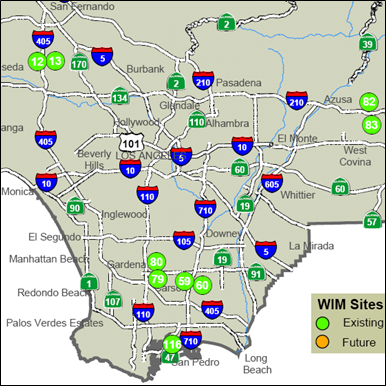
Figure 4-12. Coverage of (top) WIM stations and (bottom) vehicle detector stations in Los Angeles

4.4.1. Data Sources and Characteristics

Three traffic data sources in California were used. Each of them has different characteristics and provides a different type of data. They are described briefly below.

Freeway Performance Measurement System (PeMS)

PeMS is an interactive system that allows users to query various performance measures of the major freeways in California historically and in real-time [Choe et al., 2002]. The system consists of numerous embedded loop detectors, each reporting flow and lane occupancy and thus allowing average traffic speed to be estimated [Kwon, 2004]. These data are gathered through local Traffic Management Centers (TMCs), and then filtered, processed, and made accessible at 30-second intervals via the PeMS server, or at 5-minute intervals on the PeMS website (https://pems.eecs.berkeley.edu/).

The main advantage of PeMS is its large coverage, both spatially and temporally. The system covers more than 30,000 directional freeway miles throughout the state and the historical data for some freeways are available back to the late 90's. Although the data from PeMS includes a certain amount of uncertainty (e.g. when loop detectors are malfunctioning), it is still considered one of the most comprehensive and reliable data sources currently available in California.

In this study, PeMS is used to provide data of average traffic speed, total flow, and truck flow. The total flow reported by PeMS is from direct measurement, but the truck flow is based on estimation [Kwon et al., 2003]. It should be noted that the average traffic speed reported by PeMS is for overall traffic (i.e. all vehicles in the traffic stream). PeMS does not report separate speed values for different vehicle types.

Weigh-In-Motion (WIM) Stations

In California, WIM sensors consist of either bending plates on frames embedded in concrete or piezo sensors epoxied into the pavement. Inductive loops are placed before and after the WIM sensor array. These double-loops measure vehicle speed and overall length. Smooth pavement and proper calibration ensures quality and consistency in weight data. The calibration must be performed to +/- 5% accuracy with a test vehicle of known static weight driven at various highway speeds over the WIM instrumentation. For more information about WIM stations in California, see http://www.dot.ca.gov/hq/traffops/trucks/datawim/index.html.

WIM stations provide various data on vehicle and traffic characteristics, including vehicle class, gross vehicle weight, axle weight, axle spacing, vehicle speed, etc. It should be noted that the WIM stations in California use a similar vehicle classification system to the HPMS' classification system. However, they do not record data for passenger vehicles (classes 1-3) and have one additional HDT class (class 14) as depicted in Figure 4-13. In this research, raw data for individual vehicles were obtained. Classes 8-10 are considered single-unit trucks (source types 52 & 53 in MOVES) and classes 11-13 are considered combination trucks (source types 61 & 62 in MOVES).

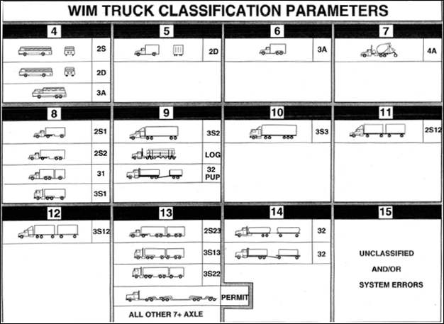
Figure 4-13. Vehicle classification system used by WIM stations in California

4.4.2. Data Fusion Method

Data fusion is the combining of data from multiple sources such that the resulting information is better than would be possible when these sources were used individually. The resulting information can be better in several ways such as being more accurate, less ambiguous, more complete, and more robust. Many data fusion techniques have been used in traffic engineering applications, for example, Kalman filter [Kim et al., 2007], Bayesian theory [Choi and Chung, 2002], neural network [Cheu et al., 2001], and fuzzy logic [Choi and Chung, 2002]. These techniques were reviewed but were considered to be unsuitable for the purpose of this subtask of the research, which is to combine data from WIM stations and VDS by making use of truck weight information from WIM stations in generating HDT activity data inputs for MOVES on the basis of vehicle OpMode distribution.

Therefore, a data fusion method based on data association concept, which correlates one set of observations with another set of observations, was developed. In this subsection, the developed data fusion method is presented using the freeway system in Los Angeles County, California, as an example. Figure 4-14 shows the flow chart of the developed data fusion method.

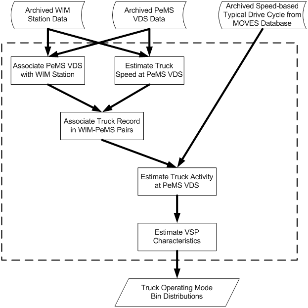
Figure 4-14. Flow chart of the proposed data fusion method

Data Screening

There are 20 WIM stations in both directions of the freeways in Los Angeles County. Based on the health report of these WIM stations, only 11 of them are functional. These stations include VAN NUYS (SB/NB) along I-405, CASTAIC (SB/NB) along I-5, LA 710 (SB/NB) along I-710, ARTESIA (EB/WB) along SR-91, GLENDORA (EB/WB) along I-210, and LONG BEACH PORT along SR-47. Figure 4-15 shows the locations of the PeMS VDS (mainline only) and the selected 11 WIM stations in the Los Angeles County. Note that there are five WIM stations that are located at the same location as another station, but in the opposite direction of the freeway, which may not be easily identified in Figure 4-15.

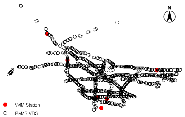
Figure 4-15. Locations of 1466 PeMS VDS and the selected 11 WIM stations in the Los Angeles County.

As to the one-year WIM data from July 2008 to June 2009, the following can be observed on the healthy condition:

• WIM data at CASTAIC (SB/NB) are not good for use across the year due to "restriped lanes";
• LA 710 NB always reports higher values in both class and weight than ground truth;
• Since November 2008, measurement with positive systematic bias has been reported at LA 710 SB;
• WIM data at ARTESIA (EB/WB) were not available until the completion of construction in March 2009;
• At some stations, classification data could be erroneous in a certain month while weight data may not be correct during another month;
• There is not any month with all 11 WIM stations being healthy for both classification and weight measurement. April 2009 or May 2009 has been considered the best candidate in terms of the number of healthy study sites (totally 6 sites), including VAN NUYS (SB) along I-405, ARTESIA (EB/WB) along SR-91, GLENDORA (EB/WB) along I-210, and LONG BEACH PORT along SR-47.

The examination of the PeMS VDS health condition reveals that good data accounts for a slightly higher percentage in April 2009 than in May 2009 (66.2% vs. 64.3%). Figure 4-16 shows a plot on the day-to-day health condition for all mainline VDS in District 7 (including the Los Angeles county and the Ventura county). Table 4-9 provides more detailed information on detector health for both April and May 2009. Therefore, WIM data and PeMS VDS data in April 2009 are used in the following analyses.

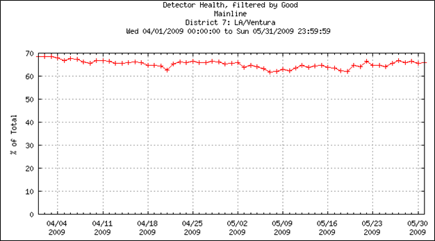
Figure 4-16. Day-to-day health condition for all mainline VDS in District 7 from April 1^st, 2009 to May 31^st, 2009.

Table 4-9. Summary of mainline VDS health in District 7 for April and May 2009

Month	Good	Line Down	Controller Down	No Data	Insufficient Data	Card Off	High Value	Intermittent	Constant	Feed Unstable
April	66.2	7.3	11.0	2.9	1.7	6.6	3.2	1.1	0.0	0.0
May	64.3	7.3	11.9	3.4	1.9	6.5	3.7	1.0	0.0	0.0

WIM Station and PeMS VDS Association

The next step is to determine the association between PeMS VDS with each candidate WIM station. Figure 4-17 illustrates a flow chart for a set of heuristic association rules. For each VDS, the closest WIM station (in terms of route distance) along the same freeway in the same direction is associated. If not available, then the closest WIM station (in terms of route distance) along the same freeway in the opposite direction is associated. If still not available, then the closest station (in terms of Euclidean distance) within the study region is associated.

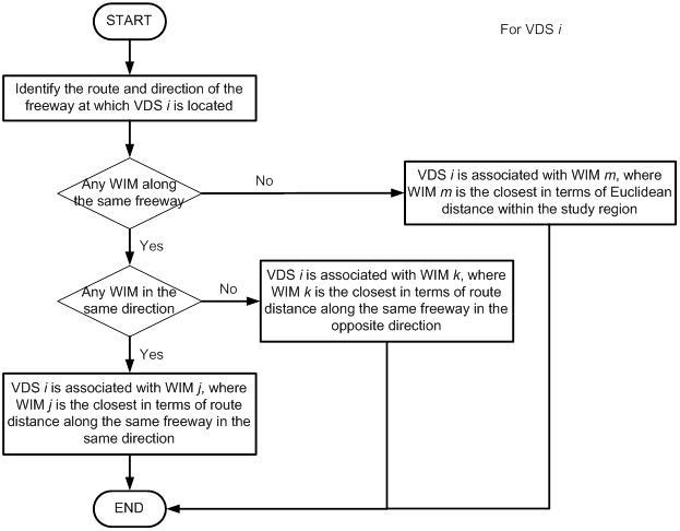
Figure 4-17. WIM station and PeMS VDS association rules.

Truck Record Association

At each WIM station, any truck passing by is logged with several information including time stamp, class, weight, speed, number of axles, etc. On the other hand, truck volume (without any detailed estimated arrival time) within a certain time interval (e.g. 5 minutes) at each VDS is estimated and archived in PeMS. However, it should be noted that even though each VDS can be associated with one WIM station using the set of rules above, it does not mean that every recorded truck in one WIM station will have a footprint on the associated VDS at some time point and vice versa. That is, not all truck passing by a VDS can be traced back to a specific record from the associated WIM station. This is because:

1. There are a very limited number of WIM stations within the study scope and some trucks may not be recorded by any WIM stations;
2. The truck volume recorded at each PeMS VDS is an estimated value instead of ground truth using the well-known g-factor method; and
3. There is no prior knowledge on the route of each truck or truck signature information among different WIM stations.

Due to the limitation mentioned above, a heuristic truck record association strategy is developed based on the following assumptions:

• There is no measurement error in the record from each WIM station;
• There is no estimation error in the record from each PeMS VDS;
• The "first-in-first-out (FIFO)" rule applies to the association strategy, i.e. no over-take is allowed;
• At each time interval, the truck weight and classification distribution at every PeMS VDS is the same as a certain consecutive set of truck record from the associated WIM station.

The basic idea of the proposed truck record association strategy is that based on the truck volume recorded at each PeMS VDS during each time interval and the estimated travel time distribution of each recorded truck from the associated WIM station under prevailing traffic condition, the same number of recorded trucks of the WIM station with the maximum likelihood are associated with the record at the PeMS VDS during the specified time interval. This is only to say the number of trucks matches with each other between a PeMS VDS and the associated WIM station, which can be called "weak" association. It is not meant to say each truck record matches with each other between a PeMS VDS and the associated WIM station, which is called &quot;strong&quot; association. According to the discussion above, it is self-evident that conducting &quot;strong&quot; association in this study is meaningless due to the lack of detailed information and too computationally demanding as well. So, &quot;weak&quot; association is conducted in the current study.

Numerous studies have focused on the estimation of travel time based on loop detector data [Chen et al., 2003; Coifman, 2002; Ni and Wang, 2008].Some of them use vehicle re-identification technique, while others recursively estimate vehicle trajectories given hypothetic trip starting time and then calculate the travel time. However, these strategies may not be applicable to this study due to the computational load. For simplicity, during time interval , the estimated (mode) travel time between the i-th PeMS VDS and its associated WIM station is calculated as

where represents the route distance between VDS i and its associated WIM station; and denotes the average truck speed between the i-th PeMS VDS and the VDS closest to the associated WIM station at time interval k. It needs to be pointed out that the calculation of route distance between a VDS and the associated WIM station is far from being trivial if the associated WIM station is not located at the same freeway as that VDS. A geographic information system (GIS) has to be used and a large database needs to be explored to determine . In addition, a PeMS VDS only provides speed estimate for overall traffic flow without differentiating the truck flow. [Boriboonsomsin et al., 2011] analyzed the truck data from 15 WIM stations and traffic data from the corresponding closest PeMS VDS in Southern California, and pointed out that there is a strong linear relationship between truck speed and overall traffic speed although the linear coefficient may vary from site to site. In this study, therefore, truck speed is estimated based on the results from [Boriboonsomsin et al., 2011].

Due to uncertainties, actual travel time should be a random variable. Generally speaking, estimation of travel time distribution is very challenging [Wan, 2011]. [Rakha et al., 2006] argued that although the travel time data collected from a section of I-35 South failed the goodness-of-fit tests for the Normal and lognormal distributions due to outlier observation at the tail, these distributions should be considered reasonable from a practical standpoint. In this study, a one-sided truncated symmetric distribution (say, Normal distribution) is used as the estimate of travel time distribution, where the truncated values are governed by the shortest possible truck travel time

where mph is set for all VDS as the maximum limit of truck speed.

Considering all ingredients discussed above, a heuristic truck record association method is proposed as follows. Without loss of generality, given the truck volume, n, at the i-th downstream PeMS VDS during the time interval k, n consecutive recorded trucks from the associated WIM station will be selected for association whose recorded arrival times are the closest (from both sides) to the time point, , by taking into account the truncation effect. And

where represents the mid-point of time interval k, e.g. is 08:02:30 for the time interval between 08:00:00 and 08:05:00. Figure 5 presents an example of truck record association for a case where the truck volume at the i-th downstream PeMS VDS. The "circles" depict the recorded arrival time of trucks at the WIM station and those "circles" in red denotes the associated recorded trucks. The curve f represents a hypothetical travel time distribution with one tail being truncated by .

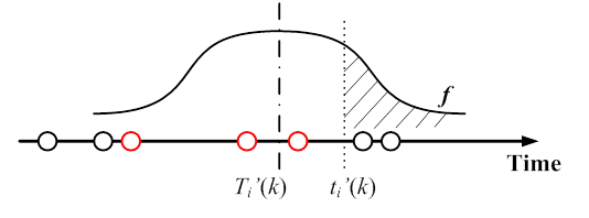
Figure 4-18. An illustrative example of truck record association method

Truck Activity Estimation

After the truck record has been associated for each PeMS VDS during every time interval, second-by-second truck activities can be estimated from the drive schedule defined in MOVES [U.S. Environmental Protection Agency, 2010] based on source type, roadway type and average speed. Table 4-10 and Table 4-11 list default driving cycles in MOVES for single-unit trucks and combination trucks, respectively [U.S. Environmental Protection Agency, 2010]. These driving cycles have approximate average speed from 5 mph to 70 mph. Note that driving cycle IDs 206 and 306 were not used in this study as driving cycle IDs 251 and 351 were already used to represent 30-mph freeway driving.

The speed profile and joint speed-acceleration frequency distribution of driving cycle ID 354 are illustrated in Figure 4-19. The speed profiles and joint speed-acceleration frequency distributions of other driving cycles are given in Appendix E.

Table 4-10. MOVES driving cycles for single-unit trucks

ID	Cycle Name	Average Speed (mph)	Non-Freeway		Freeway
			Rural	Urban	Rural	Urban
201	MD 5mph Non-Freeway	4.6	X	X	X	X
202	MD 10mph Non-Freeway	10.7	X	X	X	X
203	MD 15mph Non-Freeway	15.6	X	X	X	X
204	MD 20mph Non-Freeway	20.8	X	X	X	X
205	MD 25mph Non-Freeway	24.5	X	X	X	X
206	MD 30mph Non-Freeway	31.5	X	X	X	X
251	MD 30mph Freeway	34.4	X	X	X	X
252	MD 40mph Freeway	44.5	X	X	X	X
253	MD 50mph Freeway	55.4	X	X	X	X
254	MD 60mph Freeway	60.4	X	X	X	X
255	MD High Speed Freeway	72.8	X	X	X	X

Table 4-11. MOVES driving cycles for combination trucks

ID	Cycle Name	Average Speed (mph)	Non-Freeway		Freeway
			Rural	Urban	Rural	Urban
301	HD 5mph Non-Freeway	5.8	X	X	X	X
302	HD 10mph Non-Freeway	11.2	X	X	X	X
303	HD 15mph Non-Freeway	15.6	X	X	X	X
304	HD 20mph Non-Freeway	19.4	X	X	X	X
305	HD 25mph Non-Freeway	25.6	X	X	X	X
306	HD 30mph Non-Freeway	32.5	X	X	X	X
351	HD 30mph Freeway	34.4	X	X	X	X
352	HD 40mph Freeway	47.1	X	X	X	X
353	HD 50mph Freeway	54.2	X	X	X	X
354	HD 60mph Freeway	59.4	X	X	X	X
355	HD High Speed Freeway	71.7	X	X	X	X

 

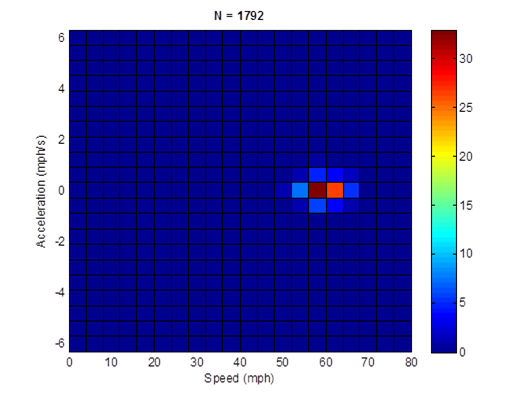
Figure 4-19. HD 60mph freeway cycle (length = 1,792 seconds; average speed = 59.4 mph)

The truck activity estimation method is described as follows:

1. Based on the estimated truck speed, two MOVES driving cycles whose average speeds are the closet to the estimated speed and bracket it will be selected for later acceleration generation. For example, if the estimated truck speed is 55 mph, then Driving Cycle #353 (average speed of 54.2 mph) and #354 (average speed of 59.4 mph) are selected.
2. Obtain the typical second-by-second acceleration distribution vs. different bin of speed for the selected driving cycles. This can be done by applying the Central Difference Method to those second-by-second speed data.
3. Determine the second-by-second acceleration by randomly picking a value from those two selected driving cycles. The probability for selecting whichever cycle is governed by the difference between the estimated speed and the average speed of each driving cycle. For the same example mentioned above, the probability of choosing an acceleration value from Driving Cycle #353 is 0.846 while 0.154 for the other. So Driving Cycle #353 is more likely to be selected as a target acceleration pool.
4. Uniformly randomly sample an acceleration value from the target sample pool to get the estimate of acceleration for each second and calculate the speed for the next second. Care needs to be taken to select the acceleration sample from the associated speed bin which is comparable to the speed estimation of the current step. Otherwise, the speed value could drift out of the range of those bracketed Driving Cycles. In this study, the size of speed bin is chosen as 2 mph.
5. Set the initial speed as the estimated truck speed from the PeMS VDS and keep looping on step 3) and 4) until the end of temporal span of the truck's foot-print at the VDS during the time interval. Such temporal span can be estimated by

where refers to the effective length of VDS i (see Figure 4-20); is the estimated truck speed at VDS i in the k-th time interval; anda is the length of each time interval (e.g. 5 minutes).

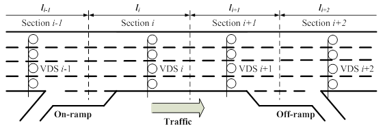
Figure 4-20. Layout of detectors and illustration of effective lengths along a freeway section.

VSP Calculation and Binning

With the estimate of second-by-second activity (including both speed and acceleration) for each truck as well as the information on vehicle class and weight, the vehicle specific power (VSP) or Scaled Tractive Power (STP) characteristics for trucks in kWatt/tonne can be calculated using the following formula [Gururaja, 2011].

where , and are the road-load related coefficients for rolling resistance (), rotating resistance () and aerodynamic drag (), respectively; is the vehicle speed (m/sec); is the mass of truck (metric ton); is the vehicle acceleration (meter/sec²); and is the fixed mass factor for the source type (kg); [U.S. Environmental Protection Agency, 2010] provides recommendation on the values of these parameters. In addition, the road grade is assumed to be zero in this study.

After the STP values were calculated, they were binned according to the U.S. EPA's vehicle operating model bin definition, shown in Figure 4-21.

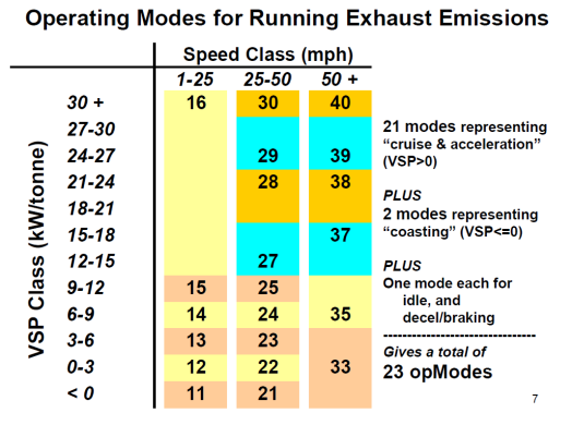
Figure 4-21. Vehicle operating mode bin definitions for heavy-duty trucks

4.4.3. Numerical Example

Truck Record Association

On Wednesday April 15^th, 2009, there were 12 trucks estimated to pass by VDS #718479 during the 5-minute period from 00:40:00 to 00:45:00. The estimated overall traffic speed at this VDS is 66.2 mph and the estimated truck speed is

66.2*0.863 = 57.1 mph.

where 0.863 is the coefficient for the linear relationship between the truck speed and overall traffic speed derived from a previous study [Boriboonsomsin et al., 2011]. Since the effective length of this VDS is 0.33 mile, the temporal foot-prints of these trucks at this VDS during this 5-minute period is

min(round(0.33/57.1*3,600), 300) = 21 seconds.

The VDS #718479 is associated with the Van Nuys WIM station on the same freeway (I-405) in the same direction (southbound). Figure 4-22 depicts the locations of the Van Nuys WIM station (Point A) and the VDS #718479 (Point B).

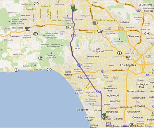
Figure 4-22. Locations of the WIM station (Point A) and the VDS (Point B)

The VDS is located 24.7 miles downstream of the WIM station. The closest VDS to the WIM station is VDS #767366. At this VDS, the recorded overall traffic speed from 00:40:00 to 00:45:00 is 71.7 mph and the estimated truck speed is

71.7*0.863 = 61.9 mph.

Therefore, the average speed used for the association is

(57.1+61.9)/2 = 59.5 mph.

And the estimated travel time is

24.7/59.5*3,600 = 1,495 seconds or 24 min 55 seconds.

Note that the maximum truck speed is set as 70 mph, so the minimum travel time is

24.7/70*3,600 = 1,270 seconds or 21 min 10 seconds

Therefore, starting from the mid-point (00:42:30) of the time period between 00:40:00 and 00:45:00, we checked the vehicle records from the WIM station before 00:21:20 and selected 12 vehicles whose arrival times are closest to 00:17:35. Table 4-12 shows the sample vehicle records from the Van Nuys WIM station on Wednesday April 15^th, 2009. The 12 vehicle records that were selected are in boldface:

Table 4-12. Sample truck records from the WIM station on Wednesday April 15th, 2009

Date	Time	Class	Weight (kg)
4/15/2009	00:11:07	9	2.99E+04
4/15/2009	00:11:37	5	3.76E+03
4/15/2009	00:12:08	14	9.71E+03
4/15/2009	00:12:53	9	1.57E+04
4/15/2009	0:13:25	9	2.37E+04
4/15/2009	0:14:07	11	2.35E+04
4/15/2009	00:15:02	3	2.90E+03
4/15/2009	00:15:37	9	1.32E+04
4/15/2009	00:16:01	9	1.28E+04
4/15/2009	00:17:35	Best Estimated Arrival Time at WIM
4/15/2009	00:18:45	9	1.29E+04
4/15/2009	00:18:48	9	1.26E+04
4/15/2009	00:19:33	9	1.36E+04
4/15/2009	00:19:46	9	9.71E+03
4/15/2009	00:19:47	9	1.13E+04
4/15/2009	00:20:23	9	1.06E+04
4/15/2009	00:20:29	5	5.67E+03
4/15/2009	00:22:20	6	1.18E+04
4/15/2009	00:23:32	9	1.43E+04
4/15/2009	00:25:59	9	2.26E+04
4/15/2009	00:26:28	9	1.04E+04

Effect of Truck Information on Operating Mode Estimation

Using the data described above, we investigated the effect of detailed truck information on the operating mode estimation. For those 12 recorded vehicles, there were two vehicles not belonging to the vehicle classes of interest (i.e., Classes 8 to 13). Of the remaining 10 vehicles (trucks), only 1 truck was a combination truck while the rest were single-unit trucks. Note that if detailed vehicle records such as shown above are not available, other data sources may be used or an assumption may be made regarding the fraction between single-unit and combination trucks. For example, based on the analysis of the WIM data from all WIM stations in the Los Angeles area in April 2009, it was found that among all the trucks belonging to Classes 8 through 13, single-unit trucks (Classes 8-10) accounted for 92% while combination trucks (Classes 11-13) accounted for 8%.

As stated earlier, the estimated average truck speed at VDS #718479 is 57.1 mph. In a procedure used by MOVES, this average truck speed information is first used to identify two default driving cycles whose average speeds bound the average truck speed. In this example, these are driving cycle IDs 253 (average speed of 55.4 mph) and 254 (average speed of 60.4 mph) for single-unit trucks, and driving cycle IDs 353 (average speed of 54.2 mph) and 354 (average speed of 59.4 mph) for combination trucks. Then, a vehicle OpMode distribution is determined by calculating a weighted average between the distributions of the two bracketing driving cycles. No truck weight information is used.

For instance, the vehicle OpMode distributions of driving cycle IDs 253 and 254for single-unit trucks are shown in Figure 4-23. Then, the top plot in Figure 4-24 shows the vehicle OpMode distribution of the single-unit trucks of interest that is calculated by the weighted average method. It is clearly shown that the pattern of the distribution assimilates that of the two distributions it is created from. On the other hand, the vehicle OpMode distribution created by the method proposed in this study (shown in the bottom plot of Figure 4-24) has a distinctively different pattern. Although the dominant bin is Bin 33 for both methods, the proposed method has a significantly higher fraction of truck activity in Bin 35 while there is no truck activity in Bins 11, 12, 21, 22, and 23 as in the weighted average method. The differences are contributed mainly by the use of actual truck weight information in the proposed method.

Similarly, the vehicle OpMode distributions of driving cycle IDs 353 and 354for combination trucks are shown in Figure 4-25. Then, the top plot in Figure 4-26 shows the vehicle OpMode distribution of the combination truck of interest that is calculated by the weighted average method, which assimilates the two distributions it is created from. Again, the vehicle OpMode distribution created by the method proposed in this study (shown in the bottom plot of Figure 4-26) has a distinctively different pattern where all the truck activity is in only three bins, which are Bins 33, 35, and 37.

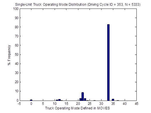
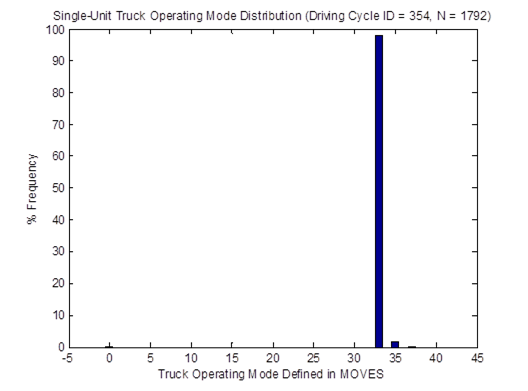
Figure 4-23. Vehicle OpMode distributions for single-unit trucks for driving cycle ID 253 (top) and driving cycle ID 254 (bottom)

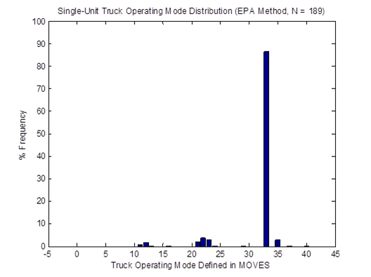
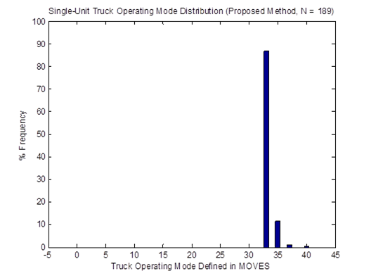
Figure 4-24. Vehicle OpMode distributions for single-unit trucks for the weighted average method (top) and the proposed method (bottom)

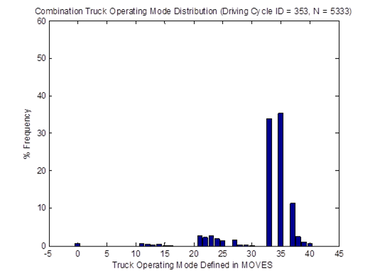
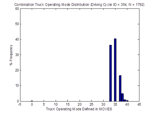
Figure 4-25. Vehicle OpMode distributions for combination trucks for driving cycle ID 353 (top) and driving cycle ID 354 (bottom)

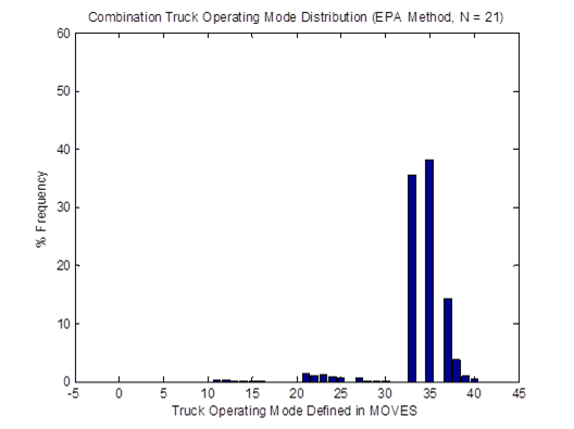
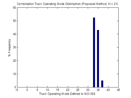
Figure 4-26. Vehicle OpMode distributions for combination trucks for the weighted average method (top) and the proposed method (bottom)

4.4.4. Results and Discussion

VSP distributions and vehicle OpMode distributions were created for single-unit trucks and combination trucks on freeways in the Los Angeles County using the entire month of data in April 2009. These distributions were created using both the proposed method and the weighted average method used by MOVES that were discussed in the numerical example. The distributions were also created separately for weekdays and weekends.

Figure 4-27 and Figure 4-28 show the VSP distributions for single-unit trucks for weekdays and weekends, respectively. Similarly, Figure 4-29 and Figure 4-30 show the VSP distributions for combination trucks for weekdays and weekends, respectively. In all the figures, the distributions created by both methods are shown. It is observed that in every case, the VSP distributions created by both methods follow the Gaussian distribution. However, the ones created by the proposed method have higher variation, which is due to the variation of truck weight used in the calculation of VSP.

Figure 4-31 and Figure 4-32 show the vehicle OpMode distributions for single-unit trucks for weekdays and weekends, respectively. Similarly, Figure 4-33 and Figure 4-34 show the vehicle OpMode distributions for combination trucks for weekdays and weekends, respectively. In all the figures, the distributions created by both methods are shown. It is observed that for single-unit trucks, the shape of the distributions created by both methods is similar to each other although the scale is different. This is true for both weekdays and weekends. However, for combination trucks, both the shape and the scale of the distributions created by the two methods are very different. The weighted average method has a single dominant bin, which is Bin 33. On the other hand, the proposed method has two dominant bins, which are Bins 33 and 35 where Bin 35 also accounts for a higher fraction.

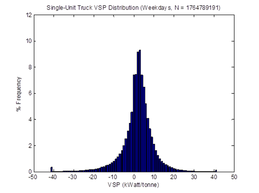
Figure 4-27. VSP distributions for single-unit trucks on weekdays in April 2009 (SHO = 29,413,153 hours) based on the proposed method (top) and the weighted average method (bottom).

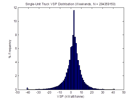
Figure 4-28. VSP distributions for single-unit trucks on weekends in April 2009 (SHO = 4,905,986 hours) based on the proposed method (top) and the weighted average method (bottom).

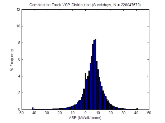
Figure 4-29. VSP distributions for combination trucks on weekdays in April 2009 (SHO = 3,800,795 hours) based on the proposed method (top) and the weighted average method (bottom).

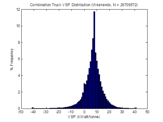
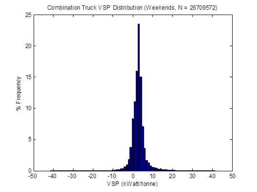
Figure 4-30. VSP distributions for combination trucks on weekends in April 2009 (SHO = 445,160 hours) based on the proposed method (top) and the weighted average method (bottom).

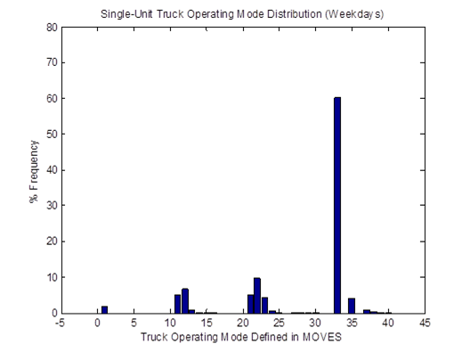
Figure 4-31. Vehicle OpMode distributions for single-unit trucks on weekdays in April 2009 (SHO = 29,413,153 hours) based on the proposed method (top) and the weighted average method (bottom).

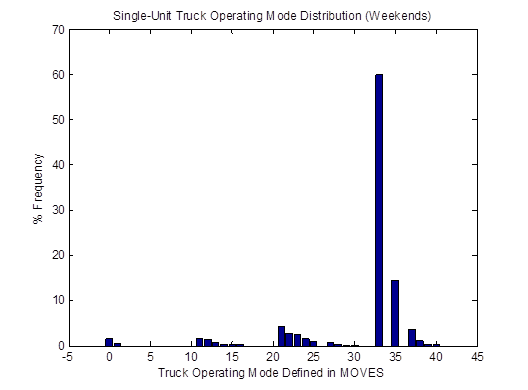
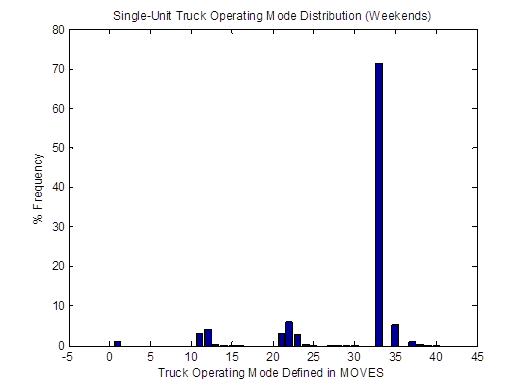
Figure 4-32. Vehicle OpMode distributions for single-unit trucks on weekends in April 2009 (SHO = 4,905,986 hours) based on the proposed method (top) and the weighted average method (bottom).

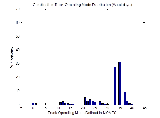
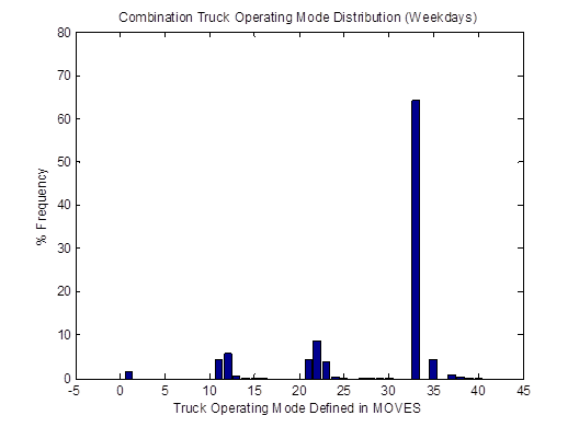
Figure 4-33. Vehicle OpMode distributions for combination trucks on weekdays in April 2009 (SHO = 3,800,795 hours) based on the proposed method (top) and the weighted average method (bottom).

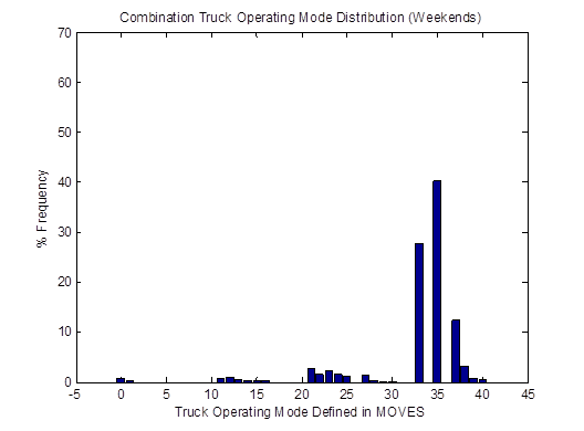
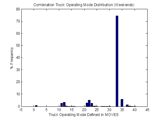
Figure 4-34. Vehicle OpMode distributions for combination trucks on weekends in April 2009 (SHO = 445,160 hours) based on the proposed method (top) and the weighted average method (bottom).

4.5. Concluding remarks

An accurate characterization of vehicle activity is crucial to the construction of regional emissions inventory of on-road mobile sources for use in SIPs and transportation conformity analyses. However, it is a challenging task given the limited availability of vehicle activity data at a large, regional scale. Compared to light-duty vehicles, the availability of vehicle activity data of HDTs are even more limited. This research examines the use of alternative sources of HDT activity data including truck's ECU and telematics-based vehicle tracking and monitoring system to generate HDT activity data inputs for MOVES.

4.5.1. Truck ECU Data

The advantages of truck's ECU data are that they can be acquired in a large amount with relatively low costs, and that they contain a number of vehicle and engine parameters that may also be useful for other purposes. However, their limitations include the fact that the data are aggregated over the lifetime of the truck or from the last time its ECU was reset, and have no detailed spatial or temporal information associated with them. For instance, ECU downloads can provide data regarding VMT, vehicle hours traveled (VHT), number of idling hours, and number of trips starts for an aggregate time period. However, these data cannot be differentiated by road type or area. Nevertheless, ECU downloads can be used to develop base data (e.g., total idling hours) from a large number of HDTs. Then, these base data can be disaggregated using spatial or temporal distribution factors derived from other small-scaled studies (e.g., GPS-based instrumented vehicle studies).

4.5.2. Truck Telematics Data

For the truck telematics data, they have several advantages. First, they include GPS information of the HDTs, which can be used to derive various forms of HDT activity data such as miles traveled, speed, trip starts, and idle time in detail. The use of GPS information also allows detailed activity data on unrestricted access roads, where the availability of traditional traffic sensors is limited, to be collected. Second, they are continuously collected, thus allowing temporal distributions of HDT activity to be developed by hour, day, and even month. Third, they can be obtained from a sizable number of HDT samples at a time, improving the confidence in the derived HDT activity data. As an example, the dataset used in this study includes data from more than 2,000 HDTs while the largest instrumented vehicle study of HDTs ever conducted in the U.S. has only 120 HDTs [Battelle, 1999]. Lastly, by coupling them with proper vehicle and fleet characterization, the truck telematics data can be used to develop vehicle activity data for specific truck groups (e.g., combination long-haul trucks of engine model year 2007 or later) based on their emission characteristics.

On the other hand, it is important to understand the limitations of the truck telematics data used in this study as well. First, they are collected at a much coarser interval (e.g., 30-second or 5-minute depending on the fleet) as compared to the data from instrumented vehicle studies, which are usually collected at a one-second interval. This may slightly affect the accuracy of the derived HDT activity data. Second, they are collected from a subset of HDTs in the total population. Thus, they cannot be used to derive the absolute statistics of the HDT population such as total VMT.

As shown in this report, the truck telematics data can be used to develop several of the HDT activity data inputs required by the EPA's MOVES model. Depending on the availability and quality of the existing data sources, the truck telematics data can be used to provide, supplement, or replace some of the required HDT activity data inputs developed from those existing data sources. For instance, if an area already has continuous traffic counters that differentiate traffic counts by vehicle type, then they can be used to develop VMT fraction by road type as well as by weekday/weekend and by hour, and the truck telematics data can be used to provide average speed distribution as well as trip starts location and distribution.

In addition to the several HDT activity data inputs required by the EPA's MOVES model, the truck telematics data can also be used generate other information for energy and emission analysis of HDTs. For example, link-based and area-based historical maps of truck fuel economy for a region can be generated based on this data set, which can be used to identify links or areas for capital improvement or traffic flow improvement projects.

4.5.3. Truck Data Fusion

This chapter also presents a method to fuse HDT datasets from WIM stations and vehicle detector stations (VDS) to result in more refined and accurate HDT activity data. The main idea is to identify trucks recorded by a WIM station that are likely to travel over a VDS during a time period. Then, the actual weight information of these trucks can be combined with the second-by-second speed and acceleration values from synthetic trajectories created from strategically selected MOVES default driving cycles to calculate the associated truck scale tractive power (STP) values. The STP values can then be binned by operating mode according to the U.S. EPA's definition.

This method should be more accurate than the current default method that assumes an average weight value for all the HDTs in the same class. This would result in more accurate emission inventories of HDTs, especially in areas that have freight terminals or freight corridors. The method relies on HDT weight information from WIM stations, which are available across the nation as depicted in Figure 4-35. Table 4-13 lists the top 20 MPOs that have the most number of WIM stations in their respective jurisdiction.

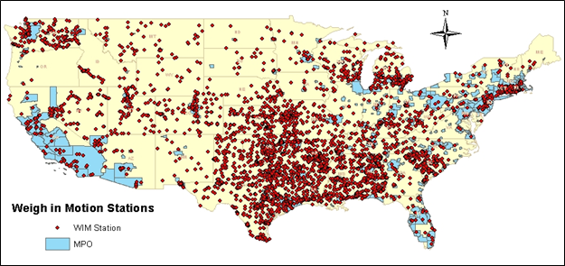
Figure4-35. WIM stations across the U.S.

Table 4-13. Top 20 MPOs with the most number of WIM stations

No.	Metropolitan Planning Organization	State	Population in Year 2000	No. of WIM Stations*
1	State Planning Council	RI	1,048,319	107
2	North Central Texas COG	TX	4,879,535	104
3	Mid-America Regional Council	MO	1,582,372	84
4	Houston-Galveston Area Council	TX	4,669,571	82
5	Regional Transportation Commission of Southern Nevada	NV	1,375,765	73
6	Southeast Michigan COG	MI	4,833,493	56
7	Denver Regional COG	CO	2,394,504	40
8	Association of Central Oklahoma Governments	OK	990,564	40
9	Puget Sound Regional Council	WA	3,275,847	37
10	Southern California Association of Governments	CA	16,516,006	36
11	Louisville Area MPO	KY	968,313	31
12	Capital Area MPO	TX	1,159,836	30
13	San Antonio-Bexar County MPO	TX	1,415,906	26
14	Metropolitan Transportation Commission	CA	6,783,760	24
15	North Jersey Transportation Planning Authority	NJ	6,310,989	24
16	Cincinnati-Northern Kentucky MPO	OH	1,868,835	20
17	Southeastern Wisconsin Regional Planning Commission	WI	1,932,908	19
18	Birmingham MPO	AL	805,340	18
19	Delaware Valley Regional Planning Commission	PA	5,387,407	16
20	Wasatch Front Regional Council	UT	1,328,198	13

*Source: http://www.bts.gov/publications/national_transportation_atlas_database/2011/

Updated: 6/28/2017