

- Highway Scenario Implications
- Linkage Between Recent Conditions and Performance and Spending Trends and Selected Capital Investment Scenarios
- Operational Performance
- Physical Conditions
- Historic and Projected Travel Growth
- Historic Travel Growth
- Travel Growth Forecasts
- Accounting for Inflation
- Timing of Investment
- Highway and Bridge Investment Backlog
- Alternative Timing of Investment in HERS
- Alternative Timing of Investment in NBIAS
- Timing of Congestion Pricing
- Linkage Between Recent Conditions and Performance and Spending Trends and Selected Capital Investment Scenarios
- Transit Scenario Implications
- Ridership Response to Investment
- Impact of Congestion Pricing on CO2 Emissions
- Transit Travel Growth
- Historic Transit Travel Growth
- Transit Travel Growth Forecasts
- Projected and Historical Transit Travel Growth
- Commodity Inflation
- Comparison
- Highways and Bridges
- Transit
Highway Scenario Implications
This section provides additional discussion on key issues relating to the relationship between highway capital investment and the conditions and performance of the system to assist in the interpretation of the future capital investment scenarios for highways and bridges presented in Chapter 8. This includes an analysis of the impacts that recent and historic funding patterns identified in Chapter 6 have had on the highway conditions and performance trends reported in Chapters 3 and 4, particularly in light of the levels and composition of capital investment associated with the future capital investment scenarios presented in Chapter 8. This section also compares historic growth in vehicle miles traveled (VMT) with the State-generated travel forecasts that underlie the investment/performance analyses presented in this report and illustrates the potential impacts of alternative rates of future construction cost inflation. This section also analyzes the potential impacts of alternative assumptions regarding the timing of investments and the implementation of congestion pricing.
Linkage Between Recent Conditions and Performance and Spending Trends
and Selected Capital Investment Scenarios
As discussed in Chapter 6, capital spending by all levels of government increased by 62.7 percent between 1997 and 2006, from $48.4 billion to $78.7 billion, but did not keep pace with the 69.4 percent increase in the Federal Highway Administration Composite Bid Price Index (BPI) over this period. This was primarily due to a sharp increase in the cost of construction materials between 2004 and 2006. In constant dollar terms, combined public and private highway capital spending fell by 4.0 percent between 1997 and 2006. Investment in system expansion (such as the widening of roads and the construction of new facilities) decreased by 14.2 percent in constant dollar terms over this period, while funding for system rehabilitation and system enhancement grew in constant dollar terms by 0.4 percent and 22.7 percent, respectively.
It is important to note that the overall decline in constant dollar capital spending for the period identified above is largely the result of the 40.3 percent increase in the BPI between 2004 and 2006. As indicated in the 2004 C&P Report, capital spending grew 22.9 percent in constant dollar terms between 1997 and 2004. There is a sometimes a delay between the point at which outlays are made and the point at which their impacts are quantifiable (i.e., partial payments on a complex project may have no impact until the project is completed and the road or bridge lane is opened or reopened to traffic). For this reason, the effect of these recent price increases on system conditions and performance may not yet be fully discernable.
Operational Performance
The analyses presented in Chapter 8 suggest that current highway investment levels would not be sufficient to sustain the operational performance of the highway system unless congestion pricing were broadly adopted. The $30.0 billion identified in Chapter 6 as capital spending by all levels of government for system expansion in 2006 is well below the $40.0 billion system expansion component of the fixed rate user financing version of the Sustain Conditions and Performance scenario, having fallen significantly in constant dollar terms as noted above. This finding is consistent with the recent declines in operational performance noted in Chapter 4 based on statistics computed using the methodology from the Texas Transportation Institute's 2005 Urban Mobility Study. The Average Daily Percentage of VMT Under Congested Conditions in urbanized areas increased from 27.4 percent in 1997 to 31.6 percent in 2006. For the period from 1997 to 2005, the Average Length of Congested Conditions in urbanized areas increased from 6.2 hours to 6.6 hours, while the estimated Annual Person-Hours of Delay in those areas rose from 3.3 billion hours in 1997 to 5.1 billion hours in 2005.
| Why do the comparisons of recent conditions and performance trends and recent spending trends focus on the fixed rate user financing versions of the Chapter 8 scenarios? | |
|
Congestion pricing has not been adopted on the widespread basis assumed for the variable rate user financing versions of the Chapter 8 scenarios. The fixed rate user financing versions are more consistent with how highway spending is currently financed, and should provide better benchmarks for examining the impacts of recent spending on recent system performance.
|
|
Physical Conditions
Although investment in system rehabilitation has increased slightly in constant dollar terms since 1997 despite recent sharp increases in construction costs, the analyses presented in Chapter 8 suggest that current highway investment levels are not sufficient to sustain the physical conditions of all parts of the highway system. The $40.4 billion identified in Chapter 6 as capital spending by all levels of government for system rehabilitation in 2006 is below the $43.5 billion system rehabilitation component of the fixed rate user financing version of the Sustain Conditions and Performance scenario, and the $47.0 billion system rehabilitation component of the fixed rate user financing version of the Sustain Conditions and Performance of System Components scenario. The funding gaps are most dramatic for lower-ordered urban functional systems, which is consistent with the findings reported in Chapter 3.
The share of urbanized collector VMT on pavements classified as having good ride quality decreased from 39.8 percent in 1997 to 35.6 percent in 2006. The comparable values for urbanized minor arterials fell from 40.8 percent to 33.7 percent over this same period; declines were also observed for rural major collectors, small urban collectors, and small urban minor arterials. The share of urbanized collector VMT on pavements classified as having acceptable ride quality decreased from 84.4 percent in 1997 to 72.9 percent in 2006; the comparable values for urbanized minor arterials fell from 83.3 percent to 74.9 percent over this same period. Declines were also observed for urbanized other principal arterials, small urban collectors, and small urban minor arterials. The overall share of VMT on pavements with acceptable ride quality for all systems for which data were available fell from 86.4 percent in 1997 to 86.0 percent in 2006 because the decreases noted above for lower-ordered systems were largely offset by increases for higher-ordered systems including the Interstate System.
The 2004 C&P Report indicated that spending in 2004 exceeded the estimated investment level for the bridge component of the "Cost to Maintain" scenario, which was consistent with the report's findings regarding reductions over time in the percent of deficient bridges. However, the $11.1 billion bridge component of the system rehabilitation investment levels identified as part of the Sustain Conditions and Performance scenario in Chapter 8 is higher than the $10.1 billion of combined public and private capital investment for bridge rehabilitation and replacement in 2006 cited in Chapter 6. Although Chapter 3 showed continued progress over time in the reduction of the percentage of bridges classified as deficient, from 34.2 percent in 1996 to 27.6 percent in 2006, these gains have not been as large in recent years and have not been consistent across all bridge performance measures. Between 2004 and 2006, the percent of deficient bridges on urban collectors rose slightly, as did the percent of travel on deficient National Highway System (NHS) bridges.
Historic and Projected Travel Growth
The Highway Performance Monitoring System (HPMS) data supplied by States is the source of the annual VMT statistics presented in this report, as well as the forecasts of future VMT used as input to the Highway Economic Requirements System (HERS) analysis. Separate 20-year forecasts are provided for each of the more than 119,000 HPMS sample sections, based on information that each State has available concerning the particular section and the corridor of which it is a part.
Historic Travel Growth
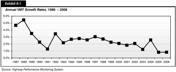
From 1986 to 2006, annual highway VMT increased from 1.85 trillion to 3.03 trillion, growing at an average annual growth rate of 2.52 percent. As shown in Exhibit 9-1, travel growth has varied somewhat from year to year, ranging from a high of 5.45 percent in 1988 to a low of 0.82 percent in 2005, and has generally been trending downward. For 10 out of these 20 years, annual VMT grew at a rate between 2 percent and 3 percent annually. Annual VMT growth exceeded 3 percent in 5 of these 20 years, and slowed to below 2 percent in another 5 of these years. As noted in Chapter 2, preliminary information for 2007 and early 2008 indicate that VMT growth may be negative in one or both of those years. Highway travel growth has typically been lower during periods of slow economic growth and/or higher fuel prices, and higher during periods of economic expansion.
Travel Growth Forecasts
The composite weighted average annual VMT growth rate based on the 20-year travel forecasts supplied by States with their 2006 HPMS sample section data is 1.84 percent. This is significantly below the average growth rate over the prior 20 years, although it is larger than the growth rates observed since 2004. Projected growth in rural areas (2.07 percent average annual) is somewhat higher than in urban areas (1.72 percent).
Exhibit 9-2 shows projected year-by-year VMT for the period 2006 to 2026 derived from these forecasts under two different assumptions about future growth patterns: geometric growth (growing at a constant annual rate) and linear growth (growing by a constant amount annually, implying that rates would gradually decline over the forecast period). The HERS analyses presented in this report used the linear growth assumption.
| Do the travel demand elasticity features in HERS differentiate between the components of user costs based on how accurately highway users perceive them? | |
|
No. The model assumes that comparable reductions or increases in travel time costs, vehicle operating costs, or crash costs would have the same effect on future VMT. The elasticity values in HERS were developed from studies relating actual costs to observed behavior; these studies did not explicitly consider perceived costs of individual user cost components.
Highway users can directly observe some types of user costs such as travel time and fuel costs. Other types of user costs, such as crash costs, can be measured only indirectly. In the short run, directly observed costs may have a greater effect on travel choice than costs that are harder to perceive. However, while highway users may not be able to accurately assess the crash risk for a given facility, they can incorporate their general perceptions of the relative safety of a facility into their decision-making process. The model assumes that the highway users' perceptions of costs are accurate, in the absence of strong empirical evidence that they are biased.
|
|
| Growth Pattern | Linear Growth (Constant Annual Amount) | Geometric Growth (Constant Annual Rate) |
|---|---|---|
| 2006 (actual) | 3,014 | 3,014 |
| 2007 | 3,080 | 3,069 |
| 2008 | 3,146 | 3,126 |
| 2009 | 3,213 | 3,183 |
| 2010 | 3,279 | 3,242 |
| 2011 | 3,345 | 3,301 |
| 2012 | 3,411 | 3,362 |
| 2013 | 3,477 | 3,423 |
| 2014 | 3,543 | 3,486 |
| 2015 | 3,609 | 3,550 |
| 2016 | 3,676 | 3,616 |
| 2017 | 3,742 | 3,682 |
| 2018 | 3,808 | 3,750 |
| 2019 | 3,874 | 3,818 |
| 2020 | 3,940 | 3,888 |
| 2021 | 4,006 | 3,960 |
| 2022 | 4,072 | 4,033 |
| 2023 | 4,139 | 4,107 |
| 2024 | 4,205 | 4,182 |
| 2025 | 4,271 | 4,259 |
| 2026 | 4,337 | 4,337 |
The HERS assumes that the HPMS forecasts represent the level of travel that would occur if a constant level of service were maintained and the cost of using the facility remain unchanged. As indicated in Chapter 7, this implies that travel will occur at this level only if pavement and capacity improvements made on the segment during the next 20 years are sufficient to maintain highway user costs at current levels throughout the 20 year period. The travel demand elasticity features in HERS assume that highway users will respond to increases in the cost of traveling a highway facility by shifting to other routes, switching to other modes of transportation, or forgoing some trips entirely. The model also assumes that reducing user costs on a facility will induce additional traffic on that route that would not otherwise have occurred. Future pavement and widening improvements would tend to reduce highway user costs and induce additional travel on the improved sections. If a highway section is not improved, highway user costs on that section would tend to rise over time because of pavement deterioration and/or increased congestion, thereby suppressing some travel on that section. Increases in fuel prices or other costs experienced by drivers would also tend to suppress travel below the HPMS baseline forecast.
One implication of travel demand elasticity is that each different scenario and benchmark developed using HERS results in a different projection of future VMT. Since higher investment levels generally result in reduced highway user costs, they also tend to result in higher levels of VMT growth. Another implication is that any external projection of future VMT growth will be valid only for a single level of investment in HERS. Thus, the baseline HPMS forecasts would be valid only under a specific set of conditions. Exhibit 7-6 in Chapter 7 identifies a range of projected 2026 VMT for different possible funding levels and financing mechanisms ranging from 4.187 trillion to 4.456 trillion; this would equate to average annual VMT growth rates of 1.62 percent to 1.94 percent.
Chapter 10 includes sensitivity analyses identifying the potential impacts of selected alternative travel demand forecasts on future system conditions and performance. The potential impacts of higher fuel prices are also explored.
Accounting for Inflation
The analyses of potential future investment/performance relationships reflected in the C&P report have traditionally been stated in constant dollars, with the base year set according to the year of the conditions and performance data supporting the analysis. As noted frequently in Chapters 7 and 8, all of the analyses in this edition are presented in constant 2006 dollars.
When applying these analytical findings in other contexts, such as comparing a particular scenario with nominal dollar revenue projections, it is sometimes necessary to adjust for inflation to ensure an accurate comparison. Such adjustments could be made by applying an assumption about future inflation to either convert the C&P report's constant dollar numbers to nominal dollars, or to convert the nominal projected revenues to constant 2006 dollars. Exhibit 9-3 illustrates how the constant dollar figures associated with the Interstate Sustain Conditions and Performance scenario presented in Chapter 8 could be converted to nominal dollars, based on three alternative inflation rates selected for their historical significance. The largest 20-year increase in the FHWA Composite BPI since 1956 occurred from 1960 to 1980, while the smallest 20-year increase occurred from 1980 to 2000; the average annual BPI increase for the former period was 7.4 percent, while the comparable annual rate for the latter period was 2.0 percent. From 1986 to 2006, the BPI grew at an average annual rate of 4.0 percent.
| Year | Interstate Sustain Conditions and Performance Scenario * Highway Capital Investment (Billions of Dollars) |
|||||||
|---|---|---|---|---|---|---|---|---|
| Assuming Fixed Rate User Financing (3.71 Percent Annual Constant Dollar Growth) |
Assuming Variable Rate User Financing (3.49 Percent Annual Constant Dollar Decline) |
|||||||
| Constant 2006 Dollars | Nominal Dollars Assuming 2.0 Percent Inflation |
Nominal Dollars Assuming 4.0 Percent Inflation |
Nominal Dollars Assuming 7.4 Percent Inflation |
Constant Dollar | Nominal Dollars Assuming 2.0 Percent Inflation |
Nominal Dollars Assuming 4.0 Percent Inflation |
Nominal Dollars Assuming 7.4 Percent Inflation |
|
| 2006 | $16.5 | $16.5 | $16.5 | $16.5 | $16.5 | $16.5 | $16.5 | $16.5 |
| 2007 | $17.2 | $17.5 | $17.8 | $18.4 | $16.0 | $16.3 | $16.6 | $17.1 |
| 2008 | $17.8 | $18.5 | $19.2 | $20.5 | $15.4 | $16.0 | $16.7 | $17.8 |
| 2009 | $18.5 | $19.6 | $20.8 | $22.9 | $14.9 | $15.8 | $16.7 | $18.4 |
| 2010 | $19.1 | $20.7 | $22.4 | $25.5 | $14.4 | $15.5 | $16.8 | $19.1 |
| 2011 | $19.8 | $21.9 | $24.1 | $28.4 | $13.8 | $15.3 | $16.9 | $19.8 |
| 2012 | $20.6 | $23.2 | $26.0 | $31.6 | $13.4 | $15.1 | $16.9 | $20.5 |
| 2013 | $21.3 | $24.5 | $28.1 | $35.2 | $12.9 | $14.8 | $17.0 | $21.3 |
| 2014 | $22.1 | $25.9 | $30.3 | $39.2 | $12.4 | $14.6 | $17.0 | $22.0 |
| 2015 | $23.0 | $27.4 | $32.7 | $43.6 | $12.0 | $14.4 | $17.1 | $22.8 |
| 2016 | $23.8 | $29.0 | $35.2 | $48.6 | $11.6 | $14.1 | $17.2 | $23.7 |
| 2017 | $24.7 | $30.7 | $38.0 | $54.1 | $11.2 | $13.9 | $17.2 | $24.5 |
| 2018 | $25.6 | $32.5 | $41.0 | $60.3 | $10.8 | $13.7 | $17.3 | $25.4 |
| 2019 | $26.6 | $34.4 | $44.2 | $67.2 | $10.4 | $13.5 | $17.4 | $26.4 |
| 2020 | $27.5 | $36.3 | $47.7 | $74.8 | $10.1 | $13.3 | $17.4 | $27.3 |
| 2021 | $28.6 | $38.4 | $51.4 | $83.3 | $9.7 | $13.1 | $17.5 | $28.3 |
| 2022 | $29.6 | $40.7 | $55.5 | $92.8 | $9.4 | $12.9 | $17.5 | $29.4 |
| 2023 | $30.7 | $43.0 | $59.8 | $103.4 | $9.0 | $12.7 | $17.6 | $30.4 |
| 2024 | $31.9 | $45.5 | $64.5 | $115.1 | $8.7 | $12.5 | $17.7 | $31.5 |
| 2025 | $33.0 | $48.1 | $69.6 | $128.2 | $8.4 | $12.3 | $17.7 | $32.7 |
| 2026 | $34.3 | $50.9 | $75.1 | $142.8 | $8.1 | $12.1 | $17.8 | $33.9 |
| Total | $495.6 | $628.8 | $803.6 | $1,236.1 | $232.6 | $281.6 | $344.0 | $492.4 |
| Average | ||||||||
| Annual | $24.8 | $11.6 | ||||||
The constant dollar figures for the Interstate Sustain Conditions and Performance scenario reflect the gradual ramping up of investment levels described in Chapter 7, and illustrated in Exhibit 7-2. As described in Exhibit 8-5, combined public and private highway capital investment would rise by 3.71 percent annually in constant dollar terms under the version of this scenario assuming fixed rate user financing, and would decrease by 3.49 percent annually in the variable rate user financing version of the scenario.
| Why are the investment analyses presented in this report expressed in constant base year dollars? | |
|
The investment/performance models discussed in this report estimate the future benefits and costs of transportation investments in constant dollar terms. This is standard practice for this type of economic analysis. To convert the model outputs from constant dollars to nominal dollars, it would be necessary to externally adjust them to account for projected future inflation.
Traditionally, this type of adjustment has not been made in the C&P report. As inflation prediction is an inexact science, adjusting the constant dollar figures to nominal dollars would tend to add to the uncertainty of the overall results, and make the report more difficult to use if the inflation assumptions were later proved to be incorrect. Allowing readers to make their own inflation adjustments based on actual trends observed subsequent to the publication of the C&P report and/or their the most recent projections from other sources is expected to yield a better overall result, particularly in light of recent sharp increases in highway construction materials costs that were not fully anticipated.
The use of constant dollar figures is also intended to provide readers with a reasonable frame of reference in terms of an overall cost level that they have recently experienced. When inflation rates are compounded for 20 years, even relatively small growth rates can produce nominal dollar values that appear very large when viewed from the perspective of today's typical costs.
The primary drawback to using constant base year dollar figures in the C&P report is that they are sometimes misapplied by readers, and treated as if they were expressed in current year dollars. However, as the C&P report is produced every two years, the base year costs reflected in the most recent edition are generally close enough to current costs to provide a useful perspective.
Inflation is but one of two separate and distinct factors that account for why the value of a dollar, as seen from the present, diminishes over time. The second factor is the time value of resources, which reflects that there is a cost associated with diverting the resources needed for an investment from other productive uses. The investment/performance models described in this report take the time value of resources into account via a separate mechanism called the discount rate, which is discussed in Chapter 10.
|
|
Assuming fixed rate user financing, the average annual capital spending level under this scenario of $24.8 billion in constant 2006 dollars corresponds to a 20-year total of $495.6 billion. Assuming a 2.0 percent annual increase in highway construction costs, this would translate into a nominal dollar figure of $628.8 billion; annual inflation of 7.4 percent would yield a nominal dollar figure of over $1.2 trillion.
Assuming variable rate user financing, the average annual capital spending level under this scenario of $11.6 billion in constant 2006 dollars corresponds to a 20-year total of $232.6 billion. Assuming a 2.0 percent annual increase in highway construction costs, this would translate into a nominal dollar figure of $281.6 billion; annual inflation of 7.4 percent would yield a nominal dollar figure of $492.4 billion.
While each project is different, States generally have faced increased prices for roadway construction and maintenance. As noted in Chapter 6, the BPI increased by 43.3 percent between 2004 and 2006, driven by large increases in the prices of steel, asphalt, and concrete. Worldwide demand from China, Europe, India, and the United States has put pressure on the refining and producing capacities for these construction materials. While anecdotal evidence suggests that some of these trends may be abating, it would not be surprising if highway construction costs continue to rise more quickly than consumer prices in the short term. Such increases can have significant impact on the ability of the public and private owners of the various components of the highway system to effectively manage the conditions and performance of these assets.
Timing of Investment
While the investment/performance analyses presented in this report focus mainly on how alternative average annual investment levels over 20 years might impact system performance at the end of that period, it is important to recognize that the timing of investment can have significant performance implications within this time period. As discussed in Chapter 7, the analyses for this report assumed that any increase or decrease in combined public and private investment would occur gradually, at a constant rate relative to 2006.
Although some previous editions of the C&P report included exhibits illustrating a gradual ramping up of spending levels, this was not consistent with the actual modeling assumptions in HERS and the National Bridge Investment Analysis System (NBIAS). The HERS analyses presented in the 2004 C&P Report were tied directly to alternative benefit-cost ratio cutoffs rather than to particular levels of investment in any given year. At higher spending levels, this approach resulted in a significant front-loading of capital investment in the early years of the analysis as the existing backlog of potential cost-beneficial investments was addressed, followed by a sharp decline in later years. The 2006 C&P Report assumed that combined public and private capital investment would immediately jump to the average annual level being analyzed, then remain fixed at that level for 20 years. In contrast, the baseline analyses presented in this report were constructed from HERS and NBIAS analyses that directly assumed a gradually ramping up or down in spending, depending on the investment level being analyzed.
Highway and Bridge Investment Backlog
The highway investment backlog represents all highway improvements that could be economically justified for immediate implementation, based on the current conditions and operational performance of the highway system. The HERS model estimates that a total of $523.5 billion of investment could be justified nationwide based solely on the current conditions and operational performance of the highway system. Approximately 86.1 percent of the backlog is in urban areas, with the remainder in rural areas. Capacity deficiencies on existing highways account for 46.2 percent of the backlog; the remainder results from pavement deficiencies. Approximately 57.6 percent of the backlog is on the NHS, while 34.5 percent of the backlog is on the Interstate highway system (a subset of the NHS).
The $523.5 billion dollar backlog figure noted above does not include the $98.9 billion economic bridge investment backlog figure computed by NBIAS and identified in Chapter 7. Combining these two figures yields a total highway and bridge investment backlog of $622.4 billion.
Note that the HERS-derived figure does not reflect rural minor collectors or rural and urban local roads and streets because HPMS does not contain sample section data for these functional systems; these systems are reflected in the NBIAS estimates. The combined backlog figure does not contain any estimate for system enhancements, which are not currently modeled. The HERS-derived figure assumes funding from non-user sources; the model is not currently equipped to compute a backlog assuming other financing mechanisms.
Alternative Timing of Investment in HERS
Exhibit 9-4 indicates how alternative assumptions regarding the timing of investment would impact the distribution of spending among the four 5-year funding periods considered in HERS. For the baseline analyses, the distribution of spending among funding periods is driven by the annual constant dollar spending growth rate assumed; for higher growth rates, a smaller percentage of total 20-year investment would occur in the first 5 years. When a 0-percent growth rate is assumed, one-quarter of total spending would occur in each of the 5-year funding periods.
| Baseline Annual Percent Change Relative to 2006 | Average Annual Spending Modeled in HERS (Billions of 2006 Dollars) 1 | Percentage of HERS-Modeled Spending Occuring in Each 5-Year Period | ||||||||
|---|---|---|---|---|---|---|---|---|---|---|
| Baseline | Alternatives | |||||||||
| Ramped Spending | Flat Spending Each Period | BCR-Driven Spending | ||||||||
| 2007 to 2011 | 2012 to 2016 | 2017 to 2021 | 2022 to 2026 | 2007 to 2011 | 2012 to 2016 | 2017 to 2021 | 2022 to 2026 | |||
| Assuming Fixed Rate User Financing | ||||||||||
| 7.45% | $111.5 | 13.5% | 19.3% | 27.6% | 39.6% | 25.0% | 36.8% | 20.3% | 19.2% | 23.7% |
| 6.70% | $102.0 | 14.4% | 19.9% | 27.6% | 38.1% | 25.0% | 36.0% | 20.9% | 19.7% | 23.4% |
| 6.41% | $98.6 | 14.8% | 20.2% | 27.5% | 37.5% | 25.0% | 35.2% | 21.3% | 19.7% | 23.8% |
| 5.25% | $86.1 | 16.4% | 21.1% | 27.3% | 35.2% | 25.0% | 34.0% | 23.4% | 20.8% | 21.7% |
| 5.15% | $85.1 | 16.5% | 21.2% | 27.3% | 35.0% | 25.0% | 33.9% | 23.6% | 21.0% | 21.4% |
| 5.03% | $84.0 | 16.7% | 21.3% | 27.2% | 34.8% | 25.0% | 33.7% | 24.1% | 20.9% | 21.3% |
| 4.55% | $79.5 | 17.4% | 21.7% | 27.1% | 33.8% | 25.0% | 32.9% | 24.8% | 20.5% | 21.8% |
| 4.17% | $76.1 | 17.9% | 22.0% | 27.0% | 33.1% | 25.0% | 32.4% | 25.1% | 21.3% | 21.2% |
| 3.30% | $69.0 | 19.3% | 22.7% | 26.7% | 31.4% | 25.0% | 29.9% | 27.7% | 21.4% | 21.0% |
| 3.07% | $67.2 | 19.6% | 22.9% | 26.6% | 30.9% | 25.0% | 29.3% | 28.3% | 21.6% | 20.8% |
| 2.93% | $66.2 | 19.9% | 23.0% | 26.5% | 30.6% | 25.0% | 29.0% | 28.4% | 21.7% | 20.9% |
| 1.67% | $57.6 | 22.0% | 23.9% | 25.9% | 28.2% | 25.0% | 26.9% | 29.0% | 22.5% | 21.6% |
| 0.83% | $52.6 | 23.5% | 24.5% | 25.5% | 26.6% | 25.0% | 24.9% | 30.1% | 22.9% | 22.1% |
| 0.34% | $50.0 | 24.4% | 24.8% | 25.2% | 25.6% | 25.0% | 23.9% | 30.3% | 23.1% | 22.7% |
| 0.00% | $48.2 | 25.0% | 25.0% | 25.0% | 25.0% | 25.0% | 23.2% | 30.8% | 23.3% | 22.7% |
| -0.78% | $44.4 | 26.5% | 25.5% | 24.5% | 23.6% | 25.0% | 22.7% | 31.0% | 24.1% | 22.2% |
| -1.37% | $41.8 | 27.6% | 25.8% | 24.1% | 22.5% | 25.0% | 22.0% | 31.2% | 24.1% | 22.8% |
| -4.95% | $29.5 | 35.2% | 27.3% | 21.2% | 16.4% | 25.0% | 19.5% | 30.9% | 25.6% | 23.9% |
| -7.64% | $23.2 | 41.2% | 27.7% | 18.6% | 12.5% | 25.0% | 18.8% | 31.3% | 25.8% | 24.2% |
| Assuming Variable Rate User Financing | ||||||||||
| 4.55% | $79.5 | 17.4% | 21.7% | 27.1% | 33.8% | |||||
| 4.17% | $76.1 | 17.9% | 22.0% | 27.0% | 33.1% | 25.0% | 37.9% | 23.1% | 19.1% | 19.9% |
| 3.30% | $69.0 | 19.3% | 22.7% | 26.7% | 31.4% | 25.0% | 36.8% | 23.8% | 19.9% | 19.5% |
| 3.07% | $67.2 | 19.6% | 22.9% | 26.6% | 30.9% | 25.0% | 36.2% | 24.2% | 20.2% | 19.3% |
| 2.93% | $66.2 | 19.9% | 23.0% | 26.5% | 30.6% | 25.0% | 36.2% | 24.6% | 20.2% | 19.1% |
| 1.67% | $57.6 | 22.0% | 23.9% | 25.9% | 28.2% | 25.0% | 34.3% | 26.3% | 21.4% | 18.0% |
| 0.83% | $52.6 | 23.5% | 24.5% | 25.5% | 26.6% | 25.0% | 31.7% | 27.7% | 21.5% | 19.2% |
| 0.34% | $50.0 | 24.4% | 24.8% | 25.2% | 25.6% | 25.0% | 30.5% | 28.4% | 21.7% | 19.3% |
| 0.00% | $48.2 | 25.0% | 25.0% | 25.0% | 25.0% | 25.0% | 30.2% | 29.0% | 22.0% | 18.9% |
| -0.78% | $44.4 | 26.5% | 25.5% | 24.5% | 23.6% | 25.0% | 27.8% | 30.3% | 22.1% | 19.8% |
| -1.37% | $41.8 | 27.6% | 25.8% | 24.1% | 22.5% | 25.0% | 26.9% | 31.1% | 22.5% | 19.5% |
| -4.95% | $29.5 | 35.2% | 27.3% | 21.2% | 16.4% | 25.0% | 20.4% | 35.0% | 23.3% | 21.3% |
| -7.64% | $23.2 | 41.2% | 27.7% | 18.6% | 12.5% | 25.0% | 18.2% | 35.3% | 24.8% | 21.7% |
The "BCR-driven" spending percentages identified in Exhibit 9-4 represent the distribution of spending that would occur if a uniform minimum benefit-cost ratio were applied in HERS across all four 5-year funding periods. The benefit-cost cutoff points were selected to coordinate with the total 20-year spending for each of the baseline analyses. At higher spending levels, the existence of the backlog of cost-beneficial investments would cause a higher percentage of spending to occur in the first 5-year period through 2011. This effect is less pronounced at lower levels of investment, as some potential projects included in the estimated backlog would have a benefit-cost ratio below the cutoff point associated with that level of spending, and would thus be deferred for consideration in later funding periods. Assuming that any changes in combined public and private highway capital spending were supported by a fixed rate user financing mechanism, the portion of spending occurring in the first 5 years ranged from 18.8 percent for the lowest spending level analyzed up to 36.8 percent for the highest spending level. Assuming that variable rate user charges were imposed, the share of spending for the 2007 to 2011 period ranged from 18.2 percent to 37.9 percent of the 20-year total.
Exhibits 9-5 and 9-6 identify the impacts of alternative investment timing on adjusted average user costs assuming fixed rate user financing and variable rate user financing, respectively. Looking at the 2026 figures, the differences in adjusted average user costs do not vary significantly among the three investment patterns. For example, the amount of investment projected to result in adjusted average user costs in 2026 being maintained at base year 2006 levels is approximately the same in each case. This suggests that the amount of cumulative 20-year constant dollar investment is more critical to system performance than the distribution of that investment within the 20-year period. The potential benefits of front-loading capital spending toward the early part of the analysis period become more apparent when considering the intermediate year user costs shown in Exhibits 9-5 and 9-6 for 2011, 2016, and 2021, in light of the spending shares by funding period identified in Exhibit 9-4.
| Average Annual Spending Modeled in HERS (Billions of 2006 Dollars) 1 | Change in Adjusted Average User Costs Relative to 2006 on Roads Modeled In HERS 2 | |||||||||||
|---|---|---|---|---|---|---|---|---|---|---|---|---|
| Baseline | Alternatives | |||||||||||
| Ramped Spending, Percent Change as of: | Flat Spending, Percent Change as of: | BCR-Driven Spending, Percent Change as of: | ||||||||||
| 2011 | 2016 | 2021 | 2026 | 2011 | 2016 | 2021 | 2026 | 2011 | 2016 | 2021 | 2026 | |
| $111.5 | 2.1% | 0.7% | -1.0% | -2.9% | 0.5% | -1.1% | -2.1% | -2.8% | -0.6% | -1.6% | -2.1% | -2.7% |
| $102.0 | 2.1% | 0.9% | -0.7% | -2.4% | 0.8% | -0.8% | -1.7% | -2.3% | -0.3% | -1.3% | -1.7% | -2.3% |
| $98.6 | 2.1% | 0.9% | -0.6% | -2.3% | 0.9% | -0.6% | -1.5% | -2.1% | -0.1% | -1.1% | -1.6% | -2.1% |
| $86.1 | 2.2% | 1.2% | -0.1% | -1.5% | 1.2% | 0.0% | -0.9% | -1.4% | 0.4% | -0.6% | -1.1% | -1.4% |
| $85.1 | 2.2% | 1.2% | 0.0% | -1.4% | 1.2% | 0.0% | -0.8% | -1.4% | 0.4% | -0.6% | -1.1% | -1.3% |
| $84.0 | 2.2% | 1.3% | 0.0% | -1.4% | 1.3% | 0.0% | -0.7% | -1.3% | 0.5% | -0.6% | -1.0% | -1.3% |
| $80.4 | 2.3% | 1.4% | 0.2% | -1.1% | 1.4% | 0.2% | -0.5% | -1.0% | 0.7% | -0.4% | -0.7% | -1.0% |
| $79.5 | 2.3% | 1.4% | 0.2% | -1.0% | 1.4% | 0.3% | -0.4% | -1.0% | 0.7% | -0.3% | -0.7% | -1.0% |
| $76.1 | 2.3% | 1.5% | 0.4% | -0.8% | 1.5% | 0.5% | -0.2% | -0.7% | 0.8% | -0.1% | -0.5% | -0.7% |
| $69.0 | 2.4% | 1.7% | 0.8% | -0.2% | 1.8% | 0.9% | 0.3% | -0.1% | 1.3% | 0.3% | 0.0% | -0.1% |
| $68.3 | 2.4% | 1.7% | 0.9% | -0.1% | 1.8% | 1.0% | 0.4% | -0.1% | 1.4% | 0.3% | 0.0% | -0.1% |
| $67.2 | 2.4% | 1.8% | 0.9% | 0.0% | 1.8% | 1.0% | 0.5% | 0.0% | 1.4% | 0.4% | 0.1% | 0.0% |
| $66.4 | 2.4% | 1.8% | 1.0% | 0.1% | 1.8% | 1.1% | 0.5% | 0.1% | 1.5% | 0.4% | 0.2% | 0.1% |
| $66.2 | 2.4% | 1.8% | 1.0% | 0.1% | 1.8% | 1.1% | 0.5% | 0.1% | 1.5% | 0.5% | 0.2% | 0.1% |
| $57.6 | 2.5% | 2.1% | 1.6% | 1.0% | 2.2% | 1.7% | 1.3% | 1.0% | 2.0% | 1.2% | 1.1% | 1.0% |
| $52.6 | 2.5% | 2.3% | 2.0% | 1.5% | 2.4% | 2.1% | 1.8% | 1.5% | 2.4% | 1.7% | 1.6% | 1.5% |
| $50.0 | 2.6% | 2.4% | 2.2% | 1.8% | 2.5% | 2.3% | 2.1% | 1.8% | 2.6% | 2.0% | 2.0% | 1.8% |
| $48.2 | 2.6% | 2.4% | 2.3% | 2.1% | 2.6% | 2.4% | 2.3% | 2.1% | 2.7% | 2.2% | 2.2% | 2.1% |
| $44.4 | 2.6% | 2.6% | 2.7% | 2.6% | 2.7% | 2.8% | 2.8% | 2.6% | 2.9% | 2.5% | 2.6% | 2.6% |
| $44.1 | 2.6% | 2.6% | 2.7% | 2.6% | 2.8% | 2.8% | 2.8% | 2.6% | 3.0% | 2.5% | 2.6% | 2.7% |
| $41.8 | 2.7% | 2.7% | 2.9% | 3.0% | 2.9% | 3.0% | 3.1% | 3.0% | 3.1% | 2.8% | 3.0% | 3.0% |
| $29.5 | 2.9% | 3.6% | 4.4% | 5.2% | 3.5% | 4.5% | 5.1% | 5.3% | 3.8% | 4.4% | 5.0% | 5.3% |
| $23.2 | 3.1% | 4.2% | 5.5% | 6.7% | 3.8% | 5.3% | 6.3% | 6.7% | 4.2% | 5.3% | 6.3% | 6.7% |
The fixed rate user financing analyses reflected in Exhibit 9-5 indicate that, for the highest level of investment shown (consistent with an average annual level of $111.5 billion), adjusted average highway user costs would be expected to increase by 2.1 percent by 2011 assuming a ramped up spending pattern directing 13.5 percent of total 20-year investments to the period from 2007 to 2011. If combined public and private investment were to immediately jump to this average annual investment level, so that 25.0 percent of spending would occur in the first 5 years, then adjusted average user costs would be expected to increase by only 0.5 percent by 2011. Assuming a front-loaded minimum benefit-cost ratio investment approach with 36.8 percent of this level of 20-year spending occurring in the first 5 years, adjusted average user costs would be expected to decrease by 0.6 percent. It should be noted that, based on projected travel volumes for 2026, each 1-percent decrease in user costs would generate savings to system users of approximately $40 billion annually. This suggests that, if resources were available to immediately address a significant portion of the existing backlog of cost-beneficial highway investments, this would produce significant savings to system users, even if annual investment later dropped to lower levels.
The variable rate user financing analyses reflected in Exhibit 9-6 show similar results to the fixed rate user financing analyses presented in Exhibit 9-5, except that the relative impacts to highway users were more favorable across the board. It is worth noting, however, that while HERS was able to spend at an average annual rate of $79.5 billion assuming ramped up spending over time, the model was not able to identify sufficient opportunities for cost-beneficial spending at this level if a flat spending approach was utilized, or if investment was driven by minimum benefit-cost ratio cutoffs.
| Average Annual Spending Modeled in HERS (Billions of 2006 Dollars) 1 | Change in Adjusted Average User Costs Relative to 2006 on Roads Modeled In HERS2 | |||||||||||
|---|---|---|---|---|---|---|---|---|---|---|---|---|
| Baseline | Alternatives | |||||||||||
| Ramped Spending, Percent Change as of: | Flat Spending, Percent Change as of: | BCR-Driven Spending, Percent Change as of: | ||||||||||
| 2011 | 2016 | 2021 | 2026 | 2011 | 2016 | 2021 | 2026 | 2011 | 2016 | 2021 | 2026 | |
| $79.5 | 1.5% | 0.0% | -1.3% | -2.7% | ||||||||
| $76.1 | 1.6% | 0.1% | -1.2% | -2.5% | 0.9% | -0.7% | -1.6% | -2.5% | -0.1% | -1.3% | -1.8% | -2.4% |
| $69.0 | 1.6% | 0.2% | -1.0% | -2.1% | 1.1% | -0.3% | -1.3% | -2.1% | 0.2% | -1.0% | -1.5% | -2.1% |
| $68.3 | 1.6% | 0.2% | -0.9% | -2.1% | 1.1% | -0.3% | -1.2% | -2.1% | 0.3% | -0.9% | -1.5% | -2.0% |
| $67.2 | 1.6% | 0.3% | -0.9% | -2.0% | 1.2% | -0.3% | -1.2% | -2.0% | 0.3% | -0.9% | -1.4% | -2.0% |
| $66.4 | 1.6% | 0.3% | -0.9% | -2.0% | 1.2% | -0.2% | -1.1% | -1.9% | 0.4% | -0.9% | -1.4% | -1.9% |
| $66.2 | 1.6% | 0.3% | -0.9% | -2.0% | 1.2% | -0.2% | -1.1% | -1.9% | 0.4% | -0.8% | -1.4% | -1.9% |
| $57.6 | 1.7% | 0.5% | -0.4% | -1.4% | 1.5% | 0.2% | -0.6% | -1.4% | 0.8% | -0.4% | -1.0% | -1.4% |
| $52.6 | 1.8% | 0.7% | -0.2% | -1.0% | 1.6% | 0.5% | -0.3% | -1.0% | 1.2% | 0.0% | -0.6% | -1.0% |
| $50.0 | 1.8% | 0.7% | 0.0% | -0.8% | 1.7% | 0.7% | 0.0% | -0.8% | 1.4% | 0.2% | -0.3% | -0.8% |
| $48.2 | 1.8% | 0.8% | 0.1% | -0.6% | 1.8% | 0.8% | 0.1% | -0.6% | 1.5% | 0.3% | -0.2% | -0.6% |
| $44.4 | 1.8% | 1.0% | 0.3% | -0.3% | 2.0% | 1.1% | 0.4% | -0.3% | 1.8% | 0.6% | 0.2% | -0.3% |
| $44.1 | 1.8% | 1.0% | 0.4% | -0.2% | 2.0% | 1.1% | 0.5% | -0.2% | 1.8% | 0.6% | 0.2% | -0.2% |
| $41.8 | 1.9% | 1.1% | 0.5% | 0.0% | 2.0% | 1.2% | 0.7% | 0.0% | 1.9% | 0.8% | 0.4% | 0.0% |
| $29.5 | 2.1% | 1.6% | 1.6% | 1.6% | 2.6% | 2.3% | 2.1% | 1.6% | 2.8% | 2.0% | 1.9% | 1.6% |
| $23.2 | 2.2% | 2.0% | 2.4% | 2.6% | 2.8% | 3.0% | 3.0% | 2.7% | 3.2% | 2.8% | 2.9% | 2.7% |
Alternative Timing of Investment in NBIAS
Exhibit 9-7 identifies the impacts of alternative investment timing on the backlog of potentially cost-beneficial bridge investments. As discussed in Chapter 7, changes in the economic bridge investment backlog can be viewed as a proxy for changes in overall bridge conditions.
| Annual Percent Change Relative to 2006 | Average Annual Spending Modeled in NBIAS (Billions of 2006 Dollars) 1 | 2026 Bridge Economic Investment Backlog for System Rehabilitation (Billions of 2006 Dollars) 2 | Percent Change in 2026 Bridge Economic Backlog for System Rehabilitation Compared to 2006 | ||||
|---|---|---|---|---|---|---|---|
| Baseline, Ramped Spending | Alternatives Flat Spending |
Alternatives BCR-Driven Spending |
Baseline, Ramped Spending | Alternatives Flat Spending |
Alternatives BCR-Driven Spending |
||
| 5.15% | $17.9 | $0.0 | $19.6 | $21.1 | -100.0% | -80.2% | -78.7% |
| 5.03% | $17.6 | $3.5 | $21.4 | $22.5 | -96.5% | -78.4% | -77.2% |
| 4.65% | $16.9 | $15.5 | $27.1 | $27.5 | -84.3% | -72.6% | -72.2% |
| 4.55% | $16.7 | $18.3 | $28.9 | $28.8 | -81.5% | -70.8% | -70.9% |
| 4.17% | $16.0 | $28.5 | $35.5 | $33.7 | -71.2% | -64.1% | -65.9% |
| 3.30% | $14.5 | $49.7 | $51.6 | $51.0 | -49.7% | -47.8% | -48.4% |
| 3.21% | $14.4 | $51.8 | $53.3 | $52.7 | -47.6% | -46.1% | -46.7% |
| 3.07% | $14.1 | $55.0 | $55.8 | $55.2 | -44.4% | -43.6% | -44.2% |
| 2.96% | $14.0 | $57.1 | $57.8 | $57.1 | -42.2% | -41.5% | -42.2% |
| 2.93% | $13.9 | $57.8 | $58.4 | $57.7 | -41.5% | -40.9% | -41.6% |
| 1.67% | $12.1 | $83.4 | $81.3 | $79.3 | -15.6% | -17.8% | -19.8% |
| 0.83% | $11.1 | $98.8 | $98.0 | $93.6 | 0.0% | -0.9% | -5.3% |
| 0.34% | $10.5 | $107.0 | $106.8 | $102.3 | 8.2% | 8.0% | 3.5% |
| 0.00% | $10.1 | $112.6 | $112.6 | $107.8 | 13.9% | 13.9% | 9.0% |
| -0.78% | $9.3 | $125.8 | $127.3 | $120.1 | 27.3% | 28.8% | 21.5% |
| -0.86% | $9.3 | $127.2 | $128.7 | $121.3 | 28.6% | 30.2% | 22.7% |
| -1.37% | $8.8 | $134.8 | $137.3 | $130.5 | 36.4% | 38.9% | 32.0% |
| -4.95% | $6.2 | $180.9 | $187.5 | $180.7 | 83.0% | 89.7% | 82.8% |
| -7.64% | $4.9 | $206.0 | $218.0 | $208.2 | 108.3% | 120.5% | 110.6% |
| 2006 Baseline Value: | $98.9 | ||||||
The relative impacts of the alternative bridge investment approaches identified in Exhibit 9-7 vary by funding level. A flat spending approach would result in a lower economic backlog in 2026 than the ramped approach assumed in the baseline analyses for a range of funding levels stretching from the 2006 spending level of $10.1 billion up to a point consistent with an average annual investment level falling somewhere between $12.1 billion to $13.9 billion, stated in constant 2006 dollars. For investment levels falling above or below this range, the ramped approach would result in a lower economic backlog in 2026. This pattern suggests that, while there are advantages to steering a larger share of investment to the early portion of the 20-year analysis period to address the existing economic backlog, increased spending in the later years would help address new deficiencies in bridge elements that are expected to emerge over time.
Exhibit 9-7 also shows that the BCR-driven spending approach would result in a lower 2026 economic backlog than the baseline ramped approach for a range of funding levels stretching from a point consistent with an average annual investment level between $4.9 billion and $6.2 billion in constant 2006 dollars up to a point between $14.5 billion and $16.0 billion. The superior performance of the ramped spending approach may be related to "lumpiness" in the future bridge investment needs identified by NBIAS. As discussed in Chapter 3 and Chapter 11, the rate of construction of new bridges has not been uniform over time, so that the age distribution of the bridge inventory includes some peaks. Consequently, the need for certain types of bridge repair and rehabilitation actions tends to be clustered to a certain extent. At the higher funding levels identified in Exhibit 9-7, the BCR-driven approach allows investment to be significantly frontloaded and concentrated into a relatively short period of time; although this approach has benefits in terms of reducing ongoing maintenance costs, it also tends to exacerbate the concentration of future bridge needs by putting a larger number of bridges onto the same repair and rehabilitation cycle. The imposition of an annual spending constraint in the baseline analyses tends to stretch out bridge work across a longer period, so that subsequent repair and rehabilitation cycles would be more spread out.
Timing of Congestion Pricing
The variable rate user financing analyses presented in Chapter 7 and the selected scenarios drawing upon those analyses presented in Chapter 8 assume the immediate imposition of some form of congestion pricing on a widespread basis. While such a transition could not occur in all locations overnight, these analyses do serve a useful purpose in identifying the types of system performance gains that could be achieved by applying a more economically rational approach to pricing peak use of transportation assets, and reducing the cross-subsidization of capacity additions by off-peak users who would not directly benefit.
If one believes that a system of variable rate user charges will be widely adopted within the 20-year analysis period covered by this approach, then an argument can be made that current investment decisions should all be made with this future in mind to avoid directing scarce resources to capacity additions that ultimately might not be necessary. This would suggest that the distribution of investments identified in the variable-rate financing analyses could be particularly relevant to decisionmaking, even if the performance impacts projected in that scenario may not be achievable until congestion pricing is implemented more broadly.
Exhibit 9-8 splits the difference between the fixed rate user financing analyses and the variable rate user financing analyses by deferring the implementation of congestion pricing until halfway through the 20-year analysis period. As would be expected, the performance impacts of this alternative approach fall in between those projected for the two sets of baseline analyses. HERS projects that a higher level of investment would be required to maintain adjusted average user costs in 2026 at their 2006 level if pricing were delayed 10 years than if pricing were adopted immediately, but shows that this result could potentially be achieved at the 2006 base year level of combined public and private highway capital spending. In contrast, the baseline analyses assuming fixed rate user financing (and no significant adoption of pricing) projected a significant increase in investment would be required to achieve this target.
| Annual Percent Change Relative to 2006 | Average Annual Spending Modeled in HERS (Billions of 2006 Dollars) 1 | Percent Change in Adjusted Average User Cost 2 | Minimum Benefit-Cost Ratio Cutoff 2 | ||||
|---|---|---|---|---|---|---|---|
| Baseline Fixed Rate, No Pricing | Alternative Variable Rate, Delayed Pricing | Baseline Variable Rate, Immediate Pricing | Baseline Fixed Rate, No Pricing | Alternative Variable Rate, Delayed Pricing | Baseline Variable Rate, Immediate Pricing | ||
| 7.45% | $111.5 | -2.9% | 1.00 | ||||
| 6.70% | $102.0 | -2.4% | 1.15 | ||||
| 6.41% | $98.6 | -2.3% | 1.20 | ||||
| 5.25% | $86.1 | -1.5% | 1.45 | ||||
| 5.15% | $85.1 | -1.4% | -2.6% | 1.46 | 1.00 | ||
| 5.03% | $84.0 | -1.4% | -2.6% | 1.50 | 1.03 | ||
| 4.65% | $80.4 | -1.1% | -2.4% | 1.59 | 1.09 | ||
| 4.55% | $79.5 | -1.0% | -2.4% | -2.7% | 1.62 | 1.11 | 1.00 |
| 4.17% | $76.1 | -0.8% | -2.2% | -2.5% | 1.71 | 1.18 | 1.06 |
| 3.30% | $69.0 | -0.2% | -1.7% | -2.1% | 1.93 | 1.33 | 1.20 |
| 3.21% | $68.3 | -0.1% | -1.7% | -2.1% | 1.96 | 1.35 | 1.21 |
| 3.07% | $67.2 | 0.0% | -1.6% | -2.0% | 1.98 | 1.37 | 1.24 |
| 2.96% | $66.4 | 0.1% | -1.6% | -2.0% | 2.01 | 1.40 | 1.25 |
| 2.93% | $66.2 | 0.1% | -1.6% | -2.0% | 2.02 | 1.40 | 1.26 |
| 1.67% | $57.6 | 1.0% | -1.0% | -1.4% | 2.42 | 1.67 | 1.50 |
| 0.83% | $52.6 | 1.5% | -0.6% | -1.0% | 2.70 | 1.92 | 1.71 |
| 0.34% | $50.0 | 1.8% | -0.3% | -0.8% | 2.86 | 2.07 | 1.82 |
| 0.00% | $48.2 | 2.1% | -0.6% | 2.89 | 2.17 | 1.90 | |
| -0.78% | $44.4 | 2.6% | -0.3% | 2.94 | 2.42 | 2.12 | |
| -0.86% | $44.1 | 2.6% | 0.2% | -0.2% | 2.95 | 2.44 | 2.14 |
| -1.37% | $41.8 | 3.0% | 0.5% | 0.0% | 2.99 | 2.64 | 2.25 |
| -4.95% | $29.5 | 5.2% | 2.2% | 1.6% | 3.24 | 3.24 | 2.42 |
| -7.64% | $23.2 | 6.7% | 3.3% | 2.6% | 3.43 | 3.43 | 2.55 |
Relative to the baseline variable rate user financing analyses assuming immediate pricing, the alternative approach assuming the widespread adoption of congestion pricing by 2016 produces a larger pool of potential investments that are considered to be cost-beneficial by HERS, particularly in the first 10 years of the analysis period. Consequently, the minimum benefit-cost ratios associated with each investment level for this alternative approach fall in between those identified for the baseline fixed rate user financing and variable rate user financing analyses.
Transit Scenario Implications
This section of Chapter 9 considers a number of potential implications and limitations of the transit scenario analyses presented in Chapters 7 and 8. The intention is to provide a more comprehensive understanding of the assumptions used in scenario development as well as some alternative interpretations of the scenario results. Specifically, this section includes discussion of the following topics:
- Ridership response to Transit Economic Requirements Model (TERM) investments
- The potential impact of highway congestion pricing on CO2 emissions from both automobiles and transit vehicles
- A comparison of the passenger miles traveled (PMT) growth rates used by TERM's asset expansion module with the recent, actual PMT growth rates
- The potential impact of recent construction commodity price increases on transit investment costs.
Ridership Response to Investment
Each of the three investment types considered by TERM—including the rehabilitation and replacement of existing assets, asset expansion, and performance-improving investments—would be expected to draw varying levels of new transit ridership. First, the rehabilitation and replacement of aging transit assets improves the quality and reliability of transit services, improvements that are believed to attract new transit riders. At present, the responsiveness of ridership to changes in asset conditions is not well understood and for this reason these impacts are not currently modeled within TERM.
| How responsive is transit ridership to changes in user costs? | |
|
Transit riders are not highly sensitive to changes in user costs. Research has shown that transit riders' demand for transit services is relatively inelastic and that the relationship between user costs and riders is an inverse one. This means that a 1-percent increase or decrease in transit user costs will lead to a decrease or increase, respectively, of less than 1 percent in the number of transit riders. The percentage change in ridership resulting by a 1-percent change in user costs is known as the elasticity of ridership with respect to user costs. TERM assumes that this elasticity ranges in value from –0.22 to –0.40 depending on the mode (see Appendix C).
|
|
Second, TERM's asset expansion investments are, by definition, designed to support the future growth in ridership as projected by the Nation's metropolitan planning organizations (MPOs), while maintaining service performance (in the form of vehicle loads) at today's levels. Given the weighted-average annual national growth rate of 1.5 percent assumed in the analysis, it is estimated that TERM's roughly $4.7 billion in annual transit expansion investments (i.e., to maintain performance) would support an additional 3.3 billion annual boardings by 2026, roughly 35 percent more than the current 9.5 billion annual boardings.
Finally, the TERM estimate for improving transit performance is $6.06 billion annually in constant 2006 dollars. Of this amount, $1.59 billion is for investment in new rail or bus rapid transit capacity to increase speed and $4.46 billion is for fleet expansion to reduce occupancy levels on crowded transit services. Together, these new investments are estimated to generate 4.4 billion annual transit boardings by 2026, 46 percent over current ridership levels.
Impact of Congestion Pricing on CO2 Emissions
Analysis in Chapter 8 considered the level of investment in new transit capacity as required to support new ridership diverted from highway travel in response to the imposition of highway congestion pricing. This analysis assumed that between 25 percent and 50 percent of diverted highway users would select transit as their preferred mode and that the new transit capacity would be sufficient to maintain current service performance (i.e., maintain the current average ridership loads on transit vehicles). In addition to reducing highway congestion and generating new transit ridership, this change also offers the opportunity to reduce the level of CO2 emissions from commuter travel. When converted to a comparable "passenger mile" basis, travel by auto is estimated to result in roughly double the emissions of CO2 as compared to travel by most transit modes (assuming average auto and transit vehicle occupancy rates, fuel and electricity consumption rates, and national average CO2 emissions per unit of energy consumed based on energy source). A comparison of these differences by transit mode is provided in Exhibit 9-9. Hence, the conversion of highway VMT to transit PMT offers the potential to appreciably reduce commute-related CO2 emissions.
| Mode | Metric Tons of CO2 per VMT | Metric Tons of CO2 per PMT | CO2 Output Relative to Auto PMT |
|---|---|---|---|
| Auto | 0.0004 | 0.0004 | 100% |
| Motor Bus (diesel and CNG) | 0.0022 | 0.0002 | 55% |
| Commuter Rail (mix of diesel and electric) | 0.0055 | 0.0002 | 38% |
| Heavy Rail | 0.0044 | 0.0002 | 45% |
| Light Rail | 0.0063 | 0.0003 | 58% |
Exhibit 9-10 presents the total impact on CO2 emissions in 2026 from diverting VMT to transit for two highway investment scenarios, "Sustain Current Spending" (SCS) and "Maximum Economic Investment" (MEI). In assessing the impacts of the travel shifts in TERM, it was assumed that auto users diverted to transit due to congestion pricing would select transit modes in roughly the same proportion as the existing transit riders who select these modes (i.e., 53 percent select a rail mode while the remaining 46.7 percent select bus or another nonrail mode). Given these assumptions, the analysis presented suggests the possibility of appreciable reductions in CO2 emissions resulting from congestion pricing.
| Percent of VMT Reduction Diverted to Transit | Highway Investment Scenario Sustain Current Spending 25% |
Highway Investment Scenario Sustain Current Spending 50% |
Highway Investment Scenario Maximum Economic Investment 25% |
Highway Investment Scenario Maximum Economic Investment 50% |
|
|---|---|---|---|---|---|
| Impact on Travel (Billions) | |||||
| Total VMT Diverted to Transit | 24.0 | 48.5 | 21.4 | 42.9 | |
| Increase in PMT | Rail | 14.2 | 26.4 | 13.7 | 25.4 |
| Increase in PMT | Non-Rail | 12.2 | 27.0 | 9.8 | 21.8 |
| Increase in PMT | Total | 26.4 | 53.4 | 23.5 | 47.2 |
| Impact on CO2 Emissions (Millions of Metric Tons) | |||||
| Reduction in Auto Carbon Emissions | 10.7 | 21.7 | 9.6 | 19.2 | |
| Increase in Transit Carbon Emissions | Rail | 2.6 | 4.9 | 2.5 | 4.7 |
| Increase in Transit Carbon Emissions | Non-Rail | 3.0 | 6.8 | 2.4 | 5.4 |
| Increase in Transit Carbon Emissions | Total | 5.7 | 11.7 | 4.9 | 10.2 |
| Total Net Reduction in Carbon Emissions | 5.0 | 10.0 | 4.6 | 9.0 | |
| Percent of CO2 Emissions Eliminated | 47.1% | 46.0% | 48.2% | 46.9% | |
| Incremental Costs to Transit to Support Increase in PMT (Billions of Dollars) | |||||
| Maintain (Benefit-Cost Ratio ≥ 1.0) | |||||
| Incremental Cost to Transit for Additional PMT | $3.98 | $7.00 | $3.53 | $7.14 | |
| Cost to Transit per Million Metric Tons of CO2 Reduced | $0.79 | $0.70 | $0.77 | $0.79 | |
| Improve (Benefit-Cost Ratio ≥ 1.0) | |||||
| Incremental Cost to Transit for Additional PMT | $4.15 | $7.16 | $3.70 | $7.31 | |
| Cost to Transit per Million Metric Tons of CO2 Reduced | $0.82 | $0.72 | $0.80 | $0.81 | |
Under highway SCS scenario (25 percent diversion), 24.0 billion in VMT are diverted to transit, resulting in a reduction in CO2 emissions from auto users of roughly 10.7 million metric tons. Translating the 24 billion VMT to transit yields 26.4 billion PMT and a corresponding increase in CO2 emissions from various transit modes of 5.7 million metric tons. The net reduction in CO2 emissions for these diverted travelers is 5.0 million metric tons, or 47.1 percent. To maintain conditions and performance for the increased ridership in this scenario, the incremental cost to TERM's transit capital expenditure projections is $3.98 billion per year, equating to $0.79 billion per million metric tons of CO2 reduced. To improve conditions and performance, TERM estimates an incremental cost of $4.15 billion per year would be required, resulting in an emissions reduction cost estimate of $0.82 billion per million metric tons of CO2 reduced.
Under highway SCS scenario (50 percent diversion), 48.5 billion in VMT are diverted to transit, resulting in a reduction in CO2 emissions from auto users of roughly 21.7 million metric tons. This reduction translates into an increase of 53.4 billion in annual PMT and a corresponding increase in CO2 emissions from transit modes of 11.7 million metric tons. The net reduction in CO2 emissions for these diverted travelers is 10.0 million metric tons, or 46.0 percent. To maintain conditions and performance for the increased ridership in this scenario, the incremental cost to TERM's transit capital expenditure projections is $7.0 billion per year, equating to $0.70 billion per million metric tons of CO2 reduced. To improve conditions and performance, TERM estimates an incremental cost of $7.16 billion per year would be required, resulting in an emissions reduction cost estimate of $0.72 billion per million metric tons of CO2 reduced.
Under HERS MEI scenario (25 percent diversion), 21.4 billion in VMT are diverted to transit, resulting in a reduction in CO2 emissions from auto users of roughly 9.6 million metric tons. This reduction translates into an increase of 23.5 billion in annual PMT and a corresponding increase in CO2 emissions from transit modes of 4.9 million metric tons. The net reduction in CO2 emissions for these diverted travelers is 4.6 million metric tons, or a 48.2 percent. To maintain conditions and performance for the increased ridership in this scenario, the incremental cost to TERM's transit capital expenditure projections is $3.53 billion per year, equating to $0.77 billion per million metric tons of CO2 reduced. To improve conditions and performance, TERM estimates an incremental cost of $3.70 billion per year would be required, resulting in an emissions reduction cost estimate of $0.80 billion per million metric tons of CO2 reduced.
Finally, under the HERS MEI scenario (50 percent diversion), 42.9 billion in VMT are diverted to transit, resulting in a reduction in CO2 emissions from auto users of roughly 19.2 million metric tons. This reduction translates into an increase of 47.2 billion in annual PMT and a corresponding increase in CO2 emissions from transit modes of 10.2 million metric tons. The net reduction in CO2 emissions for these diverted travelers is 9.0 million metric tons, or 46.9 percent. To maintain conditions and performance for the increased ridership in this scenario, the incremental cost to TERM's transit capital expenditure projections is $7.14 billion per year, equating to $0.79 billion per million metric tons of CO2 reduced. To improve conditions and performance, TERM estimates an incremental cost of $7.31 billion per year would be required, resulting in an emissions reduction cost estimate of $0.81 billion per million metric tons of CO2 reduced.
Transit Travel Growth
Historic Transit Travel Growth
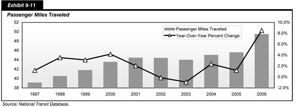
From 1997 to 2006, annual transit PMT increased from 39.2 billion to 49.5 billion, growing at an average annual rate of 2.6 percent. Annual change in transit travel over the 10-year period, as shown in Exhibit 9-11, was not consistent, ranging from a low of -0.9 percent in 2003 to a high of 8.5 percent in 2006. The variance in PMT rates of change can be attributed to a variety of factors, including the strength of the U.S. economy, the prevalence of public transportation, and the price of gasoline.
Transit Travel Growth Forecasts
Forecasting demand for public transportation services is an inexact science. The growth rate forecasts used by TERM are provided by MPOs, regional planning authorities comprising representatives from local governments, regional and State transportation authorities, and other civic organizations. It is not uncommon for long-range demand forecasts to deviate from actual growth in demand for transit services.
This section of Chapter 9 describes how recent observed changes in PMT have diverged from the long-range demand forecasts used by TERM. Beginning with a discussion of how PMT are changing in all urbanized areas, the section moves to explore rates of change in PMT in the investment scenarios described in Chapters 7 and 8. [It is important to note that to calculate PMT for the periods shown in Exhibit 9-11 through Exhibit 9-15 (e.g., January 2007 to June 2008), the FTA multiplied current monthly unlinked trip data by 2006 average trip length data, which are the most recent data available.]
Exhibit 9-12 shows how the change in annual PMT for all urbanized areas in 2007 and 2008 has diverged from the average long-range transportation growth forecast used by TERM. The exhibit depicts the year-over-year percent change in PMT, showing, for example, that PMT grew 1.5 percent from January 2006 to January 2007. Note that PMT grew more rapidly than forecast in 11 of the 18 periods displayed in the exhibit. The horizontal line shows the annual growth forecast used by TERM (1.5 percent).
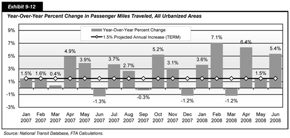
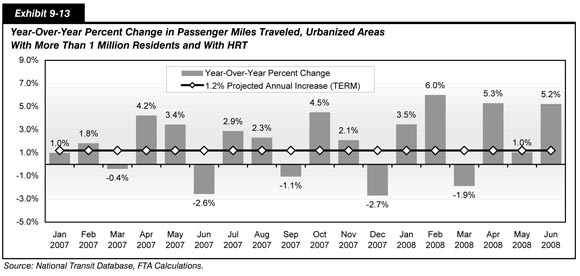
Exhibit 9-13 shows the annual rate of change in PMT for transit agencies operating in large metropolitan areas with heavy rail transit systems. The horizontal line in the exhibit represents the projected annual increase in boardings used by TERM for these urbanized areas. Annual rates of change observed in 2007 and early 2008 ranged from -2.7 percent to 6.0 percent. At 1.2 percent, the growth forecast utilized by the model is less than the annual change in PMT experienced by transit agencies in 11 of the 18 periods observed.
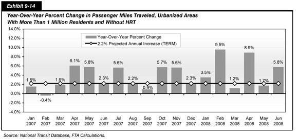
As shown by the horizontal line in Exhibit 9-14, the demand for public transportation services in large cities without existing heavy rail systems is expected to increase at an annual rate of 2.2 percent. This estimate is used by TERM to make its investment projections, as discussed in Chapters 7 and 8. With the exception of February 2007, when PMT decreased by -0.4 percent when compared with a year earlier, Exhibit 9-14 shows that PMT increased rapidly in 2007 and the beginning of 2008, growing at annual rates ranging from 0.9 percent to 9.5 percent. This suggests that current projections are underestimating the growth in demand for transit services in these metropolitan areas.
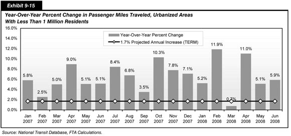
Small cities and rural areas experienced relatively high levels of PMT growth in 2007 and early 2008, surpassing the rate of change used by TERM in 17 of the 18 periods shown in Exhibit 9-15. Growth in PMT, measured on an annual basis, ranged from 0.7 percent to 11.9 percent over the 18-month period.
Projected and Historical Transit Travel Growth
TERM's projections of investments required to support the projected, natural growth in transit ridership are driven entirely by ridership and PMT forecasts provided by a sample of the Nation's MPOs. This sample is dominated by the Nation's largest urbanized areas (which are well represented) but also includes a mix of small- and medium-sized metropolitan areas from around the Nation. This section compares the 1.5 percent, weighted-average projected annual growth in PMT derived from these MPO projections (for the 2006 to 2026 forecast period), with the actual rate of growth in transit passenger miles as reported by the Nation's local transit agencies to the National Transit Database. This comparison suggests that the rate of growth projected by the MPOs (in aggregate) for the upcoming 20 years is less than that experienced nationally over the past decade. Should transit PMT continue to increase at rates closer to the recent historical rates (i.e., higher than the MPO projections), then the expansion (or maintain performance) needs estimates presented in Chapter 8 are less than will be required to maintain performance at today's levels.
Exhibit 9-16 presents the actual and MPO projected annual national growth rates for PMT for the period 1991 through 2026. Actual PMT data are presented for 1991 to 2007, with 2008 represented by 6 months of actual data and 6 months of forecast data. From 2009 through 2026, the exhibit presents the rate of increase of 1.5 percent derived from the MPO forecasts.
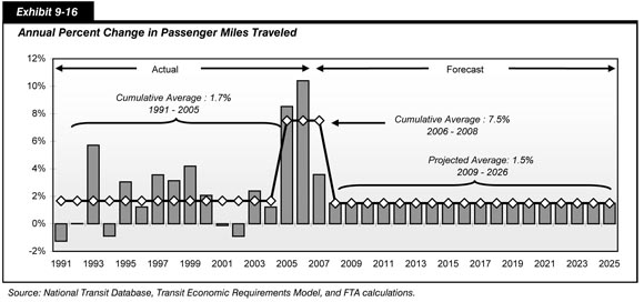
As shown in the exhibit, the period 1991 through 2005 was characterized by wide variations in PMT growth. While growth was positive in most of these years, total PMT did contract in 1992, 1995, 2002, and 2003. The average rate of PMT growth for the entire period was 1.7 percent. The PMT data for 2006, 2007, and the first 6 months of 2008 are characterized by significantly higher growth rates (averaging 7.5 percent) as compared with the prior period, driven primarily by the recent increases in fuel prices and the resulting shift from automobile travel to transit (and which may be a one-time increase). When evaluated from 1991 through the first 6 months of 2008 (to date), the average rate of PMT growth is 2.7 percent. Hence, regardless of the period over which the historical PMT growth is evaluated (i.e., over the 1991 to 2006 period or over the 1991 to 2008 period that includes the recent jump in transit ridership), the historical rate of increase exceeds the rate based on MPO projections. Once again, if the actual rate of increase over the next 20 years more closely reflects recent historical growth than the MPO projected rate of growth, then the needs estimates for asset expansion presented in Chapter 8 would be insufficient to maintain current transit performance into the future.
Commodity Inflation
The transit investment estimates described in Chapters 7 and 8 are presented in constant 2006 dollars and consequently do not capture any increases in prices from that time forward. At the same time, prices for materials and labor used in the construction industry have increased significantly in recent years, pushing the costs for constructing all types of capital projects upward. Most of this recent accelerated increase in construction and related materials inflation is not captured by the current TERM analysis.
Exhibit 9-17 presents the annual change in national construction costs since 1960. The vertical bars in the exhibit, measured on the left scale, are index numbers, while the line, measured on the right scale, represents the percent change in the index from year to year. While not fully representative of the materials and labor types used in transit capital projects (no index currently exists for transit capital projects), the index presented here is representative of construction costs in general. Following a period of high cost inflation from the late 1970s and early 1980s, cost growth moderated over the period from 1984 through 2003, ranging from 0.7 percent to 4.2 percent. In 2004, however, prices for construction goods and services began to rise at a more rapid pace, with year-over-year inflation reaching 8.9 percent before moderating to 4.3 percent in 2007. Much of this increase is driven by increases in the price of concrete, steel, and other key materials used in major transit capital projects.
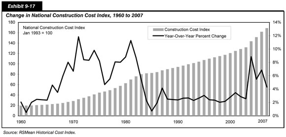
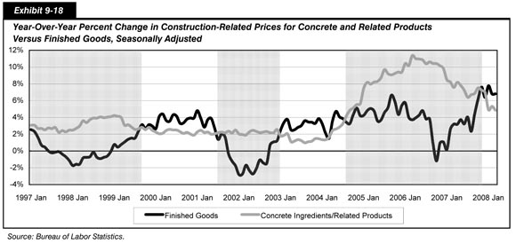
Exhibit 9-18 displays the annual percent change in the price of concrete ingredients and related products. These increases are compared to the annual percent change in the price of finished goods, a frequent measure of inflation for goods purchased by private sector producers in the United States. Shaded areas on the exhibit highlight periods of time when the rate of inflation for concrete ingredients and related products has exceeded that of finished goods. The data show that inflation for concrete products reached a peak in 2006, rising 11.4 percent from March 2005 to March 2006. While the pace has abated somewhat since 2005, price increases remains high by recent historical standards.
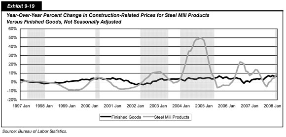
Steel is another major component in major transit capital projects, where it is used in the construction of new trackwork, elevated structures, bridges, facilities, and transit vehicles. Similar to other commodities used in the construction industry, the recent rate of increase in steel prices is high by historical standards. Exhibit 9-19 displays the rate of price inflation for steel mill products over the past 10 years, compared with the price of finished goods. Once again, time periods where the increase in the steel prices outpaced the increase in finished goods prices are highlighted by shaded areas. Note that the price of steel rose rapidly in the period from 2003 to 2004, increasing by as much as 49.7 percent in the 12 months leading to November 2004, before decreasing by 6.2 percent in the 12 months leading to August 2005. Inflation also accelerated in 2006, when prices increased by 22.7 percent from August 2005 to August 2006.
Once again, the current TERM projections do not fully capture these recent increases in the rate of cost inflation for key transit capital inputs. This is primarily due to the absence of a transit-specific capital cost index.
Comparison
The layout and content of Part II of this edition of the C&P report, including Chapters 7 through 10, has been restructured significantly relative to that of recent editions. Some of the material presented in this chapter builds on analyses presented in Chapter 9 of the 2006 C&P Report, but this edition also adds a series of new analyses that address some additional key issues relating to relationships between capital investment and the conditions and performance of the transportation system. This information is provided to assist in the interpretation of the selected future capital investment scenarios presented in Chapter 8, and to tie together the historic financial information presented in Chapter 6 with the conditions and performance information presented in Chapters 3 and 4.
Exhibit 9-20 provides a crosswalk between the information presented in the exhibits located earlier in this chapter, and the location of comparable information in the 2006 C&P Report.
| Chapter 9 Exhibit | Location of Comparable Information in the 2006 C&P Report |
|---|---|
| Exhibit 9-1 | Comparable to information shown in Exhibit 9-5. |
| Exhibit 9-2 | Comparable to information shown in Exhibit 9-6. |
| Exhibit 9-3 | No direct equivalent. |
| Exhibit 9-4 | No direct equivalent. A discussion of investment timing in HERS was included in Chapter 10. |
| Exhibit 9-5 | No direct equivalent. A discussion of investment timing in HERS was included in Chapter 10. |
| Exhibit 9-6 | No direct equivalent. |
| Exhibit 9-7 | No direct equivalent. |
| Exhibit 9-8 | No direct equivalent. |
| Exhibit 9-9 | No direct equivalent. |
| Exhibit 9-10 | No direct equivalent. |
| Exhibit 9-11 | No direct equivalent. |
| Exhibit 9-12 | No direct equivalent. |
| Exhibit 9-13 | No direct equivalent. |
| Exhibit 9-14 | No direct equivalent. |
| Exhibit 9-15 | No direct equivalent. |
| Exhibit 9-16 | No direct equivalent. |
| Exhibit 9-17 | No direct equivalent. |
| Exhibit 9-18 | No direct equivalent. |
| Exhibit 9-19 | No direct equivalent. |
Highways and Bridges
The highway section of this chapter retains two key elements from Chapter 9 in the 2006 C&P Report: (1) a discussion of the linkages among recent trends in system conditions, system performance, and capital spending, relative to what might have been expected based on the findings of the selected capital investment scenarios; and (2) a discussion of historic and projected future travel growth. Exhibits 9-1 and 9-2 are directly comparable to exhibits in Chapter 9 of the 2006 C&P Report depicting past and projected future highway vehicle miles traveled (VMT).
This section includes new elements, including discussions of inflation, the timing of investment, and the timing of congestion topics. Exhibit 9-3 illustrates how the constant dollar figures presented in this report could be converted to nominal dollars; previous C&P reports did not include this type of example. Exhibits 9-4 through 9-7 describe the system performance implications of alternative assumptions about the timing of capital investments; the discussion relating to these exhibits draws in material on the existing backlog of cost-beneficial highway capital investments and investment timing that was included in Chapters 7 and 10, respectively, in the 2006 C&P Report. Exhibit 9-8 discusses the implications of alternative assumptions regarding the timing of the widespread adoption of congestion pricing strategies; this topic was not addressed in the 2006 C&P Report.
Transit
For the transit section of this chapter, several new discussions have been added to the future impacts discussions. Future impact scenarios, which now compose the main content of this chapter, include the traditional ridership response to investment, as well as the added impact of congestion pricing on CO2 emissions; a comparison of the growth rates of passenger miles traveled (PMT) used by TERM's asset expansion module with the recent, actual PMT growth rates; and a discussion on recent construction commodity price inflation. Exhibits 9-9 and 9-10 focus on the assumptions driving the transition of VMT to PMT when highway users are diverted to transit and the impact of this diversion on rail and nonrail PMT. The key element of this analysis is the estimated reduction in CO2 emissions. Exhibits 9-11 through 9-16 focus on a detailed discussion of historic PMT growth rates through 2006, actual PMT between 2006 and 2008 which are significantly higher than historic and projected levels of growth, and the projections driven by data collected from metropolitan planning organizations. Exhibits 9-17 through 9-19 present recent trends in construction cost indices that would impact transit capital projects. These are important to note because the majority of this recent inflationary trend in construction and related materials is not currently captured within TERM. A discussion of current impacts on physical conditions and operational performance has been removed from Chapter 9, but is included in detail in Chapters 7 and 8.