U.S. Department of Transportation
Federal Highway Administration
1200 New Jersey Avenue, SE
Washington, DC 20590
202-366-4000
This chapter describes the various highway-related costs considered in this study and provides estimates of those costs for the ISTEA base period (1993-1995) and the 2000 analysis year. Previous Federal HCASs have focused primarily on allocating actual or anticipated highway improvement costs paid from the HTF, including costs of providing new highway capacity, preserving the physical condition of the highway system, safety improvements, TSM, environmental enhancement, and other improvements. State HCASs also have focused on allocating highway-related costs paid from HURs, because, like the Federal studies, they have been primarily interested in questions of whether highway user fees are being levied among different groups of users in proportion to their share of highway cost responsibility.
The HCASs historically have allocated either actual or anticipated expenditures/obligations by highway agencies. They have not allocated amounts that should be spent to maintain system condition, reduce congestion, or achieve other broad policy objectives. While this might be useful information if some change in either highway program level or composition were being considered, most HCASs have focused on the specific question of how much of actual or planned program costs should be paid by different vehicle classes?
Allocating infrastructure and other costs paid from the Federal HTF continues to be a key focus of the current Federal HCAS, but a number of costs that have not been treated extensively in previous Federal cost allocation studies are examined in this study. For instance, costs for pedestrian and bicycle facilities, mass transit improvements, and enhancements that have become increasingly important since passage of ISTEA were not included in the 1982 Federal HCAS, but are included in this study.
Federal costs paid from the HTF are estimated primarily from the FMIS which contains data on obligations of Federal funds and State matching funds by improvement type and highway functional class for projects constructed through the Federal-aid highway program. The FMIS data are supplemented with information from other sources on key components of construction projects that are not available from the FMIS.
This study also evaluates highway-related costs such as air pollution, noise, global warming, and community disruption that are borne by the general public rather than by highway users or highway agencies. There is increasing concern that failure to consider such costs in investment and other infrastructure management decisions may lead to inefficient resource allocation and may unfairly subsidize users of one mode over another. Regulatory programs have been successful in reducing some external costs, notably air pollution and crash costs, and significant HURs are spent on programs such as transportation demand management, safety improvements, CMAQ improvement, noise barrier construction, and beautification to mitigate external highway costs. The responsibility of different vehicle classes for these external costs is estimated and compared to cost responsibilities for agency costs as a further indicator of highway user fee equity. This information also provides a framework for evaluating additional actions that can be taken to reduce external costs.
One approach advocated by some to reduce external costs is to charge highway users for either the full or marginal costs of their trips, including congestion, air pollution, and other external costs they impose on others as a result of their travel decisions. Only those users who value their trips at least as much as the cost of those trips, including costs imposed on others, would travel during periods when congestion and other external costs were high. Some users would decide not to make a trip, others would change either the time or destination of the trip to avoid paying the highest tolls, and still others would switch to alternative modes that have lower costs. Congestion, air pollution and other external costs thus would be reduced, and users who continue to travel during times when external costs are high would generate substantial revenues for transportation agencies.
True congestion pricing has never been applied by transportation agencies in this country, although a private toll road in California has instituted variable tolls by time of day, and a project is underway in San Diego under the Congestion Pricing Pilot Program that will have tolls which vary according to the level of congestion. Other areas are evaluating the feasibility of variable pricing under the Congestion Pricing Pilot Program. Peak period pricing is common in other sectors of the economy. Utilities, phone companies, theaters, restaurants, and other businesses routinely charge more during peak periods to ration demand and maximize profits. Forms of congestion pricing have been applied on a very limited scale to highway transportation in several foreign countries. An example of charges being levied to reduce transportation-related externalities in the United States is the "gas guzzler" tax imposed on vehicles that do not achieve a minimum fuel economy standard.
External costs were discussed in an appendix to the 1982 Federal HCAS in which marginal highway costs, including environmental and congestion costs, were examined to estimate economically efficient user fee rates that would have to be charged for different vehicles operating under different conditions. A comprehensive treatment of external costs of highways is beyond the scope of this study, but Chapter V examines key external costs of highway use and operation as they pertain to evaluating the equity and efficiency of highway user charges. In addition to estimating marginal costs under different conditions, total external costs attributable to different vehicle classes are estimated. While there is considerable uncertainty surrounding estimates of these external costs, their magnitude makes it essential to consider these costs in highway policy studies.
Just as the broader costs of highway use have received increasing attention recently, so too have the broader economic benefits of highways, especially benefits to industry productivity and international competitiveness. During the course of this study there was considerable discussion concerning the treatment of highway benefits. Much of the discussion revolved around the issue of whether there are external benefits of highway use comparable to external costs of highway use. The consensus among most economists was that there are few if any truly external benefits associated with the use of the highway. Almost all commercial benefits associated with highway use represent transfers of benefits realized by highway users, and to include those benefits along with benefits to highway users would result in double-counting. There was general agreement, however, that there are substantial public and private benefits of highways over and above savings in travel time and vehicle operating costs realized by highway users. Estimating the magnitude of those benefits was outside the scope of this study, however. Appendix D summarizes relationships between highway user benefits and costs and results of recent FHWA research on relationships between highways and economic productivity. Other benefits such as the contribution of highway programs to sustainable redevelopment and brownfields redevelopment are not discussed in this report, but these clearly are examples of how targeted and coordinated highway investment can contribute to a variety of local social and economic development objectives. The Department's biennial C&P Report presents results of extensive analyses of benefits of alternative investment levels in surface transportation programs and demonstrates the significant benefits of highway investment.
 Base
Period HighwayProgram Costs
Base
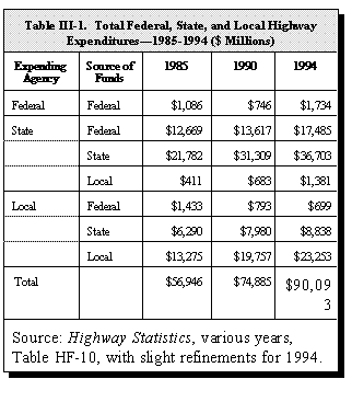
Period HighwayProgram CostsTable III-1 shows trends in total expenditures for highways by all levels of government. Since substantial amounts are transferred among different levels of government, sources of funds are also shown. Funds for mass transit programs are not included in this table although they are included in subsequent analyses of Federal costs. Highway construction and maintenance activities by Federal agencies in national parks, forests, and other Federal lands constitute the largest share of direct Federal expenditures for surface transportation. Direct Federal highway expenditures represent 9 percent of total highway expenditures from Federal funds. The bulk of Federal HURs are paid to States as reimbursements for the Federal share of project costs under the Federal-aid highway program.
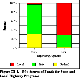
State and local shares of total highway expenditures have remained fairly stable over the period at about 61 percent and 37 percent, respectively. Federal funds currently constitute about 31 percent of total funding for State highway construction programs. Relatively little Federal money goes into local highway programs, but substantial amounts of State HURs are transferred to county and municipal governments to finance local highway programs. Figure III-1 shows the sources of funds for 1994 State and local highway programs.
 Federal highway
program cost data were extracted and analyzed from FHWA's FMIS. The FMIS
is a formal, interactive, on-line database which provides detailed information
on Federal-aid highway projects. Project-related information originates at the State
departments of transportation, but is entered in the FMIS by FHWA staff. The FMIS
represents the best source of project-related information for Federal-aid highway
projects, and was analyzed in detail to provide insight on the use of Federal highway
program funds. The FMIS includes information on obligations of Federal and State matching
funds for Federal-aid projects, not on actual expenditures. Funds are obligated when
specific obligation authority is attached to a project. Adjustments to obligated funds are
made as the project progresses through various stages of completion. Project expenditures
do not necessarily occur at the same time as obligations, and obligations for a project in
1 year may result in actual expenditures over more than 1 year.
Federal highway
program cost data were extracted and analyzed from FHWA's FMIS. The FMIS
is a formal, interactive, on-line database which provides detailed information
on Federal-aid highway projects. Project-related information originates at the State
departments of transportation, but is entered in the FMIS by FHWA staff. The FMIS
represents the best source of project-related information for Federal-aid highway
projects, and was analyzed in detail to provide insight on the use of Federal highway
program funds. The FMIS includes information on obligations of Federal and State matching
funds for Federal-aid projects, not on actual expenditures. Funds are obligated when
specific obligation authority is attached to a project. Adjustments to obligated funds are
made as the project progresses through various stages of completion. Project expenditures
do not necessarily occur at the same time as obligations, and obligations for a project in
1 year may result in actual expenditures over more than 1 year.
In addition to obligation data, the FMIS contains additional project-related data that are useful to analyze project costs. For example, there are FMIS fields that contain information for each project on State, urbanized area, county, urban/rural, highway type, improvement type, work class, bridges, pavements, safety type, and work type. Given the number of projects contained in the FMIS, extracting and organizing this information is a substantial task. For this study, Federal highway obligations data were primarily collected and reported by improvement type (e.g., new capacity, major widening) and highway functional class (e.g., Urban Interstate, Rural Interstate). However, further detailed information was available on individual work types and this data was extracted and incorporated to ensure appropriate vehicle class attribution. For example, numerous queries were made to separately quantify Federal obligations for truck-related expenditures, such as truck scales, loading facilities, terminal and transfer facilities, and various truck safety programs.
The distribution of Federal highway obligations by improvement type and highway
functional class varies from year to year for several reasons including distortions caused
by major projects obligated during a year, emphasis on a particular type of improvement by
States during the year, or other reasons. To minimize annual variations in patterns of
obligations and to present a more accurate picture of the composition of the current
program under ISTEA, Federal obligations are averaged for the Years 1993, 1994, and 1995
to represent the ISTEA base period.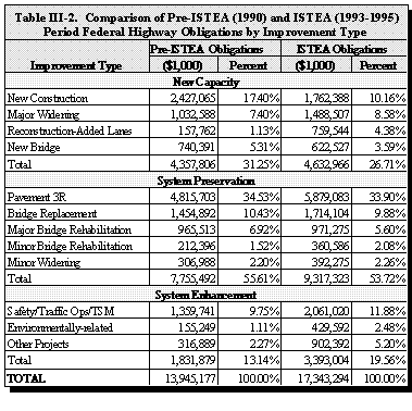
Table III-2 compares obligations of Federal highway funds in 1990 with the ISTEA (1993-1995) base period. The composition of Federal obligations for highways has changed since passage of ISTEA in 1991. Approximately the same percentage of Federal obligations went for system preservation in the ISTEA period as prior to ISTEA, but the percentage of funds obligated for new capacity declined by about five percentage points while the percentage for system enhancements increased by five percentage points. This reflects the emphasis on enhancements in ISTEA and increased reliance on alternatives to constructing new highway lanes to improve traffic operations and reduce congestion.
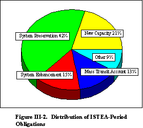
Figure III-2 summarizes the composition of Federal highway by improvement type in the ISTEA base period (1993-1995). Over 20 percent of obligations were for added capacity, 42 percent for system preservation, 15 percent for system enhancement, 13 percent for mass transit improvements financed from the MTA of the HTF, and 9 percent for other purposes, including improvements on Federal lands and FHWA administrative expenses. This table does not include obligations for transit improvements and certain other miscellaneous costs, but shows trends in obligations for key highway improvement types.
 In the ISTEA base
period, adding highway lanes, either on new location (new construction)
or to existing highways (major widening and reconstruction with added lanes)
represented over 85 percent of total new capacity costs. New bridges represented less
than 15 percent of new capacity costs. Likewise, system preservation costs are dominated
by costs to reconstruct, rehabilitate, or resurface pavements. Almost two-thirds of
system preservation costs are for pavement improvements compared to about one-third
for bridge improvements. System enhancement costs represent remaining costs under the
Federal-aid highway program that are neither for new lanes, new bridges, nor preservation
of existing pavements and bridges. These costs include costs for safety improvements, TSM,
environmental enhancements, transit improvements funded from the Highway Account of the
HTF, and other costs. Costs for mass transit funded from the MTA of the HTF are shown
separately from transit costs funded from the Highway Account to emphasize the fact that
these funds generally do not flow through State transportation agencies in the same manner
as transit projects funded from the Highway Account. Obligations from the MTA were
approximately 13 percent of total Federal highway-related obligations from the HTF in the
ISTEA base period. The remaining obligations from the HTF were for direct Federal
construction on Federal lands, contributions to National Highway Traffic Safety
Administration (NHTSA) safety programs, FHWA administration, and other miscellaneous
expenses altogether constituting about 9 percent of total HTF obligations.
In the ISTEA base
period, adding highway lanes, either on new location (new construction)
or to existing highways (major widening and reconstruction with added lanes)
represented over 85 percent of total new capacity costs. New bridges represented less
than 15 percent of new capacity costs. Likewise, system preservation costs are dominated
by costs to reconstruct, rehabilitate, or resurface pavements. Almost two-thirds of
system preservation costs are for pavement improvements compared to about one-third
for bridge improvements. System enhancement costs represent remaining costs under the
Federal-aid highway program that are neither for new lanes, new bridges, nor preservation
of existing pavements and bridges. These costs include costs for safety improvements, TSM,
environmental enhancements, transit improvements funded from the Highway Account of the
HTF, and other costs. Costs for mass transit funded from the MTA of the HTF are shown
separately from transit costs funded from the Highway Account to emphasize the fact that
these funds generally do not flow through State transportation agencies in the same manner
as transit projects funded from the Highway Account. Obligations from the MTA were
approximately 13 percent of total Federal highway-related obligations from the HTF in the
ISTEA base period. The remaining obligations from the HTF were for direct Federal
construction on Federal lands, contributions to National Highway Traffic Safety
Administration (NHTSA) safety programs, FHWA administration, and other miscellaneous
expenses altogether constituting about 9 percent of total HTF obligations.
The detailed data available in the FMIS include the functional highway class upon which improvements are made. Disaggregation of improvement costs by highway functional class allows differences in traffic composition, highway design, and other factors that vary by highway type to be fully considered in estimating the cost responsibility of different vehicle classes.
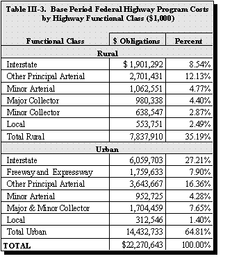 Table III-3 shows
the distribution of ISTEA base period Federal obligations by highway functional class.
Thirty-five percent of total obligations are on rural highways and 65 percent on
urban highways. Over half of all obligations on rural roads are on higher order systems
(Interstate or other principal arterial highways) and three-quarters of urban obligations
are on higher order systems (Interstate highways, other freeways and expressways, and
other principal arterial highways). Other factors being equal, vehicle classes with
greater shares of travel on higher order systems will have relatively greater cost
responsibilities than vehicles traveling predominantly on lower order systems because so
much of the money is spent on higher-order systems.
Table III-3 shows
the distribution of ISTEA base period Federal obligations by highway functional class.
Thirty-five percent of total obligations are on rural highways and 65 percent on
urban highways. Over half of all obligations on rural roads are on higher order systems
(Interstate or other principal arterial highways) and three-quarters of urban obligations
are on higher order systems (Interstate highways, other freeways and expressways, and
other principal arterial highways). Other factors being equal, vehicle classes with
greater shares of travel on higher order systems will have relatively greater cost
responsibilities than vehicles traveling predominantly on lower order systems because so
much of the money is spent on higher-order systems.
Figure III-3 summarizes the distribution of highway improvements on different
functional highway classes. There are substantially more capacity improvements on
high-order systems than on lower order systems. The proportion of obligations for new
capacity on high-order urban systems is more than twice as great as on low-order systems
in either rural or urban areas. Relatively more is spent on system preservation on rural
highways than urban highways, especially low-order rural highways where system
preservation accounts for over two-thirds of total obligations. System enhancements
including safety improvements, TSM, transit improvements, and various other enhancement
projects account for 40 percent of obligations on low-order urban highways, a
substantially greater share than on other highway systems.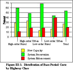
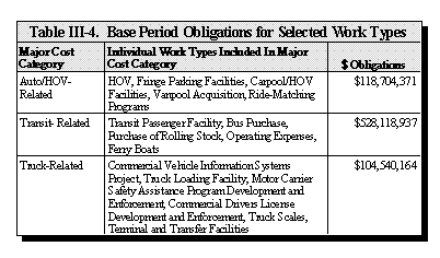
The FMIS contains more detailed data on specific types of highway improvements than were available for the 1982 Federal HCAS. The most detailed information in FMIS is the project work type. Detailed data on work types provides the basis for a more accurate assignment of highway cost responsibility among different vehicle classes because many different types of work may be included in a single broad improvement type. Detailed work type data help to assure that costs are not incorrectly attributed to the wrong vehicle class and allow some costs that otherwise might simply be lumped with common costs to be identified and allocated to particular vehicle classes. Table III-4 summarizes obligations for work types used in this study categorized by the nature of the work. Table III-5 shows the distribution of Federal obligations for 12 highway improvement types into which Federal-aid highway program obligations are grouped. Obligations for each improvement type are distributed across the 12 highway functional classes.
 The potential for
more widespread use of LCCA to reduce overall system preservation costs was evaluated on a
preliminary basis in this study. The LCCA of infrastructure investment decisions is
intended to identify alternatives that have the lowest cost over their entire life, not
just alternatives with the lowest initial costs. Among the factors that can affect life
cycle costs are the materials selected for particular types of construction, the
initial design, and maintenance and rehabilitation (M&R) practices. Many States
apply LCCA principles to varying degrees in pavement and bridge management systems, but
there is a widespread belief that greater use of LCCA could reduce long-term program
costs. The implications of LCCA for HCA are that if long-term infrastructure costs could
be reduced, those costs would represent a smaller share of the overall program and vehicle
classes responsible for the greatest share of infrastructure costs would have lower cost
responsibility and improved equity ratios.
The potential for
more widespread use of LCCA to reduce overall system preservation costs was evaluated on a
preliminary basis in this study. The LCCA of infrastructure investment decisions is
intended to identify alternatives that have the lowest cost over their entire life, not
just alternatives with the lowest initial costs. Among the factors that can affect life
cycle costs are the materials selected for particular types of construction, the
initial design, and maintenance and rehabilitation (M&R) practices. Many States
apply LCCA principles to varying degrees in pavement and bridge management systems, but
there is a widespread belief that greater use of LCCA could reduce long-term program
costs. The implications of LCCA for HCA are that if long-term infrastructure costs could
be reduced, those costs would represent a smaller share of the overall program and vehicle
classes responsible for the greatest share of infrastructure costs would have lower cost
responsibility and improved equity ratios.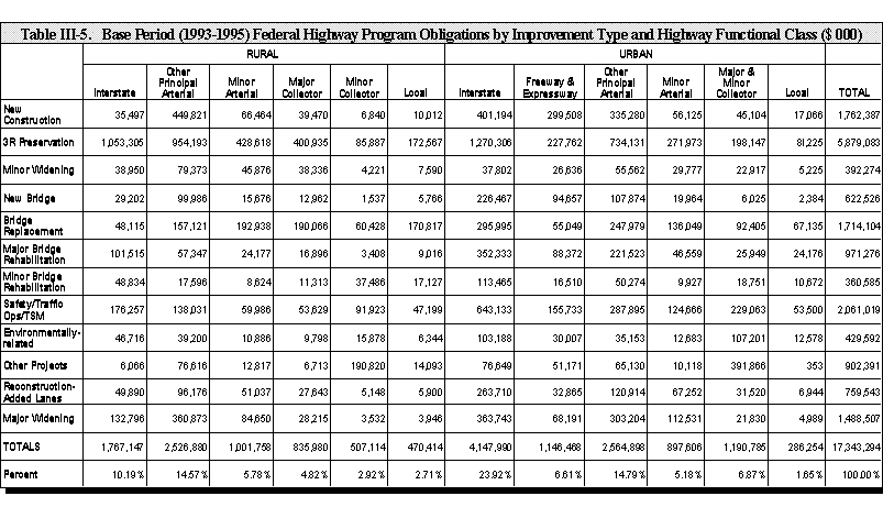 The NHS Designation Act of 1995 (P.L. 104-59, 109 Stat. 568 (1995))
requires the use of LCCA on NHS projects having a usable project segment costing $25
million or more. The FHWA recently issued a final policy statement on LCCA implementing
LCCA provisions of this Act and generally encouraging the use of LCCA in evaluating major
infrastructure investment decisions.
The NHS Designation Act of 1995 (P.L. 104-59, 109 Stat. 568 (1995))
requires the use of LCCA on NHS projects having a usable project segment costing $25
million or more. The FHWA recently issued a final policy statement on LCCA implementing
LCCA provisions of this Act and generally encouraging the use of LCCA in evaluating major
infrastructure investment decisions.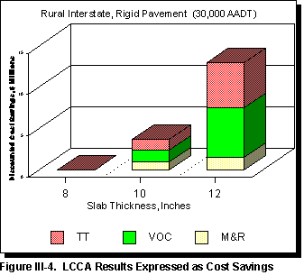
A preliminary analysis suggests large potential benefits from the adoption of LCCA, especially in reducing vehicle operating costs associated with traveling on deteriorated pavements and delay around work zones where highway M&R is being performed. Typical life-cycle cost results are illustrated in Figure III-4, showing the variation in agency costs (M&R combined), vehicle operating costs (VOC), travel time costs, and total costs (agency plus user) as a function of pavement structure assuming a given traffic level. The specific example shown in Figure III-4 applies to rural Interstate highways with 30,000 annual average daily traffic (AADT), and rigid pavement structures ranging from a slab thickness of 8 to 12 inches. These costs were obtained by simulating the performance of the indicated pavement structures under a traffic load of 30,000 AADT, comprising a mix of vehicles estimated for this functional class.
An analysis period of 50 years was used, and costs were discounted at 4 percent. While these results in Figure III-4 apply to the specific case described, they typify the results seen in other cases in the following ways:
To determine whether rehabilitation policies approach an optimal or least cost pavement
strategy, analyses were made of a given pavement and traffic situation (flexible pavement,
structural number of 5.0, carrying 50,000 vehicles per day). Figure III-5 shows cost
savings, primarily in vehicle operating costs, associated with rehabilitating pavements
before pavement condition, as measured by the pavement serviceability index (PSI) gets too
poor. The additional M&R costs of these policies, shown as negative cost savings, are
the agency costs to perform more rehabilitation. The analysis conducted for this study did
not examine options of allowing pavement to deteriorate below a PSI of 2.5, but in some
case agency cost savings might be expected from policies that prevented pavements from
deteriorating to the point where they needed major reconstruction. The cost savings with
each successively higher PSI occur in both vehicle operating costs and travel time
costs, according to the EAROMAR model. It is instructive to note, however, that while
savings in travel time costs increase in the steps from threshold values of 2.5 to 3.0 and
from 3.0 to 3.5, no such gain occurs from a threshold of 3.5 to 4.0. Two effects
contribute to this situation: (1) in the range of PSI from 3.5 to the maximum
theoretical PSI of 5.0, the pavement is so smooth that little additional speed is gained
as a function of further improvements in pavement surface condition; and (2) the
additional congestion costs due to more frequent pavement rehabilitation and the
imposition of work zones detract from any travel time savings due to incrementally
smoother pavement. The gains in vehicle operating costs at all levels of improvement in
rehabilitation policy can be substantial according to the results in Figure III-5. Further
research to improve estimates of potential benefits of LCCA is planned, not only for cost
allocation but for investment analyses conducted for the Department's C&P Report.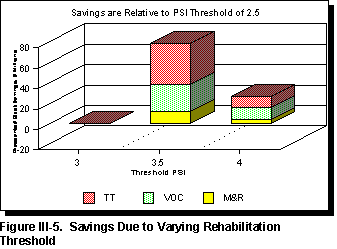
Federal obligations for transit are highlighted in Table III-6. About three-fourths of the total Federal funds for mass transit are from the HTF. About 15 percent of trust fund monies for mass transit are from the Highway Account and 85 percent from the MTA. Of those HTF funds, almost all are for capital outlays.
The Federal Transit Administration (FTA) groups transit expenditures into three broad
functions, congestion management, low-cost mobility, and liveable metropolitan areas.
These functions are not mutually exclusive, however, and thus the amount that is
exclusively for any one function cannot be estimated. Expenditures for congestion
management represent the largest share of total transit expenditures, and total estimated
expenditures related to congestion management exceed monies obligated for transit from the
HTF. In allocating transit costs, it is assumed that all monies from the HTF are related
to congestion management, and thus can appropriately be allocated to highway users.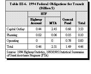
There is considerable uncertainty about the future composition and funding level for the Federal highway program. Significant changes in Federal surface transportation programs were enacted in ISTEA which provide unprecedented flexibility for State and local transportation agencies to meet their unique transportation requirements while focusing resources on a new NHS that will be the backbone of surface transportation systems into the next century. This flexibility has been widely heralded, but some believe there is too much flexibility, while others believe there should be even more. Similarly there is much debate concerning the future level of Federal highway funding. Current budgetary limitations have required all Federal agencies to reassess priorities and make do with less funding in many cases.
In the current budgetary environment, it is difficult to predict what the Federal highway program composition and funding level will be in 2000, the forecast year for this study. For purposes of simplifying the analysis, the composition of the highway program in 2000 is assumed to be the same as during the 1993-1995 base period. The distribution of obligations by improvement type is assumed to be the same as well as the distribution across highway functional classes. Furthermore, the program level is assumed to be the same as revenues coming into the HTF. Actual obligation levels are determined by Congress and could be below, equal to, or above HTF revenues.
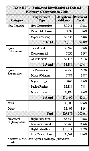 These assumptions
have significant implications for the equity analysis because both the distribution of
obligations by improvement type and highway class influence the allocation of program
costs among different vehicle classes. Table III-7 shows the assumed distribution of
obligations from the HTF in 2000. Because the composition of the Federal program can have
such a large impact on the equity analysis, alternative investment scenarios are evaluated
in Chapter VI. These scenarios consider a wide range of potential options including
greater investment in system preservation, greater investment in added capacity, and
greater investment in system enhancement.
These assumptions
have significant implications for the equity analysis because both the distribution of
obligations by improvement type and highway class influence the allocation of program
costs among different vehicle classes. Table III-7 shows the assumed distribution of
obligations from the HTF in 2000. Because the composition of the Federal program can have
such a large impact on the equity analysis, alternative investment scenarios are evaluated
in Chapter VI. These scenarios consider a wide range of potential options including
greater investment in system preservation, greater investment in added capacity, and
greater investment in system enhancement.
Unlike the detailed data on Federal obligations for highway construction, detailed descriptions of State and local obligations for highway construction and maintenance are not available. As a result, data on State and local highway costs are developed on an expenditure basis. There is no database that provides detailed information on expenditures by specific improvement or work types or by highway functional class as is the case for Federal program costs. Thus, data at a more general level must be used for the analysis. (See Appendix H, "Highway Cost Allocation for All Levels of Government" for more details on State and local expenditures.)
The largest single category of highway expenditures for all levels of government is capital outlay, followed by maintenance services. As explained previously, capital outlays are those costs associated with the planning, engineering, and construction of improvement projects, while maintenance expenditures preserve existing facilities. All other highway-related expenditures by State and local governments have been grouped into other costs. There do not appear to be any consistent changes in types of highway expenditures from year to year, but rather small fluctuations.
The forecast of State and local highway expenditures is based on the future demand for highway transportation and the trends in State and local expenditures per VMT. Although highway expenditures have increased steadily over the past few decades, there has been a decline in total expenditures per VMT measured in constant dollars. This reduction in expenditures per VMT is partially attributed to the declining emphasis on new road construction and the growing need to maintain existing roads.
The forecast of State and local highway expenditures is based on changing characteristics of motor vehicle travel and historical trends in expenditures per VMT. Average expenditures per VMT are calculated for different categories of State and local highway expenditures to incorporate changes in efficiency of building, maintaining, and administering highway programs. State capital outlays are divided into urban and rural areas in order to account for shifts of motor vehicle travel; however, the remaining State and local expenditures such as administration, safety, or law enforcement cannot be classified by type of roadway.
Capital outlays on rural roads averaged $9.24 per 1,000 VMT in 1994 and have decreased 1.6 percent annually since 1988. Capital outlays per 1,000 VMT on urban roads decreased 1.0 percent a year for the same period. On a per VMT basis, it is more costly to build and maintain rural roads than urban roads. This is attributed to the large initial cost of building roads and the lower marginal cost per vehicle mile of maintaining the roads. Administration and research is the only State expenditure category that has increased on a per VMT basis at 2.3 percent annually. Total State highway expenditures per VMT decreased 1.4 percent annually, with rural and urban capital outlays representing the largest decrease in spending per VMT.
Local highway expenditures per VMT decreased more significantly than State expenditures, led by declines in capital outlays, law enforcement/safety, and maintenance services. Capital outlays declined more than any other category at -3.54 percent per year (local capital outlays cannot be divided into rural and urban areas with the current data). Bond retirement and interest on debt are the only local costs to increase per VMT which indicates that local governments have been taking on larger debt to finance roadways. The total highway expenditures per VMT decreased at 2.4 percent per year, a full percentage point greater than State expenditures.
The forecast of State and local highway expenditures combines motor vehicle travel forecasts with the average change in expenditures per VMT to project total expenditure levels. This approach incorporates the historical trends in State and local spending for highways with the expected growth in motor vehicle transportation. Each category of State and local highway expenditures is projected in costs per VMT based on the compound annual growth rate for that category between 1988 to 1994. State capital outlays are divided into rural, urban, and unclassified expenditures and are projected separately (unclassified capital outlays are expenditures that have not been designated either rural or urban areas). Forecasted annual VMT is multiplied by the projected costs per VMT to calculate the future State and local annual highway expenditures.
 Table III-8
provides the estimates of growth rates for Federal, State, and local highway expenditures
for the various categories. All values are in millions of dollars and the growth rates are
compound annual rates projected from 1994 to 2000. Mass transit expenditures are projected
to increase the fastest at 5.76 percent, while maintenance expenditures and capital
outlays are projected to increase at 3.32 and 3.76, respectively. Other highway
costs, which include traffic services, administration and research, debt service, and law
enforcement are projected to grow at an overall rate of 5.56 percent. Total highway
expenditures are forecast to increase from $97.1 billion in 1994 to $125.3 billion in
2000, at an annual growth rate of 4.34 percent. Table III-8 provides a detailed breakdown
of expenditures for all levels of government and growth rates between 1994 and 2000.
Table III-8
provides the estimates of growth rates for Federal, State, and local highway expenditures
for the various categories. All values are in millions of dollars and the growth rates are
compound annual rates projected from 1994 to 2000. Mass transit expenditures are projected
to increase the fastest at 5.76 percent, while maintenance expenditures and capital
outlays are projected to increase at 3.32 and 3.76, respectively. Other highway
costs, which include traffic services, administration and research, debt service, and law
enforcement are projected to grow at an overall rate of 5.56 percent. Total highway
expenditures are forecast to increase from $97.1 billion in 1994 to $125.3 billion in
2000, at an annual growth rate of 4.34 percent. Table III-8 provides a detailed breakdown
of expenditures for all levels of government and growth rates between 1994 and 2000.
Expenditures by highway agencies do not cover all societal costs of highway construction and use. Use of the highway system can have unintended adverse impacts on other highway users and non-users. Among these adverse impacts are damage to health, vegetation, and materials due to air pollution; noise and vibration effects of traffic; congestion costs to other highway users; fatalities, injuries, and other costs due to crashes; and waste from scrapped vehicles, tires, and oil.
The construction of highways and their physical presence may also have unintended adverse impacts including environmental impacts during construction; aesthetic impacts on adjacent areas; effects of roadways as barriers to community interaction; water quality impacts such as loss of wetlands and run-off; and loss of parklands and wildlife habitats.
Legislation such as the National Environmental Policy Act (NEPA); Noise Control Act; National Historic Preservation Act; Clean Air Act and Amendments; Section 4(f) of the DOT Act; ISTEA; and legislation establishing NHTSA and funding safety improvements includes a number of important provisions designed to minimize adverse impacts associated with highway construction, highway use, motor vehicle characteristics, and other aspects of the transportation system. Minimizing the unintended costs of highway use and highway construction is a central consideration in transportation planning, programming, project design, and policy development. Another potential way to reduce congestion, environmental and other costs that highway users impose on others would be to charge users for those costs. Indeed, if users paid the marginal costs of their trips, economic efficiency would be improved. The marginal costs of highway use are the added costs associated with a unit increase in highway use (measured, for example, in cents per vehicle mile). These marginal costs include costs to the highway user (e.g., travel time and fuel), costs imposed on other highway users (principally crash costs and congestion) costs imposed on non-users, and costs borne by public agencies responsible for the highway system (e.g., use-related maintenance costs). Highway users take their own vehicle operating and travel time costs into account when they decide whether or not to make a trip, but they generally do not consider costs they impose on others.
Marginal costs are frequently characterized as "short-run" or "long-run." Short-run costs take the highway system as fixed. Long-run costs allow for the possibility of capital investment (e.g., construction of more lanes or thicker pavements) to accommodate increases in highway use. The basic goal of marginal cost pricing is improved economic efficiency: if highway users are required to pay fees equal to the costs they impose on others (including other highway users, non-users, and public agencies) when they choose to travel, then trips that are valued less than these costs will not be made. In congested urban areas, a substantial portion of the marginal costs of highway use are borne by other highway users and non-users. Marginal environmental, congestion, safety, and other social costs of travel by different vehicles are estimated in Chapter V. This chapter includes only total cost estimates for those various non-agency costs.
Several recent studies have advocated the use of full cost pricing of highways in assessing the equity of highway user tax structures. Full cost pricing of highways is based on the concept that highway user taxes should be set at levels that are sufficient to recover all costs of highway use, not just agency costs (as in a traditional application of the cost-occasioned approach) and not just short-run marginal costs (as in marginal cost pricing). In most past applications of full cost pricing, the primary focus has been on a comparison of total costs of the highway system with total collections from all highway users. However, if the responsibility for all costs can be allocated among vehicle classes, the results of a "full cost pricing" analysis can also be used as a basis for evaluating the relative shares of revenues from different vehicle classes. It is important to point out that environmental cost estimates developed in this report should not be used as a basis for calculating damages from specific infrastructure projects in affected areas.
Motor vehicles produce emissions that damage the quality of the environment and adversely affect the health of human and animal populations. Highway users are a major source of total air pollution in the United States. The EPA estimated that in 1993 approximately 62 percent of all carbon monoxide (CO) emissions, 32 percent of all nitrogen oxides (Nox), and 26 percent of volatile organic compounds were produced from highway sources. Air pollution generated from transportation vehicles is an external cost that is not fully absorbed by the transportation user. Environmental legislation requiring improved engine technology and cleaner burning fuels has internalized some of the emission damage caused by motor vehicles; however, the technological advances have not eliminated air quality damage from combustion engines.
Key motor vehicle characteristics affecting emission rates include the following:
The damage caused by pollutant emissions also varies greatly depending on meteorology, population, and other characteristics of the region in which the vehicle is operating. For a given vehicle, external costs for air pollution (expressed, for example, in dollars per vehicle mile) can vary by several orders of magnitude depending upon (1) the level of congestion under which travel occurs, sensitivity of nearby land uses, and other situational factors and (2) analysis assumptions such as those used to quantify effects of additional emissions on health.
Methods for estimating vehicle emission costs are divided into three primary components: the measurement of the emissions of a single vehicle operating under specific conditions, estimation of the emissions effect on ambient concentration levels, and the damage cost calculation for a unit change in concentration per person. Relating emission costs to changes in person-year concentration levels best captures the locational changes in ambient air quality and relates these conditions to the number of people affected by the pollutant. Unlike other key social costs, published studies did not provide an adequate basis for estimating the costs of air pollution attributable to highway use by motor vehicles. The Department is working with EPA to develop estimates that adequately reflect the lastest understanding of the costs of motor vehicle emissions. These cost will be submitted as an addendum to this report.
Noise emissions from motor vehicle traffic are a major source of annoyance, particularly in residential areas. Millions of people living near busy highways and roads are affected by vehicle traffic noise.
Key vehicle characteristics and situational factors affecting noise costs include the following:
Noise costs were estimated using information on the reduction in residential property values caused by noise emissions of highway vehicles. Estimates of noise emissions and noise levels at specified distances from the roadway were developed using FHWA noise models in which noise emissions vary as a function of vehicle type, weight, and speed. Data from FHWA's HPMS were used to estimate the types of development adjacent to highways for each highway functional class. Assumptions about residential densities for different types of development were then used to estimate the number of housing units affected. The procedures are described in Appendix E.
The following assumptions in Table III-9 were used to develop high, middle, and low estimates of noise costs:
| Table III-9. High, Middle, and Low Assumptions Used in Estimating Noise Costs | |||
| High | Middle | Low | |
| Percent change in value of residential property per decibel over threshold | 0.88 | 0.40 | 0.14 |
| Adjustment factor for other uncertainties in noise cost estimation | 1.2 | 1.0 | 0.8 |
 The 0.88 and 0.14
were the second highest and second lowest estimates from 17 noise impact studies conducted
from 1974 to 1980 and reviewed by Nelson (1982) (see Appendix E). It should be noted that
these costs were derived to estimate external costs and are not intended to be used for
assessing damage to developments adjacent to highways.
The 0.88 and 0.14
were the second highest and second lowest estimates from 17 noise impact studies conducted
from 1974 to 1980 and reviewed by Nelson (1982) (see Appendix E). It should be noted that
these costs were derived to estimate external costs and are not intended to be used for
assessing damage to developments adjacent to highways.
Table III-10 shows estimates of high, middle, and low estimates of noise costs developed for this study.
Most scientists believe that increasing concentrations of greenhouse gases in the atmosphere will cause global warming. Consequences of global warming include (1) changes in agricultural outputs due to changes in rainfall patterns and temperatures, (2) an increase in sea level as ice caps in northern latitudes and Antarctica begin to melt, and (3) changes in heating and cooling requirements. The Intergovernmental Panel on Climate Change (IPCC) concluded that it could not endorse any particular range of values for the marginal damage of CO2 emissions on climate change, but noted that published estimates range between $5 and $125 ($1990 U.S.) per metric ton of carbon emitted now. The IPCC noted, however, that this range of estimates does not represent the full range of uncertainty and that estimates are based on simplistic models that have limited representations of the actual climatic processes. The wide range of damage estimates reflects variations in model scenarios, discount rates and other assumptions. The Energy Information Agency estimates that 380.4 million metric tons of carbon were emitted by motor vehicles in 1995 which would translate into a range of total costs of from $1.9 billion to $47 billion. The IPCC emphasizes that estimates of the social costs of climate change have a wide range of uncertainty because of limited knowledge of impacts, uncertain future technological and socio-economic developments, and the possibility of catastrophic events or surprises. Because of the tremendous uncertainty in climate change costs, no estimates of costs related to highway transportation are developed for this study.
Costs of highway congestion include:
The relative impact of different types of vehicles on congestion is measured in PCEs. For example, a truck with a PCE value of three would have the same impact on congestion as three passenger cars. The PCE values depend upon vehicle weight, horsepower and related drivetrain characteristics, and vehicle length. The PCE value for a given vehicle can vary considerably depending upon the type of highway on which the vehicle is being operated. The vertical profile of highways is particularly important in determining PCE values for heavy trucks that operate at lower speeds on long steep grades.
In analyzing congestion costs, added delays to other highway users associated with changes in traffic levels were estimated. The analysis included both recurring congestion and the added delays due to incidents such as crashes and stalled vehicles. Effects of incidents were estimated using data on the frequency of incidents, their duration, and their impacts on highway capacity for different types of facilities. The analysis of incidents focused on freeways, where a serious incident can result in long delays for motorists. On non-freeways, the effects of incidents tend to be much less serious because of lower traffic volumes and opportunities to get by incidents without incurring major delays.
Estimates of PCEs for different types of vehicles were developed using the FHWA's FRESIM model. This model simulates the interactions of individual vehicles on freeways. The model was run under a variety of traffic levels and vehicle mixes, and regression analysis was used to estimate the relative impacts of different types of vehicles on congestion.
Congestion cost impacts of changes in traffic levels are extremely sensitive to whether traffic increases occur during peak or off-peak periods. In heavily congested peak period traffic, the addition of a single vehicle to the traffic stream has a much greater effect on delay than the addition of a vehicle during non-peak periods. In general, trucks account for a lower percentage of peak period traffic on congested urban freeways, since commercial vehicles try to avoid peak periods whenever possible. In the analysis, delays to other vehicles caused by traffic increases were estimated separately for peak and off-peak periods. The results presented are weighted averages, based on estimated percentages of peak and off-peak travel for different vehicle classes.
The effects of increases in traffic volumes on congestion costs was estimated using the QSIM model (see Appendix E). The model explicitly accounts for the effects of traffic variability and queuing on travel time. It also takes into account the effects of freeway incidents (such as stalled vehicles or crashes) on congestion costs.
The following assumptions in Table III-11 were used to develop high, middle, and low estimates of congestion costs:
| Table III-11. High, Middle, and Low Assumptions Used in Estimating Congestion Costs | |||
| High | Middle | Low | |
| Value of time (dollars per vehicle hour) | 18.57 | 12.38 | 6.19 |
| Adjustment factor for other uncertainties (principally speed-volume relationships) | 2.0 | 1.0 | 0.5 |
The mid-range assumption about value of time is taken from the HERS model. The HERS assumes that for off-the-clock travel, the average value of time for auto drivers is 60 percent of the wage rate. Plausible estimates of the value of time range from 30 to 90 percent of the wage rate.
Table III-12 shows estimates of high, middle, and low estimates of congestion costs developed for this study.
| Table III-12. Congestion Costs in the Year 2000 | |||
| Millions of 1994 Dollars | |||
| High | Mid-Range | Low | |
| Rural Highways | 23,014 | 7,825 | 2,072 |
| Urban Highways | 158,621 | 53,935 | 14,280 |
| All Highways | 181,635 | 61,761 | 16,352 |
On U.S. highways in 1994, there were 40,676 fatalities, 3,215,000 injuries, and 6,492,000 crashes reported to police. Annual highway fatalities and injuries declined significantly from 1970 to 1992 as a result of public policies promoting safety, including more frequent seat belt use, air bags, anti-lock brakes, speed limit reductions, aggressive safety inspections, and anti-drunk driving programs. From 1992 to 1994, however, highway fatalities and injuries increased slightly as a result of growth in traffic.
The estimated crash costs used in this study are based on the Urban Institute's 1991 comprehensive crash cost study The Cost of Highway Crashes sponsored by the FHWA and NHTSA. That study examined crash costs associated with property damage; lost earnings; lost household production; medical costs; emergency services; vocational rehabilitation; workplace costs; administrative costs; legal costs; and pain, suffering, and lost quality of life(1). Data from the Urban Institute report also were used to develop estimates of who pays crash costs. The automobile and life insurance compensation were calculated from insurance industry data with the percentages of the population covered and average policy amount. Tax losses to the government were computed by multiplying short-term wage losses times the marginal tax rate and long-term wage losses times the average tax rate. To estimate the non-highway-user portion of pain and suffering costs, data from Traffic Safety Facts 1994 (NHTSA 1995) on the fraction of fatalities (16 percent) and injuries (5 percent) that were non-motorists were used.
Crash involvement rates by vehicle type and highway functional class were developed using involvement data from Traffic Safety Facts 1994 (NHTSA 1995) and FHWA estimates of 1994 VMT by vehicle type and functional class. Traffic Safety Facts provides data on the number of involvements in fatal, injury, and property damage only crashes for automobiles, light trucks, large trucks, buses, and motorcycles. That document also provides data on the number of vehicle involvements in fatal crashes by highway functional class. These data, together with data on VMT by vehicle type and functional class, were used to estimate involvement rates by vehicle type and functional class for fatal, injury, and property damage only crashes.
To estimate the effects of traffic volume on crash rates for each highway functional class, fatal, injury, and property damage only crash rates by highway type and AADT range originally developed for use in the HERS model we used along with the distribution of VMT by highway type and AADT range for each functional class from FHWA's HPMS database.
The following assumptions in Table III-13 were used to develop high, middle, and low estimates of crash costs:
| Table III-13. High, Middle, and Low Assumptions Used in Estimating Crash Costs | |||
| High | Middle | Low | |
| Cost of a statistical death (millions of dollars) | 7.0 | 2.7 | 1.0 |
| Costs paid by auto insurance companies assumed to be external | Yes | No | No |
| Uncompensated costs of pain and suffering included | Yes | Yes | No |
Table III-14 shows estimates of high, middle, and low estimates of total crash costs developed for this study.
| Table III-14. Crash Costs in the Year 2000 | |||
| Millions of 1994 Dollars | |||
| High | Mid-Range | Low | |
| Rural Highways | 471,956 | 191,088 | 67,791 |
| Urban Highways | 367,507 | 148,799 | 52,789 |
| All Highways | 839,463 | 339,886 | 120,580 |
Adverse effects of highway construction and use on water pollution include damage due to the following:
Miller and Moffet cite estimates from a 1976 study for EPA by Murray and Ernst that total cost of road salt as $8 billion per year, including $600 million per year damage to water supplies, health, and vegetation.
Litman cites estimates from a 1994 Office of Technology Assessment study (Saving Energy in U.S. Transportation) that leaking fuel tanks and oil spills associated with motor vehicle use cost $1 to $3 billion per year. Litman estimates total water pollution costs from roads and motor vehicles as $28.8 billion per year. Litman obtained most of these costs ($22.1 billion) by factoring up an estimate by the Washington State DOT (WsDOT) that meeting its stormwater runoff water quality and flood control requirements would cost $75 to $220 million per year. Specifically, Litman averaged the WsDOT upper and lower estimates, tripled the result to account for non-State highways, parking spaces, and residual impacts, and then multiplied the result by 50 to represent national costs.
Delucchi(2) estimates the cost of urban runoff polluted by oil from motor vehicles and pollution from highway deicing as $0.7 to $1.7 billion per year. He estimates the cost of water pollution due to leaking motor-fuel storage tanks as $0.1 to $0.5 billion dollars per year. Also, he estimates that portion of the costs of large oil spills that might be attributed to motor vehicles as $2 to $5 billion per year.
 Improper disposal
of waste products from motor vehicles can result in health hazards and environmental
degradation. These waste products include scrapped vehicles, tires, batteries antifreeze,
and oil. Several recent laws and policy initiatives attempt to internalize these costs:
crankcase oil recycling networks, recycling requirements for car batteries, and tire taxes
dedicated to tire disposal (Litman). Lee estimates the annual external cost of waste
disposal from waste oil, scrapped cars, and used tires at $4.2 billion as shown in
Table III-15 (D. Lee, "Fuel Cost Pricing of Highways," TRB 1995 Meeting).
The $4.2 billion figure seems high. Lee himself characterizes the $1 per tire as arbitrary
and notes that 3 billion is the total population of waste tires in the United States--not
annual scrappage. He also notes that recycling of tires is gradually improving, but the
consumer still has to pay to have them disposed of.
Improper disposal
of waste products from motor vehicles can result in health hazards and environmental
degradation. These waste products include scrapped vehicles, tires, batteries antifreeze,
and oil. Several recent laws and policy initiatives attempt to internalize these costs:
crankcase oil recycling networks, recycling requirements for car batteries, and tire taxes
dedicated to tire disposal (Litman). Lee estimates the annual external cost of waste
disposal from waste oil, scrapped cars, and used tires at $4.2 billion as shown in
Table III-15 (D. Lee, "Fuel Cost Pricing of Highways," TRB 1995 Meeting).
The $4.2 billion figure seems high. Lee himself characterizes the $1 per tire as arbitrary
and notes that 3 billion is the total population of waste tires in the United States--not
annual scrappage. He also notes that recycling of tires is gradually improving, but the
consumer still has to pay to have them disposed of.
Vibration caused by traffic can cause annoying vibrations in structures that ultimately may lead to premature deterioration. Vibration is a particular problem in older inner city neighborhoods where buildings are close to the street and may already be in some disrepair. No estimates of the nationwide costs of vibration were found in the literature.
New construction or major expansion of existing highways can significantly degrade the view from adjacent and nearby areas. No estimates of these costs at the national level were found in the literature.
While improving mobility to motorists, highways can create barriers to non-motorized travel. These costs are often incident upon disadvantaged populations without access to motor vehicles, including children, the poor, the elderly, and the handicapped. There is little in the literature that would allow these impacts to be measured in dollar terms.
Highway construction may sometimes involve the loss of wetlands, parklands, and other natural habitats. To protect the environment, such loss is controlled by several provisions of Federal law. The U.S. Army Corps of Engineers has jurisdiction over the Federal permit required by the Clean Water Act concerning wetlands impacts (Section 404). De Santo and Flieger (TRR 1475) discuss factors to be considered in this process:
Under the NEPA, major Federal or Federally-assisted actions must be subject to an assessment that determines the probable effects on the physical environment and social and economic conditions. The main thrust of the Act is to insure adequate consideration of all effects before proceeding with an action.
Section 4(f) of the DOT Act of 1966 is intended to assure that public parklands are not used for transportation facilities except in cases of extreme need. The statute requires that there be no "feasible and prudent alternative to the use of such land."
Environmental impacts during construction include noise due to construction activities, traffic problems, and fugitive dust, and increased air pollution from congested traffic around work zones and high-emitting construction equipment. Most areas have laws such as time-of-day limits on construction activities and dust control requirements that reduce such impacts. Also, these impacts must be considered along with post-construction impacts in the reports required by NEPA.
This section deals with several more controversial impacts that some studies have attributed to highways and highway users, including
Cost of Free Parking. Many individuals park for free where they work or shop. Some analysts contend that the cost of providing free parking is an external cost of highway use and, as such, should be taken into account in determining efficient tax rates. Litman estimates the external cost of free or subsidized parking as $110 billion per year. Apogee estimates this cost as $55 billion per year. The tax value of employer-provided free parking has been estimated to range from $4.7 billion to $12.8 billion per year. Gomez-Ibanez questions the validity of treating free or subsidized parking as an external cost of highway use. He notes that competition will force employers to adjust for increased fringe benefit costs (such as providing free parking to employees) by reducing wage rates or other forms of compensation and that the cost of providing free parking at shopping centers is passed on to customers in the prices of goods. Delucchi (1996) also treats parking not as an external cost of highway use, but as a bundled cost included in the price of goods or services, offered as an employee benefit, or included in the price of housing. The availability of free parking reduces costs of automobile use and thus may affect modal choice decisions. Parking cash-out is a potential way for employers to offer their employees who currently receive free of subsidized parking the option of accepting a cash allowance equal to the market value of the parking space in lieu of accepting the parking benefit. The intent of such a program is to equalize commute benefits among the various modal options. Currently, employer-provided parking is offered to the majority of employees on a "take-it-or-leave-it" basis. The voluntary parking cash-out program included in the Taxpayer Relief Act of 1997 aims to 'level the playing field' among commute modes by allowing employers to offer employees the option of accepting taxable cash in lieu of subsidized parking. Employees could apply parking cash-out payments to help offset costs of commuting by other modes or, if walking or riding a bicycle, they could use the money for other purposes. Thus while free parking is not considered an external cost of highway use in this study, parking cash-out is an excellent way for employers to more equitably provide transportation-related benefits to all employees and to help encourage alternatives to the automobile.
Cost of Sprawl. The role of highways in causing urban sprawl (low density development) and the appropriateness of charging highway users for the costs of sprawl is highly controversial. Miller and Moffet discuss the costs of sprawl, citing profligate energy use, rising municipal infrastructure costs, the loss of agricultural lands and wetlands, the loss of community values, the erosion of tax bases in urban centers, and the decline of urban environmental quality. However, they do not quantify the total cost at the national level. Litman asserts that the average cost of sprawl is 14 cents per automobile mile in urban areas and suggests that autos be charged half this amount because other influences such as mortgages and parking policy also contribute to sprawl and because not all communities perceive sprawl as a problem.
Lee (1995) notes that the "costs" of sprawl are balanced by consumer benefits that are difficult to measure (private space, housing, open space, crime, sense of community, aesthetics). Beshers (1994) questions the assumption that, in the absence of sprawl, urban growth would have continued to be concentrated in traditional urban centers. He suggests that at least some of the firms and households that sought low-rent locations on the periphery of cities would have moved to other metropolitan areas more friendly to auto travel or to smaller cities and that sprawl is not the enemy of large cities but their savior--that continued growth in these places would have been impossible without sprawl.
Energy Security Costs. The argument has been advanced that some portion of the U.S. military expenditures are to protect the supply of oil, and thus should be viewed as an external cost of highway use. Delucchi and Murphy(3) contend that the U.S. Congress and the military plan and budget military operations for the Persian Gulf on account of U.S. oil interests there. They develop an estimate of the military cost of using oil in highway transportation by estimating (1) how much military expenditure would be foregone if there were no oil in the Persian Gulf region, (2) how much would be foregone in the United States did not produce or consume oil from the Persian Gulf but other countries still did, (3) how much would be foregone if U.S. producers had investments in the Gulf, but the United States did not consume Persian Gulf oil, and (4) how much would be foregone if motor vehicles in the United States did not use oil, but other sectors still did and the United States and other countries still produced and consumed oil from the Gulf. Based on an illustrative analysis, they conclude that if the U.S. motor vehicles did not use petroleum, the United States would reduce its defense expenditures in the long run by $0.6 to $7 billion dollars per year.
Others have questioned the appropriateness of treating defense expenditures as an external cost of highway use. They contend that the U.S. role in the Persian Gulf is part of a much larger geopolitical and military context, namely countering the former Soviet Union and helping regional stability and economic development. In this view, military expenditures oriented to the Middle East are largely a cost to the country determined by geopolitical factors, little related to auto fuel. Since oil is important to all industrial countries, adding a premium only to U.S. oil use would incorrectly focus U.S. military costs on our use of a small portion of an internationally traded commodity.(4)
1. Travel delay costs were also included in the Urban Institute's
crash cost study, however, it has been removed from accident cost estimates because it is
included in the congestion costs.
2. Mark A. Delucci, The Annualized Cost of Motor-Vehicle Use in the
U.S., 1990-1991: Summary of Theory, Data, Methods, and Results; Institute of
Transportation Studies: UCD-ITS-RR-96-3(1); October 1996.
3. Mark A. Delucchi and James Murphy; U.S. Military Expenditures to
Protect the Use of Persian-Gulf Oil for Motor Vehicles; Report #15 in the series The
Annualized Social Cost of Motor Vehicle Use in the United States based on 1990-1991 Data;
Institute of Transportation Studies, University of California, Davis, UCD-ITS-RR-96-3
(15); April 1996.
4. CRS Report for Congress; The External Costs of Oil Used in
Transportation; Environment and Natural Resources Policy Division; Congressional
Research Service, The Library of Congress.

