Description of NHCCI Methodology

Description of Methodology and Data

Federal Highway Administration (FHWA)
Office of Policy and Government Affairs
Office of Transportation Policy Studies

Contents

• Background
• Description of Methodology
• Data Editing Procedure Used to Improve Data Quality
• Statistical Data Editing Procedure to Improve Data Quality

Background

The national Highway Construction Cost Index (NHCCI) is a quarterly price index intended to measure the national average changes in highway construction costs over time. The FHWA uses data on State web-postings of winning bids on highway construction contracts. FHWA obtains the Bid-Tabs data from Oman Systems, Inc. The data represent state, and project level details on prices, and quantities of pay items for those winning contracts. A pay item is a unit of work, construction material, labor, or service for which price and quantity is provided in the contract.

Description of Methodology

State highway agencies typically prepare a set of construction engineering design plans (called Plans, Specifications and Estimates, or PS&E), which include the construction plan, estimates of the type and quantity of materials, and specifications (grade, quality, etc.). These materials, along with other goods and services become State-defined bid items. States maintain long lists of these specific bid items, and the lists can often be found on State websites. Construction companies interested in the work then submit proposals based on the PS&E package. In these proposals, the price associated with each item includes the material itself, and all other associated costs for moving, placing, and installing the material. The price also includes profit margins and overhead expenses associated with each item. Clearly in this usage, bid-items include more than just the direct price of the item.

Price indexes, in general, combine prices of individual goods and quantity weights to track the percentage change in prices over time for a particular basket of goods. Implicitly, the quality of goods represented in a given time frame is assumed to be constant. For the NHCCI, individual 'goods' on the Bid-Tabs data are represented by 'pay-items' for successfully bid contracts. Pay-items are defined at the State level and so cannot be combined across States. During data preparation, each State is processed individually before the data is used to create the national index, so substitution across State lines is not an issue. The relevant information which is included with each pay-item is: State, price, unit of measure, general expenditure category and the date the contract was awarded. It is proper to think of the NHCCI as a construction (or output) cost index as opposed to an input price index.

FHWA procedure uses chained Fisher Ideal Index method to produce the NHCCI (see the mathematics of NHCCI for details). The choice of the Fischer Ideal index is based on the idea that for a fixed market basket, changing relative prices will lead to changes in the relative quantities being purchased in the basket as entities make substitutions within an item category. Over time, the market basket is changing, and the Fischer Ideal Index recognizes this explicitly. FHWA is adopting the view that since the government is purchasing the entire project, rising input costs could lead to a changed mix or timing of projects.

The NHCCI reflects the changing mix of inputs over time. Since the final product that the NHCCI measures is highway construction, then it is appropriate that the index reflect the mix of inputs costs. FHWA intends to monitor how the mix of goods in the NHCCI changes over time. The NHCCI is intended to cover the universe of highway projects and therefore arrive at an average cost index for all highway construction. One of the advantages of the Fischer index is that the market basket is updated throughout the index. This removes the bias that would otherwise occur if the mix of goods changes over time.

The Chained Fisher Ideal Index method for building the NHCCI contains two steps. First, the index formula is used to calculate changes in aggregate price between adjacent periods with bid quantity and estimated bid price data at the cost item (or Pay Item) level of detail obtained from Oman Bid-Tabs database as inputs. This step is also an aggregation process. Changes in aggregate price of highway construction calculated in this way are essentially the averages of quantity weighted changes in the prices of the cost items of highway construction. Second, changes in aggregate price between adjacent periods are chained together through consecutive multiplication to form a time series of aggregate price index for highway construction.

The Chained Fisher Ideal Index method recognizes the need in estimating changes in the aggregate price of highway construction as a whole to use weights that are relevant and appropriate for the specific periods being measured. This index method has three important advantages over Fixed-Weighted Indexes. First, while it makes aggregation of price changes in many and different cost items into one measure through weighting, it captures the effects of changes in the relative importance of different cost items in highway construction over time. Second, it minimizes substitution bias and, at the same time, provides a more accurate track of the overall price changes in highway construction cost items. Third, it eliminates the inconvenience and confusion associated with Fixed-Weighted Indexes of updating the weights as base periods move further into the past.

Data Editing Procedure Used to Improve Data Quality

FHWA's approach to creating the NHCCI attempts to reflect changes in the prices of the underlying highway construction inputs. To achieve this goal, FHWA implements the following data editing procedure:

• Non-standard pay items – these are pay items that have the same pay item number but have different pay item descriptions (or units of measure) from project to project or from one period to another. The differences in descriptions are largely due to extra spaces between words, abbreviated words or truncations. For these pay items, the methodology ignores the differences in descriptions and treats the pay items as the same. There are also records having the same description, but different pay item numbers for a given state. To address this issue, a crosswalk table is developed to combine pay items having the same description into a single pay item number.
• Unit of measure problems – There are some pay items where the unit of measure makes it difficult to track prices changes over time. Many of these items are Lump Sum items where the quantity of the item is "1." The prices bid on these types of items are generally not related to any specific price trends, but are more due to many other factors, such as project type, duration, location, size, traffic patterns, etc. The procedure excludes these observations from the index calculation. However, there are pay items with unit of measure problems because of truncation or abbreviation of unit of measurements in the data. The data editing procedure creates a crosswalk that translates those units into a correct unit so that the observations with those issues are included in the index calculation.
• Suspect categories – All the pay items in the historical Bid-Tab database have been categorized into 31 predefined work categories. Some of these categories relate to aspects of a contracts, such as start-up costs, incentives, etc. Some of these categories generally relate to groups of pay items that are generally not related to any specific price trend but are more due to the project type, location, size, etc. The procedure excludes those suspect categories.

Statistical Data Editing Procedure to Improve Data Quality

Statistical edits are used to eliminate pay-items that are unlikely to have constant price-determining characteristics with the objective of improving the quality of the price index data. The statistical edits used are applied sequentially as described below:

• An observation must have a lagged observation to mathematically construct the index, so observations that do not have a lagged value will be eliminated from the analysis.
• A pay-item must have at least 8 quarters worth of data to be included. This is to reduce the influence of items that have low statistical validity.
• Outlier observations, defined as being at least three standard deviations from the mean, are set to the average change in logged price for non-outlier observations for the State in the same period. This threshold represents the 99.7th percentile of pay-items, so that only less than one percent of all pay-items had a value exceeding the cut-off value.
• The Bureau of Labor Statistics (BLS) considers transaction terms, such as quantity discounts, as a price determining factor. Pay-items for which the price is highly related to quantity are likely to be subject to quantity discounts or volume penalties and are therefore eliminated. Pay-items for which the adjusted R-squared is greater than the 95th percentile threshold from a regression of the log change in price on the log change in quantity are eliminated. The procedure calculates distribution of R-squared statistics, and the 95th percentile R-squared value is used as the exclusion threshold. Pay-items meeting this criterion represent a break in the price-quantity relationship required by an index.
• Prices of a single constant-quality highway construction good/service rarely change by very large amounts in the Bid-Tabs data. Pay-items for which the maximum-to-minimum observed price ratio of greater than the 95th percentile threshold are eliminated. The procedure calculates distribution of maximum-to-minimum price ratio statistics, and those pay-items with maximum-to-minimum observed price ratio greater than the 95th percentile value are excluded.
• Pay-items for which the coefficient of variation of 100 times the log change in price is greater the 95th percentile threshold are excluded. The coefficient of variation is the standard deviation divided by the absolute value of the mean. The procedure calculates distribution of coefficient of variation statistics, and those pay-items with coefficient variation value greater than the 95th percentile value are excluded.

Return to top

The Mathematics of the National Highway Construction Cost Index

This document specifies the methodology which serves as the basis for the development of the National Highway Construction Cost Index, (NHCCI).

General Methodology for Calculating the NHCCI

The Fisher Ideal Index formula is applied using a chain-type indexing methodology to produce the NHCCI. The specific implementation and reasons for choosing this specification are given in this section.

Step 1. Definition of price index

The price index, I_t, of a specific cost item of highway construction (such as cement) gives the price of that item in period t, (p_t), relative term to its price in reference period 0, (p₀). The mathematical expression of I_t is:

(1)

Where, c represents the cost of the item and q represents the quantity of the item.

Step 2. Aggregating individual cost items into a total construction cost index

For highway construction as a whole, however, the direct price (p) does not exist because the price is the product of cost divided by quantity and the quantities of highway construction cost items are measured in different units which are not directly comparable and not additive. Therefore, we cannot calculate the price index of highway construction as a whole by directly implementing equation (1).

One natural way to derive the price index of highway construction as a whole is to calculate it as the weighted average of price indexes of individual cost items.

(2)

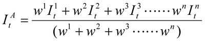
Where, superscript n represent the n^th cost item and wⁿ represents the weight assigned to the n^th cost item.

Step 3. Choice of index formula

As equation (2) shows, the aggregate price index for highway construction as a whole not only depends on the price indexes of the individual cost items of highway construction, but also depends on the weights assigned to the individual price indexes. Therefore, how to weight the individual price indexes is essential in calculating an aggregate price index, such as the NHCCI. The choice of weights also leads to the choice of index formula.

In the economic index literature, there are three well known index formulas. They are the Laspeyres Index, the Paasche Index and the Fisher Ideal Index. In equation form, they are:

(3) 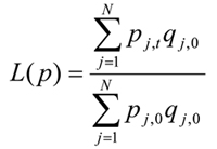(Laspeyres price index)

(4) 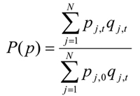(Paasche price index)

(5) 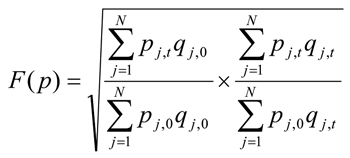(Fisher price index)

All three price index formulas use quantities of individual cost items as weights to their respective prices in calculating the aggregate price index. However, the Laspeyres price index formula uses quantities of the base period (0) as weights, while the Paasche price index formula uses quantities of the current period (t) as weights. The Fisher price index is a geometric mean of the Laspeyres price index and the Paasche price index.

Despite its many obvious advantages, the Laspeyres price index has its limitations. One of the limitations is that it usually overstates the impact of price increases and understates the impact of price decreases as the current period moves further away from the base period. This occurs because of the substitution effect when prices change in relative terms. Agents substitute away from goods whose relative prices increase so that the base year weights overstate the relative importance of these goods in the budget. As a result, the use of quantities from an earlier period as weights systematically biases the aggregate price index upward from the real change in aggregate price. In contrast, an aggregate price index derived from the Paasche price index formula is usually biased downward due to the substitution effect.

A second limitation of the Laspeyres index as it is often implemented is that as time goes on the fixed base year become less relevant to the current year or the year(s) of concern. However, if the base year is shifted forward in time, the entire index series will be changed. In other words, history will be rewritten every time the base year is changed.

The Fisher Ideal index, proposed by Irving Fisher in 1922, is one of the superlative indexes that give good approximations to the theoretical or "exact" cost-of-living index and yet are relatively simple to compute and use. Compared to fixed-weighted Laspeyres or Paasche Indexes, Fisher Ideal index takes the weights of both the base period and the current period into account. By doing so, Fisher Ideal index has the ability to accommodate the effects of substitutions, something the Laspeyres and Paasche indexes do not do. A major advantage of Fisher Ideal index over other superlative indexes, such as the Tornquvist index, is its "dual" property, i.e. a Fisher Ideal price index implies a Fisher Ideal quantity index, and vice versa. In other words, the product of a Fisher Ideal price index between two periods and a Fisher Ideal quantity index between the same two periods is equal to the total change in value (measured in current dollars) between those two periods.

All these advantages strongly suggest that the Fisher Ideal index formula is an excellent choice for building the NHCCI.

Step 4. Calculating aggregate price index for two adjacent periods

Since the OSI Bid-Tabs database provides data on bid value and bid quantity and estimated bid price data for each cost item of highway constructions in the United States, we can apply the Fisher Ideal Index formula to the bid quantity and estimated bid price data from Bid-Tabs data at the cost item (or Pay Item) level to calculate the NHCCI.

However, each time when the Fisher Ideal Index formula is applied to the price and quantity data, one and only one index number will be generated for the two time periods the data represent. In other words, the formula will not generate a price index series at once. The time period can be a month, a quarter, or a year and is usually determined by the data availability. An index number can be generated between any two periods in time. The two periods can be adjacent to each other. They also can be far away from each other with many periods between them. However, in order to build an index that accurately track price changes from one period to the next over time, it will be necessary to generate an index number for every pair of adjacent periods of the entire time period for which an index is build.

Step 5. Chain index numbers of adjacent periods into a time series of indexes

Let

:

:

:

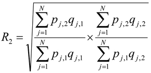
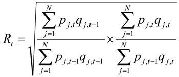
From the equations, we can see that the R₁ is the index number of period (1) relative to period (0); R₂ is the index number of period (2) relative to period (1); and R_t is the index number of period (t) relative to period (t-1); and that each index number presents the aggregate price of the current period in relative term to the aggregate price of the previous period. Mathematicians call this kind of indexing relative indexing. In relative indexing, an index number highlights the change in price from the adjacent previous period.

However, to show price changes over time, it will be more effective to compare the price of each period to the price of the base period. When an index is calculated by comparing the concerned period directly to the base period, it is called "direct indexing". The procedure of direct indexing is a dual process. That is, while the price of the concerned period is indexed in terms relative to the price of the base period, the price of the base period is also indexed to 1 and only 1. Therefore, the value of a direct index is always in terms relative to 1 and equal to the change between the two periods. This property provides the mathematical underpinning for the "chain" index procedure.

When the price of the base period (0) is indexed to 1, the chained index numbers, I₁ for period (1), I₂ for period (2), …, and I_t for period (t), can be calculated as:

(9)

:

In words, the chained index number of any period (to the base period) can be calculated as the product of the consecutive multiplication of the changes of the adjacent periods between the base period and that period. For example, with the chain-type procedure and annual rates of changes (R_t), the index of year 1995 to year 1990 (I_90,95) can be calculated as:

Summary

In summary, the Chained Fisher Ideal Index method for building the NHCCI contains two steps. In the first step, Fisher Ideal Index formula is used to calculate changes in aggregate price between adjacent periods with bid quantity and estimated bid price data at the cost item (or Pay Item) level from Oman Bid-Tabs database as inputs. This step is also an aggregation process. Changes in aggregate price of highway construction as a whole calculated in this way are essentially the averages of quantity weighted changes in the prices of the cost items of highway construction. In the second step, changes in aggregate price between adjacent periods are chained together through consecutive multiplication to form a time series of aggregate price index for highway construction as a whole.

The Chained Fisher Ideal Index method recognizes the need for estimating changes in the aggregate price of highway construction as a whole to use weights that are relevant and appropriate for the specific periods being measured. The Chained Fisher Ideal Index method has three important advantages over Fixed-Weighted Indexes. First, while it makes aggregation of price changes in many and different cost items into one measure through weighting, it captures the effects of changes in the relative importance of different cost items in highway construction over time. Second, it minimizes substitution bias and, at the same time, provides a more accurate track of price changes in highway construction cost items as a whole. Third, it eliminates the inconvenience and confusion associated with Fixed-Weighted Indexes of updating the weights and base periods, and thus rewriting economic history, as base periods move further and further into the past and become more and more irrelevant to the current.