U.S. Department of Transportation
Federal Highway Administration
1200 New Jersey Avenue, SE
Washington, DC 20590
202-366-4000
This is the first edition of the Traffic Monitoring Guide to include information on monitoring pedestrians, bicyclists, and other non-motorized road and trail users. Even though both of these modes preceded the automobile, the monitoring of non-motorized traffic has not been systematic or widespread in the U.S. and, even today, is not nearly as comprehensive as motorized traffic monitoring.
This chapter provides basic guidance intended to improve the state-of-the-practice in non-motorized traffic volume monitoring (other attributes like origin-destination, gender, and helmet use are not addressed in this Guide). In many cases, however, this guidance is limited because the systematic monitoring of pedestrians and bicyclists is still an emerging area that requires more research. Limited information is known about the best and most cost-effective ways to automatically collect non-motorized traffic data, especially because non-motorized traffic levels are typically much lower and more variable than motorized traffic levels.
One of the key differences in state-of-the-practice between non-motorized and motorized traffic monitoring is the scale of data collection. Most non-motorized data collection programs have a much smaller number of monitoring locations, and these limited location samples may not accurately represent the entire geographic area of interest. In many cases, the non-motorized monitoring locations have been chosen based on highest usage levels or strategic areas of facility improvement. Given limited data collection resources and specific data uses, these site selection criteria may be appropriate. However, one should recognize that these limited location samples might represent a biased estimate of overall usage and trends for a city or State. More research is needed to identify statistically representative site selection criteria.
A second key difference is that non-motorized traffic will typically have higher use on lower functional class roads and streets as well as shared use paths and pedestrian facilities, simply because of the more pleasant environment of lower speeds and volumes of motorized traffic. Conversely, motorized traffic monitoring focuses on higher functional class roads that provide the quickest and most direct route for motorized traffic.
A third key difference in current practice is a tendency to use very short duration counts (i.e., as short as 2 hours) for non-motorized traffic monitoring, primarily because of the perceived difficulty of automatically counting pedestrians and bicyclists (as well as the desire to collect gender and bicycle helmet use). Although this practice is not prohibited by the Guide, data users should recognize that these very short-duration counts can introduce significant overall error when non-motorized traffic use is low and inherently variable. If short-duration non-motorized counts are to be used, then it is essential that longer counts be taken to establish hourly patterns and a statistical basis for extrapolation of these counts. This issue will be addressed in more detail in Sections 4.4 and 4.5.
Finally, a fourth key difference is that technologies for counting pedestrians and bicyclists still are evolving and error rates associated with different technologies are not well known. All methods for counting both motorized and non-motorized traffic have error rates and provide estimates that only approximate actual use; however, the error rates for technologies used to count motorized traffic generally are better understood, as are the procedures for managing or reducing these errors.
This section describes the various technologies that are commonly used to count non-motorized (i.e., bicyclists and pedestrians) traffic volumes at fixed locations. The discussion differentiates between those technologies best suited to count bicyclists versus those best suited to count pedestrians. The discussion also identifies those technologies that are ideal for short-duration (i.e., portable) count locations and those that are ideal for continuous (i.e., permanent) count locations. This document does not address technologies that collect other attributes of non-motorized travel, such as the use of GPS-enabled mobile devices for trip traces or the use of Bluetooth-enabled devices for origin-destination or travel time.
Many of the basic technologies used to count bicyclists and pedestrians are similar to those used to count cars and trucks; however, the design/configuration of the sensors and the signal processing algorithms are often quite different. Therefore, separate equipment typically is used to monitor non-motorized traffic
Technological challenges to non-motorized traffic monitoring are as follows:
Selecting the most appropriate bicyclist and/or pedestrian counter can be a daunting task. Commercially available counters use a variety of technologies and features that can vary dramatically and affect how, what, where, and how long counts are collected. Cost per data point can also vary greatly between counters
Figure 4 1 presents a simplified flowchart that can help to narrow possible choices based on the two most important aspects of data collection:
1. What are you counting? Bicyclists only, pedestrians only, pedestrians and bicyclists combined, or pedestrians and bicyclists separately?
2. How long (are you counting)? Permanent, temporary, or somewhere in-between
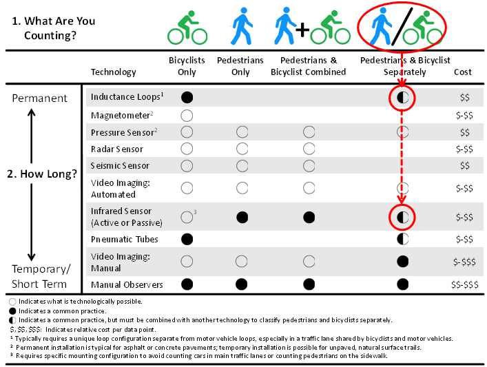
Consider the following example: a city wishes to monitor a shared-use path and would like to count bicyclists and pedestrians separately on a permanent basis. Using the simplified flowchart (Figure 4-2 for this example), the first decision point is “What are you counting?” In this example, the city wants to count both modes separately (note the circled blue and green icons in Figure 4-2). The next question in the decision process is “How long (will the counters be collecting data)?” In this example, the city wants continuous data from a permanent location, so technologies toward the middle and top of the table are relevant. Several equipment technologies are possible (e.g., pressure sensor and automated video imaging), but only a few have been used in common practice. Manual observers and video imaging with manual reduction are possible, but are typically used for short-term data collection.
For a permanent site capable of counting pedestrians and bicyclists separately, two technologies will have to be paired together. Because inductance loops are more commonly used at permanent sites, the city staff selects a combined system that has an infrared pedestrian counter paired with an inductance loop detector for bicyclists. The infrared sensor by itself is not capable of differentiating between people walking or bicycling; however, when combined with the inductance loop detector, the bicyclist counts are automatically subtracted from the infrared sensor counts.
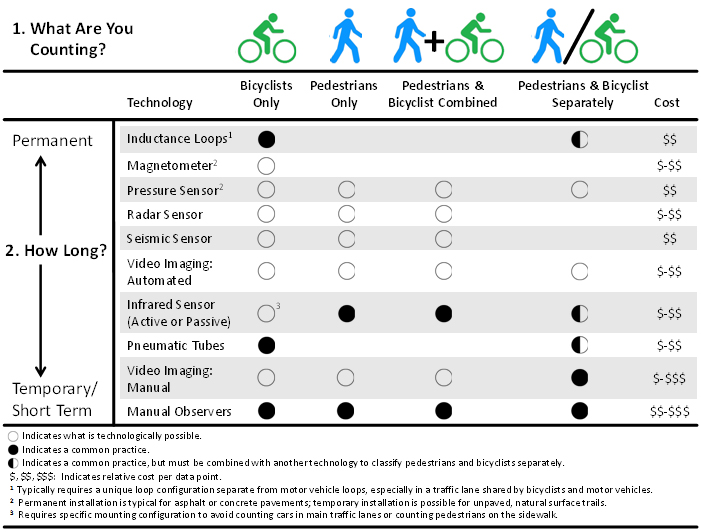
Based on budget and commercial availability, a final decision can be more easily made about technology to be deployed. Table 4-1 provides additional technology information for counting bicyclists and pedestrians, various attributes of each technology, and their strengths and weaknesses. More detailed guidance on selecting equipment for non-motorized traffic data collection is provided later in this chapter. Table 4-1 is best used after the relevant technologies have been narrowed down using Figure 4 1.
The accuracy of commercially available products can vary significantly (Turner, et al., 2007; Grembek and Schneider, 2012; Greene-Roesel et al., 2008) based on configuration, installation, and level of use, even within a specific technology (such as inductance loops for bicycles). Calibration/validation procedures (even if conducted on a limited scale) should be used to ensure that count data is within the bounds of acceptable accuracy. In fact, some local agencies have developed an equipment adjustment factor that adjusts for systematic error (e.g., undercounting) that may occur with some technologies.
| Technology | Typical Applications | Strengths | Weaknesses |
|---|---|---|---|
| Inductance Loop | Permanent counts Bicyclists only | Accurate when properly installed and configured Uses traditional motor vehicle counting technology | Capable of counting bicyclists only Requires saw cuts in existing pavement or pre-formed loops in new pavement construction May have higher error with groups |
| Magnetometer | Permanent counts Bicyclists only | May be possible to use existing motor vehicle sensors | Commercially-available, off-the-shelf products for counting bicyclists are limited May have higher error with groups |
| Pressure sensor/pressure mats | Permanent counts Typically unpaved trails or paths | Some equipment may be able to distinguish bicyclists and pedestrians | Expensive/disruptive for installation under asphalt or concrete pavement |
| Seismic sensor | Short-term counts on unpaved trails | Equipment is hidden from view | Commercially-available, off-the-shelf products for counting are limited |
| Radar sensor | Short-term or permanent counts Bicyclists and pedestrians combined | Capable of counting bicyclists in dedicated bike lanes or bikeways | Commercially-available, off-the-shelf products for counting are limited |
| Video Imaging – Automated | Short-term or permanent counts Bicyclists and pedestrians separately | Potential accuracy in dense, high-traffic areas | Typically more expensive for exclusive installations Algorithm development still maturing |
| Infrared – Active | Short-term or permanent counts Bicyclists and pedestrians combined | Relatively portable Low profile, unobtrusive appearance | Cannot distinguish between bicyclists and pedestrians unless combined with another bicycle detection technology Very difficult to use for bike lanes and shared lanes May have higher error with groups |
| Infrared – Passive | Short-term or permanent counts Bicyclists and pedestrians combined | Very portable with easy setup Low profile, unobtrusive appearance | Cannot distinguish between bicyclists and pedestrians unless combined with another bicycle detector Difficult to use for bike lanes and shared lanes, requires careful site selection and configuration May have higher error when ambient air temperature approaches body temperature range May have higher error with groups Direct sunlight on sensor may create false counts |
| Pneumatic Tube | Short-term counts Bicyclists only | Relatively portable, low-cost May be possible to use existing motor vehicle counting technology and equipment | Capable of counting bicyclists only Tubes may pose hazard to trail users Greater risk of vandalism |
| Video Imaging – Manual Reduction | Short-term counts Bicyclists and pedestrians separately | Can be lower cost when existing video cameras are already installed | Limited to short-term use Manual video reduction is labor-intensive |
| Manual Observer | Short-term counts Bicyclists and pedestrians separately | Very portable Can be used for automated equipment validation | Expensive and possibly inaccurate for longer duration counts |
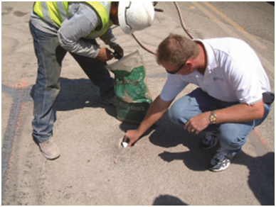
Inductance loop detectors operate by circulating a low alternating electrical current through a formed wire coil embedded in the pavement. The alternating current creates an electromagnetic field above the formed wire coil, and a conductive object (e.g., car, truck, and bike) passing through the electromagnetic field will disrupt the field by a measurable amount. If this disruption meets predetermined criteria, then detection occurs and an object is counted by a data logger or computer controller.
Inductance loop detectors do not require the presence of ferrous (i.e., iron, steel) bicycle frames; however, large conductive objects (like a car or truck) are more likely to meet the predetermined disruption criteria than smaller conductive or non-ferrous objects (like a motorcycle or bicycle). The sensitivity of an inductance loop can be changed to better detect motorcycles or bicycles, but the increased sensitivity often results in over counting for cars and trucks. For this reason, most agencies typically use dedicated loop detectors for counting bicycles rather than trying to use existing loop detectors to count cars, trucks, and bicycles.
Loop detectors are commonly used to detect the presence of motorized vehicles at or near intersections for the purposes of traffic signal control. In some cases, these loop detectors may detect the presence of bicycles. However, the location and configuration of these intersection-based loop detectors are often not ideal (and therefore rarely used) for counting purposes, both for motor vehicles and bicycles.
The preferred counting location is at mid-block or other locations where bicycles are free-flowing and/or not likely to stop. Ideally, loop detectors for bicycle counting are placed in lane positions primarily used by bicycles. If the loop detectors are placed in lanes shared by motorized traffic and bicycles, special algorithms will be necessary to distinguish the bicycles from the motorized traffic.
Inductance loop detectors are capable of measuring the direction of bicyclist travel using at least two possible options:
1. Installing an inductance loop within each directional travel lane and assuming that all (or a certain percentage) bicyclists in that lane are traveling in the specified direction (e.g., shared use path or directional bike lane).
2. Installing two inductance loops in series, such that direction can be inferred from the timing of detection events for each loop.
The first option is the most commonly used practice to date. For the second option, some data loggers or controller equipment may not be capable of interpreting signals from a paired inductance loop sequence.
The most important variables in accurate bicycle detection via a loop detector are:
QUADRUPOLE SHAPE
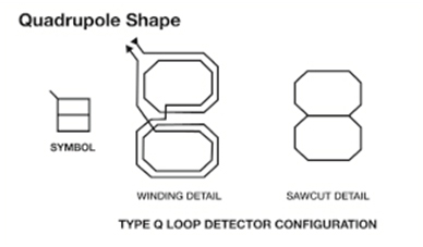
Source: Caltrans Standard Plan ES-5B, 2002.
DIAGONAL QUADRUPOLE SHAPE
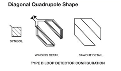
Source: Caltrans Standard Plan ES-5B, 2002.
DOUBLE CHEVRON SHAPE
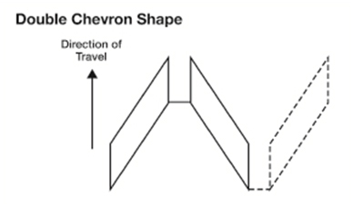
Source: Traffic Detector Handbook, 2006.
DOUBLE CHEVRON SHAPE: PHOTO
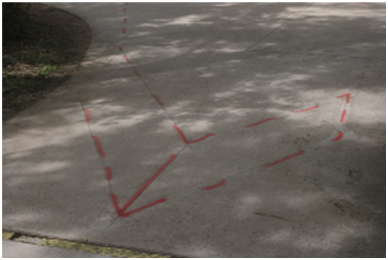
Source: Shawn Turner, TTI.
ALTERNATIVE DOUBLE CHEVRON SHAPE
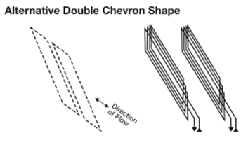
Source: Jeff Bunker, City of Boulder.
ALTERNATIVE DOUBLE CHEVRON SHAPE: PHOTO
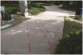
Source: Shawn Turner, TTI.
ELONGATED DIAMOND SHAPE

Source: Dan Dawson, Marin County NTPP Specifications Sheet, 2009.
ELONGATED DIAMOND SHAPE: PHOTO
Source: Shawn Turner, TTI.
Two types of infrared sensors can be easily distinguished:
Active infrared sensors have a narrower cone/zone of detection than passive infrared sensors. However, installation of active infrared sensors can be more challenging than passive infrared sensors. The transmitter and receiver parts of an active infrared sensor need to be aligned properly, and require a vertical mounting location on both sides of the detection area with a clear line of sight between. A passive infrared sensor only requires a single vertical mounting location on one side of the detection area. However, accuracy is improved when the passive infrared sensor is pointed toward a wall, building face, dense vegetation, or similar background.
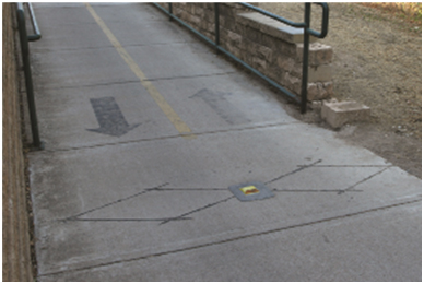
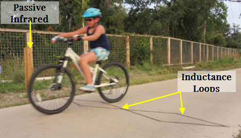
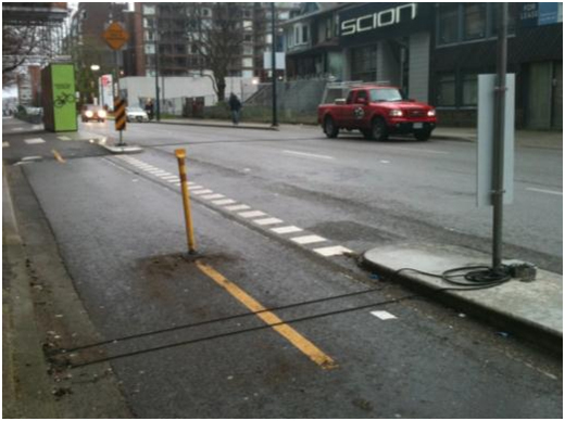
Most infrared sensors perform best in areas where the travel area is constrained and/or the detection area is well defined. Because of the basic operating principle, infrared sensors sometimes cannot distinguish multiple persons in a group (i.e., side-by-side or closely spaced front-to-back). In addition, infrared sensors cannot differentiate between bicyclists and pedestrians; therefore, if separate counts are required, infrared sensors will need to be paired with another technology able to accurately count bicycles. For example, Figure 4-4 shows a permanent monitoring location that combines a passive infrared sensor with inductance loop detectors.
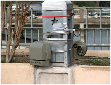
Most infrared sensors have a small profile and form factor (see Figure 4-5 for examples). For portable applications, infrared sensors can be enclosed in a vandal-resistant, lockable box and attached to an existing pole, fence post, or tree. For permanent applications, infrared sensors are often enclosed within wooden fence or other vertical posts.
Because passive infrared sensors look for heat differentials and their patterns, there may be higher error rates when the ambient air temperature approaches normal body temperature (97°-100° Fahrenheit). However, no conclusive evidence of this increased error exists, and the error may vary among different brands of passive infrared counters.
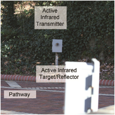
Figure 4-6 shows a typical configuration for an active infrared sensor. This example shows an ideal location: 1) primarily used by pedestrians and bicyclists only; 2) the travel area is constrained with the detector pointing across the sidewalk away from the street; and 3) the detection area is well defined in a position where pedestrians and bicyclists will be traveling perpendicular to the sensor.
Source: Shawn Turner, TTI.
Source: Shawn Turner, TTI.
Note: Equipment shown in a temporary testing and evaluation configuration
Source: Shawn Turner, TTI.
Magnetometers operate by detecting a change in the normal magnetic field of the Earth caused by a ferrous metal object (e.g., bicycle frame or components). It may be possible to use existing motorized traffic magnetometers for counting bicyclists; however, the installation and configuration may not be optimal for accurate bicyclist counting. According to the Third Edition (October 2006) of the Traffic Detector Handbook, “Magnetometers are sensitive enough to detect bicycles passing across a four-foot span when the electronics unit is connected to two sensor probes buried six inches deep and spaced three feet apart.” The shallow placement of magnetometers will result in more accurate bicyclist counts but could over count motor vehicles, as the detector might distinguish between changes in sections of the vehicle (e.g., engine block, axles, transmission) as multiple vehicles.
Magnetometers designed for motorized traffic (see Figure 4-7) may be capable of detecting bicycle frames made of non-ferrous materials (e.g., aluminum, carbon fiber, titanium), but they are not designed or optimized for this purpose. Few commercially available magnetometers designed for bicycle detection and counting exist.
Another drawback to the use of existing magnetometers for the detection of bicycles is increased equipment needs. For example, a thirty-foot detection area for automobiles would require five magnetometers and one electronic data logger. The same thirty-foot detection area would require ten magnetometers and four to five data loggers to detect bicycles.
Source: FHWA-HRT-08-001, https://www.fhwa.dot.gov/publications/publicroads/07nov/04.cfm.
Pneumatic tubes are a low-cost, portable approach for counting bicyclists only (Figure 4-8). Pneumatic tubes operate by using an air switch to detect short burst(s) of air from a passing motorized or non-motorized vehicle. The data logger then uses pre-defined criteria (e.g., axle spacing, etc.) and/or algorithms to determine whether a valid vehicle type has passed over the tubes. The technology has been used to count cars and trucks for several decades, so most public agencies either have the equipment or are familiar with the technology. Pneumatic tubes have been combined with infrared sensors at locations where both bicyclist and pedestrian counts are desired.
As with other traditional motorized traffic monitoring technology, the optimal placement and configuration of pneumatic tubes for counting bicyclists will be different from that for cars and trucks. Ideally, the placement of pneumatic tubes for bicycles should adequately cover the bicycle travel path while not being exposed to excessive passage by motor vehicles. When counting bicycles in a bike lane or shared lane, passage and activation by motorized traffic may be unavoidable. In these cases, the data logger criteria should be capable of ignoring typical motor vehicle axle spacing. If direction of bicyclist travel is desired, a pair of pneumatic tubes can be placed (see Figure 4−8), and travel direction can be inferred from the timing of detection events at each tube.
Source: Jean-Francois Rheault, Eco-Counter.
Bicyclist safety may be a concern when pneumatic tubes are installed with pavement nails or other metal fixtures, as they could possibly dislodge from the pavement and puncture a bicycle tire or create a road hazard for bicyclists. Extra care should be taken in installing pneumatic tubes, either by placing metal fixtures outside the bicycle facility or by using tape or other adhesive.
Pressure sensors operate by detecting changes in force (i.e., weight), much like an electronic bathroom scale. Seismic sensors (also sometimes called acoustic sensors) operate by detecting the passage of energy waves through the ground caused by feet, bicycle tires, or other non-motorized wheels. As with other monitoring technologies, pre-defined criteria are used to determine a valid detection and therefore a valid user to be counted.
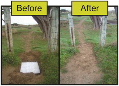
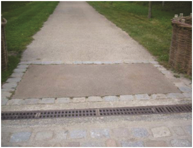
Both pressure and seismic sensors require the sensor element to be placed underneath or very near the detection area. Pressure and seismic sensors are most common on unpaved trails or paths (Figure 4-9), where burial of the sensor element is typically low-cost and minimally disruptive. However, pressure sensors have been used (more commonly in Western Europe) at curbside pedestrian signal waiting areas, as a supplement to or replacement of a pedestrian crosswalk push button
Some models of pressure and seismic sensors are capable of detecting the difference between pedestrians and bicyclists. Placement and size of the pressure sensors (also known as pressure mats) can be used to gather directional information. When installed properly, pressure and seismic sensors can serve as permanent continuous counters.
(a) Pressure sensor on natural surface trail
(b) Pressure sensor on paved surface
Source: Jean-Francois Rheault, Eco-Counter.
Video image processing operates by using sophisticated visual pattern recognition to identify (and sometimes track) a pedestrian or bicyclist traveling through a video camera’s field-of-view (see Figure 4-10). The critical element for accurate bicyclist and pedestrian counting is the pattern recognition algorithms and software. Because of the commercial demand for detecting and counting motorized traffic, this software has been extensively refined by manufacturers and vendors. Some research and development for bicyclist and pedestrian-specific algorithms has been conducted at the university level; however, much of this university research has not been incorporated into existing commercially available products.
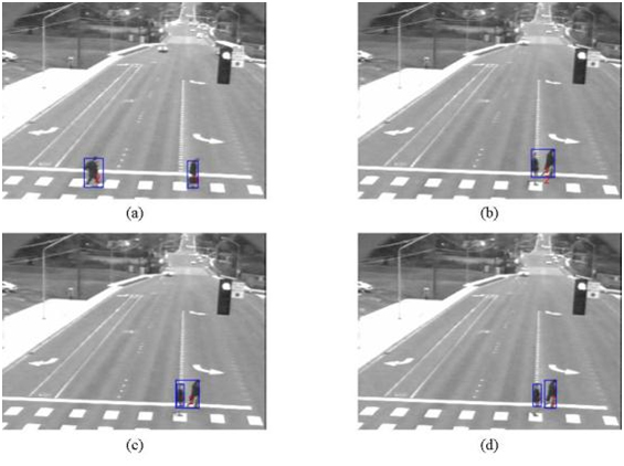
Source: Malinovskiy, Zheng, and Wang, 2009.
Video image processing has the capability to distinguish pedestrians and/or bicyclists traveling in a group or cluster. The technology also has the capability to distinguish direction of travel and potentially track the non-motorized traffic through the field-of-view. Again, these capabilities are dependent on the level of algorithm development of the commercial products. Weather and lighting may reduce the accuracy of this technology. Finally, video image processing typically has the highest equipment costs.
In some cities, pedestrian and bicyclist counts are manually reduced by viewing recorded video from intersection control or surveillance cameras. This manual approach is practical and low-cost for periodic short-term counts, but is not sustainable for continuous monitoring purposes (due to required labor and associated costs). This approach eliminates equipment installation (and corresponding traffic control), but also requires a low-cost labor force to manually review the video. Several companies offer a portable video recording unit as well as data reduction services. This recorded video may be useful to other agencies or departments that wish to study bicyclist and pedestrian behavior (e.g., in response to safety issues or concerns). Additionally, this recorded video can also be used for quality assurance purposes (i.e., for verification/validation of nearby automated counts).
The commercial marketplace for non-motorized traffic monitoring is still maturing, and several companies are still working to adapt their motorized traffic monitoring technology to accurately count bicyclists and pedestrians. For example, several companies are working to adapt their existing video image processing products to accurately count bicyclists and pedestrians. However, several companies have been successfully selling their non-motorized traffic monitoring equipment for more than a decade. An increased demand for non-motorized traffic monitoring data will provide incentives to existing companies that want to develop non-motorized traffic monitoring products.
Mobile devices with GPS and/or Bluetooth capabilities also provide a means to monitor small samples of bicyclist and pedestrian traffic. Several cities are evaluating or using these technologies to gather route choice, origin-destination, and travel time data (e.g., San Francisco, Austin, and Monterey). However, these technologies alone cannot directly count the total volumes of bicyclists and pedestrians.
Comprehensive information on non-motorized traffic variability is limited, primarily because very few public agencies have collected and analyzed continuous non-motorized traffic data to date. Future analyses will contribute a much better understanding to the traffic monitoring guidance contained here. For this section, a single continuous monitoring location (i.e., Cherry Creek Trail, Denver, Colorado) is used to illustrate variability at that site. This single example may not be indicative of non-motorized traffic variability at other U.S. locations, especially those with a mild climate year-round.
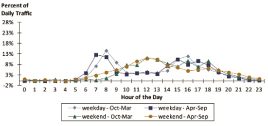
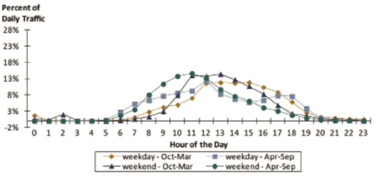
The time-of-day variation for mixed-mode (i.e., pedestrians and bicyclists), non-motorized traffic at a single location is shown in Figure 4-11. The time-of-day patterns for non-motorized traffic data will vary by location and trip purposes. The time-of-day patterns are somewhat different from car and truck patterns (Figure 1-2), but similarities do exist. Diurnal peaking patterns can be seen during the weekdays for non-motorized traffic; however, the non-motorized peaks are less pronounced than the car and truck peaks. The weekend profiles for non-motorized traffic have a single peak (same as rural cars), but the non-motorized peak is mid-day (as opposed to an evening peak for rural cars) and is much more pronounced (12%-13% for non-motorized as compared to 8% for rural cars). For this trail in Colorado, the time-of-day patterns for non-motorized traffic do vary by season of the year.
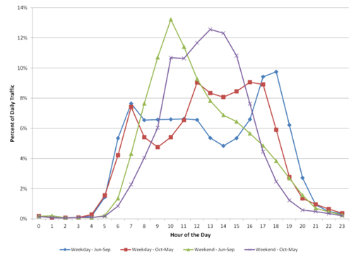
Source: Cherry Creek Trail continuous count data, Colorado Department of Transportation, 2010.
Figure 4-12 shows average hourly traffic profiles from 12-hour manual counts of bicyclists and pedestrians on 43 weekdays in Minneapolis, Minnesota. This data illustrates one of the limitations of manual counting relative to automated counting: it is expensive and difficult to obtain 24 hour counts. However, these counts illustrate patterns in time-of-day use and that peak hour counts correlate well with 12-hour counts. This data also underscores the importance of longer-duration counts so that the limitations of short duration (e.g., two hour) counts can be understood and interpreted.
Figure 4-12 also illustrates that different time-of-day traffic patterns may occur when pedestrian and bicyclist modes are reported separately. In this case, pedestrian traffic has a much stronger mid-day peak than bicyclists. If automated counter equipment can differentiate pedestrians from bicyclists, then counts should be stored separately by mode to permit analysis and reporting by mode (if desired).
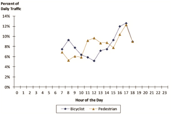
Source: Greg Lindsey, University of Minnesota.
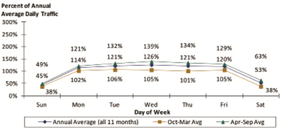
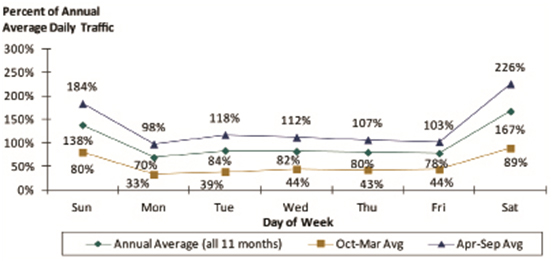
The DOW variation for mixed-mode non-motorized traffic at a single location is shown in Figure 4-13. The overall profile of the non-motorized traffic is similar to the recreational car or through truck as shown in Figure 1-4. However, the weekend traffic is more pronounced for the non-motorized trail traffic. The other significant difference is how the magnitude varies by season of the year. As shown in Figure 4 13, the typical DOW traffic during the summer and early fall months (June through September) are nearly twice that during the winter and spring months (October through May).
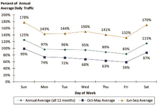
Source: Cherry Creek Trail continuous count data, Colorado Department of Transportation, 2010.
The DOW patterns shown in Figure 4 13 are averaged over a full year. The actual day-to-day variation of non-motorized traffic volumes will be substantially greater than shown in this figure. Adverse weather (e.g., heavy rain, extreme hot or cold temperatures) has a significant impact on bicycling and walking traffic levels. In fact, even forecasts of adverse weather may also have an impact on non-motorized traffic.
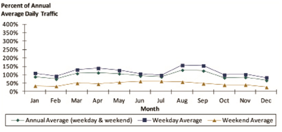
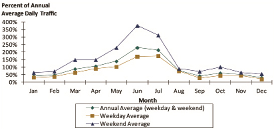
The monthly variation for mixed-mode, non-motorized traffic at a single location in Colorado is shown in Figure 4 14. The overall monthly patterns are similar to the rural car and truck patterns in Figure 1-5; however, the seasonality for non-motorized traffic is much more pronounced. For example, the peak summer non-motorized traffic during July is about 200%, or nearly twice the annual average. The winter non-motorized traffic (November through February) is about 50%, or one-half of the annual average. Figure 4-14 clearly demonstrates the seasonal effects on non-motorized traffic at this Colorado location
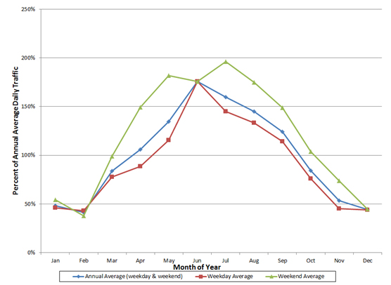
Source: Cherry Creek Trail continuous count data, Colorado Department of Transportation, 2010.
Figure 4-15 illustrates similar monthly patterns at six shared use path locations in Minneapolis, Minnesota where weather is more seasonal, with colder winters and more humid summers. The Minneapolis data, which are quite similar across the six locations, show greater seasonality than the Colorado data, with average daily traffic in summers more than double the annual average daily traffic, and winter (e.g., January) daily traffic well below 25% of annual average daily traffic. These two examples illustrate the importance of understanding the effects of weather and seasonality on non-motorized traffic
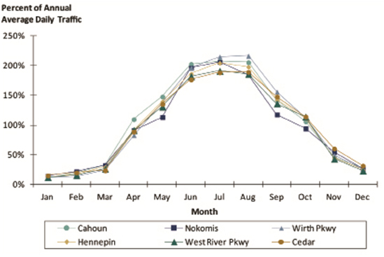
Source: Greg Lindsey, University of Minnesota.
The variability described in the previous sections should be measured and accounted for in a non-motorized traffic data collection and reporting program. The data collection program should also identify changes in these traffic patterns as they occur over time. To meet these needs in a cost effective manner, statewide traffic monitoring programs generally include:
The short duration counts provide the geographic coverage to understand traffic characteristics on individual roads, streets, shared use paths, and pedestrian facilities, as well as on specific segments of those facilities. They provide site-specific data on the time of day variation, can provide data on DOW variation in non-motorized travel, but are mostly intended to provide current general traffic volume information throughout the larger monitored network. However, short duration counts cannot be directly used to provide many of the required data items desired by users. Statistics such as annual average traffic cannot be accurately measured during a short duration count. Instead, data collected during short duration counts are factored or adjusted to create these annual average estimates. The procedures to develop and apply these factors are discussed in Section 4.4.
The development of those factors requires the operation of at least a modest number of permanently operating traffic monitoring sites. Permanent data collection sites provide data on seasonal and DOW trends. Continuous count summaries also provide very precise measurements of changes in travel volumes and characteristics at a limited number of locations.
The process for collecting continuous non-motorized traffic data should follow the steps already outlined for motorized traffic in Chapter 3, as follows:
1. Review the existing continuous count program;
2. Develop an inventory of available continuous count locations and equipment;
3. Determine the traffic patterns to be monitored;
4. Establish pattern/factor groups;
5. Determine the appropriate number of continuous monitoring locations;
6. Select specific count locations; and
7. Compute monthly, DOW, and hour-of-day (if applicable) factors to use in annualizing short-duration counts.
The following sections provide additional detail for implementing these steps.
In this edition of the Traffic Monitoring Guide, pedestrians and bicyclists are grouped together as non-motorized traffic. There will be differences in these two types of facility users that may affect the monitoring approach. However, the known distinctions and differences between pedestrian and bicyclist traffic will be pointed out in each combined section. As ongoing research identifies the best approach for each, future editions of the Guide may provide additional information for separate monitoring of pedestrian traffic and bicyclist traffic.
The first two steps are to inventory, review, and assess what your agency currently has (in regard to permanent monitoring locations and equipment). This may be a short exercise for some agencies, as permanent continuous counts are much less common than short-duration pedestrian and bicyclist counts.
However, these first two steps should not be bypassed simply because your own agency does not have permanent count locations. Because non-motorized traffic levels are typically higher on lower-volume and lower functional class roads/streets as well as shared use paths and pedestrian facilities, city and county agencies and metropolitan planning organizations (MPOs) have often been more active than State DOTs in monitoring non-motorized traffic
Therefore, if a State DOT traffic data collection program will monitor non-motorized traffic, they should coordinate with local and regional agencies as they inventory and review existing continuous counts. Additionally, they should inquire with departments other than the transportation or public works department. The following lists possible agencies and/or departments that may have installed permanent pedestrian and bicyclist counters:
The process outlined in Section 3.2.1 for motorized traffic volume is equally applicable for non-motorized traffic. The review of existing continuous counts should review and assess the following:
If existing continuous count data is available, it should be analyzed to determine typical traffic patterns and profiles:
Note that the count magnitude may not be similar, but the time-of-day, DOW, or month-of-year patterns may be similar in shape or overall profile. These patterns of variation will ultimately be used to create groups of similar locations (called factor groups) that can be used to factor (i.e., annualize) short-duration counts to an annual volume estimate.
If continuous non-motorized count data is not available, short-duration counts can be used to estimate the traffic patterns that may be typical. However, because of the higher variability of pedestrian and bicyclist count data, short-duration counts should be used with great caution. Short-duration counts cannot be used to determine monthly variability and, depending on the duration of the counts, may not be indicative of typical DOW variability. In addition, inclement weather or other special events may skew the time-of-day patterns in short-duration counts. In most cases, though, some data is better than no data in establishing typical traffic patterns.
In reviewing the current program and existing non-motorized data, one should also understand the basics of how data is processed by the field equipment and loaded into its final repository, whether that be a stand-alone spreadsheet, a mode-specific database, or a traffic monitoring data warehouse. The following elements should be considered:
Subjective data manipulation or editing should be avoided. Instead, appropriate business rules and objective procedures can be used in combination with supporting metadata to address missing or invalid data.
The final step in reviewing the existing program is to consider summary statistics, both those that are currently computed as well as those that may be needed. Permanent count locations should be providing count data 24 hours per day, 365 days per year; however, this continuous data stream is often summarized into a few basic summary statistics, like annual average daily traffic. Because of the greater monthly variability of non-motorized traffic, other summary statistics may be more relevant:
The review of existing and needed summary statistics should be based on those users and uses that have been identified earlier in this process. In this way, one can ensure that the variety of users has the required information to make decisions.
After reviewing the existing non-motorized program (both what is being done and what is needed), Step 3 is to determine those traffic patterns that are to be monitored. Part of this determination will depend upon the functional road classes and bicyclist and pedestrian facilities of interest. For example, do State DOTs want to collect pedestrian and bicyclist count data on local streets, shared use paths, and pedestrian facilities that are considered off-system (i.e., not included on the State highway system)? In some cases, State DOT funding has been used for non-motorized projects on local streets and shared use paths through the Transportation Enhancements (TE) or Congestion Mitigation and Air Quality (CMAQ) funding categories.
Once the non-motorized network to be monitored has been defined, one should determine the most likely types of traffic patterns that are expected on this network. In most cases, the non-motorized network will include facilities that have a mix of commute, recreational, and utilitarian trips. Depending upon the relative proportions of these different trip types, distinct traffic patterns will emerge. These patterns should be used in the Step 4 to establish seasonal pattern groups.
The most common way to determine typical traffic pattern groups is through the visual analysis and charting of existing data. Continuous count data is preferred for this step, but short-duration counts (multiple full days, but not two-hour counts on a single day) may also be used with caution.
In the previous step (Step 3), existing non-motorized data was used to determine the traffic patterns that are to be monitored. In Step 4, this information is used to establish unique traffic pattern groups that will be used as the foundation for the monitoring program. In some cases, non-motorized count data may not be available in Step 3 to determine the most likely traffic pattern groups. In these cases, previous analyses of non-motorized data from previous studies or of similar locations should be used as a starting point. Once more non-motorized data is gathered in your region, these traffic pattern groups can be refined based on your local data.
Previous (but limited) research indicates that non-motorized traffic patterns can be classified into one of these three categories (each with their own unique time-of-day and DOW patterns):
For example, Figures 4-16, a-b-c shows typical traffic patterns for a permanent monitoring location that has a higher percentage of commuting-based trips:
HOUR OF DAY
Source: Continuous Count Data, Colorado Department of Transportation, 2010-2011.
DAY OF WEEK
Source: Continuous Count Data, Colorado Department of Transportation, 2010-2011.
MONTH
Source: Continuous Count Data, Colorado Department of Transportation, 2010-2011.
Figures 4-17, a-b-c show typical traffic patterns for a permanent monitoring location that has a higher percentage of recreation-based trips:
HOUR OF DAY
Source: Continuous Count Data, Colorado Department of Transportation, 2010-2011.
DAY OF WEEK
Source: Continuous Count Data, Colorado Department of Transportation, 2010-2011.
MONTH
Source: Continuous Count Data, Colorado Department of Transportation, 2010-2011.
Overall climate conditions will strongly influence seasonal patterns. Day-to-day weather conditions will also influence specific daily or weekly patterns, but should not have a seasonal impact.
Facility type and adjacent land use are important variables; however, these will influence the mix of trip purpose, which is likely the strongest predictor of time-of-day and DOW traffic patterns.
Very little is known about spatiotemporal variation of non-motorized traffic, and what is known is very location-specific and difficult to generalize nationwide. In most cases (where no non-motorized counting currently exists), the number of count locations will be based on what is feasible given existing traffic monitoring budgets.
If equipment budgets are not constrained, then a rule of thumb is that about three to five continuous count locations should be installed for each distinct factor group (based on trip purpose and seasonality). The number of permanent count locations can be refined and/or increased as more data is collected on non-motorized traffic.
Once the number of locations within factor groups has been established, the next step is to identify specific monitoring locations. Several considerations should be addressed in this step.
Differentiating pedestrian and bicyclist traffic – Will pedestrian and bicyclist traffic be separately monitored at each permanent count location? In the case of shared use paths, pedestrians and bicyclists will be traveling in the same space, and specialized equipment should be used to differentiate these different user types. In other situations, it may be preferable to monitor bicyclists separately from pedestrians. Exclusive bicycle lanes or separated bicycle paths can be instrumented with inductance loops (permanent) or pneumatic tubes (short-duration) that will not count larger/heavier motorized vehicles. Pedestrian malls, sidewalks or walkways can be instrumented with a single-purpose infrared counter if bicyclists are not typically present.
Selecting representative permanent count locations – Although it may be tempting to select the most heavily used locations for permanent monitoring, one should focus primarily on selecting those locations that are most representative of prevailing non-motorized traffic patterns (while still having moderate non-motorized traffic levels). In some cases, permanent count locations may be installed at low-use locations if higher use is expected after pedestrian or bicycle facility construction. The primary purpose of these continuous monitoring locations is to factor/annualize the other short-duration counts. Continuous counts at a high-pedestrian or high-bicyclist location may look impressive, but may not yield accurate results when factoring short-duration counts
Selecting optimal installation locations – Once a general site location is identified, the optimal installation location should be chosen for the specific monitoring technology and equipment. In most cases, the optimal location is:
The computation of adjustment factors should follow a similar process as motorized traffic volumes outlined in Section 3.2.1. These adjustment factors will be calculated for each unique non-motorized traffic factor group as determined in Step 4.
In practice, very few agencies have applied monthly or DOW adjustment factors to short-duration non-motorized counts. The current prevailing practice is to collect short-duration counts during those dates and times that are believed to be average, thereby reducing the perceived need for adjustment. However, this practice should evolve to a more traditional traffic monitoring approach as more permanent non-motorized count locations are installed.
Similar to motorized traffic monitoring, the majority of non-motorized locations will be monitored using short-duration counts. However, in some non-motorized monitoring programs the distinction between short-duration counts and special needs counts is not clearly defined. Short-duration counts are performed on specific facilities based on certain needs for that facility (e.g., before-after), but it is not known whether that specific facility is representative of other facilities and can therefore be expanded to a sub-area or regional estimate of overall non-motorized travel.
Unfortunately, clear guidance does not yet exist on this statistical representation issue and one will have to use their best judgment in determining which special needs counts also can be used to represent sub-area or regional travel estimates and trends.
For motorized traffic, State DOTs have a short-duration data program that provides traffic data for all roads on their State highway system. The same goal for non-motorized traffic data may not be feasible, especially since most non-motorized travel occurs off the State highway system and on lower-volume and lower-speed city streets, shared use paths, and pedestrian facilities.
The prevailing practice for collecting short-duration non-motorized traffic data has been to focus on targeted locations where activity levels and professional interest are the highest. Although this non-random site selection may not yield a statistically representative regional estimate, it provides a more efficient use of limited data collection resources (e.g., random samples could possibly result in many locations with low or very low non-motorized use).
The following National Bicycle and Pedestrian Documentation (NBPD) Project criteria are recommended for short-duration counts:
The number of short-duration count locations will depend on the available budget and the planned uses of the count data. To date, there has been no definitive analysis of, or guidance for, determining the required number of short-duration count locations. For most regions getting started with counting non-motorized travel, the short count program is best developed by working with other key stakeholders interested in collecting and using this data. By discussing needs and budgets, this group can identify and prioritize the special needs short count locations which the available data collection budget can afford to collect. (These same discussions should also identify those key regional facilities that should be used for early deployment of permanent counters that will then be used to expand the short count data into estimates of annual and peak use.) The special needs counts will then provide the data needed to guide the development of a more statistically valid sample of short count locations. These more statistically rigorous sample designs will become possible in the future as more data is collected and as research is performed in the coming years.
Once general monitoring locations have been identified, the most suitable counter positioning should be determined. The NBPD Project recommended the following guidance for counter positioning:
In many cases, these recommended counter-positioning locations will result in the highest non-motorized traffic volumes. Given limited data collection resources and specific data uses, this focus on high-use locations may be appropriate. However, one should recognize that these high-use locations might represent a biased estimate of use levels and trends for an entire city or State.
The two basic location types for non-motorized traffic monitoring are:
1.Screen line counts that are taken at a mid-segment location along a non-motorized facility (e.g., sidewalk, bike lane, cycle track, shared use path); and,
2. Intersection crossing counts that are taken where a non-motorized facility crosses another facility of interest.
Screen line counts are typically used to identify general use trends along a facility, and are analogous to most short duration motorized traffic counts. Although taken at a specific location, screen line counts are sometimes applied to the full segment length to calculate vehicle-miles of travel, pedestrian-miles of travel, and bicyclist-miles of travel.
Intersection crossing counts are typically used for safety and/or operational purposes, and are most analogous to motorized intersection turning movement counts. Example applications include using intersection counts to determine exposure rates at high collision crossings, as well as to retime or reconfigure traffic signal phasing. Intersection counts are typically more complicated than screen line counts and may require additional counters, primarily because multiple intersection approaches are being counted at once.
The uses of the non-motorized traffic data will dictate which types of counts are most appropriate.
There is no definitive guidance on the minimum required duration of short-duration counts. The prevailing practice has been two consecutive hours on a single day, but that practice is evolving as more public agencies use automatic counters and become aware of the inherent variability of non-motorized traffic. The following paragraphs discuss several factors that agencies should consider when determining the duration of their short-duration counts.
The use of automatic counter equipment can dramatically extend the duration of short-duration counts. If automatic counters are used, then the minimum suggested duration is 7 days (such that all weekday and weekend days are represented). Depending on several other factors (e.g., day-to-day count variability, the total number of short-duration monitoring sites, and the number of automatic counters), the preferred duration of automatic counts could be as long as 14 days at each location.
The use of manual observers will limit the duration of short-duration counts. However, the minimum suggested duration for manual observers is 4 to 6 hours and should be scheduled to coincide with the heaviest non-motorized use (typically mid-day for weekend/recreational trips and morning/evening commute times for other trips). Manual observers’ counting accuracy declines after 2 hours, so observers should be given short breaks or replaced with other observers. The preferred length for short-duration counts is 12 hours, which permits calculation of time-of-day use profiles. However, it is recognized that available resources may limit the collection of 12-hour counts.
The prevailing practice for short-duration manual counts has been 2 hours, largely because of resource and manual observer limitations. There is recognition that 2 hours of count data is better than no data; however, 2 hours of count data may lead to high error rates when annualizing counts and could lead to erroneous conclusions. If manual observers are the only possibility for short-duration counts, then agencies are encouraged to count for longer periods at fewer locations. Alternatively, the NBPD project (National Bicycle and Pedestrian Documentation Project: Instructions) has encouraged agencies to count multi-hour periods on several different days:
“We suggest that between 1 and 3 counts be conducted at every location on sequential days and weeks, based on the approximate levels of activity. Areas with high volumes (over 100 people per hour during midâ€�day periods) can usually be counted once on a weekday and weekend day, unless there is some unusual activity that day or land use nearby.”
“Areas with lower activity levels and/or with unusual nearby land uses (with any irregular activity, such as a ball park) or activity (such as a special event) should be counted on sequential days or weeks at least one more and possibly two more times.”
If non-motorized traffic levels are high and consistent from day-to-day, then shorter periods and/or fewer days may be considered. However, a longer-duration count period will be needed to determine how variable the non-motorized traffic is by time-of-day and DOW. Unfortunately, there is little quantitative guidance or consensus in this area, and ongoing research will improve future guidance.
Weather can be a significant factor in the level and variability of non-motorized traffic and should be considered when developing a short-duration monitoring program. Seasonal weather patterns (such as cold winters or hot/humid summers) are expected by pedestrians and bicyclists and will result in relatively consistent patterns from year to year. However, heavy precipitation or unexpectedly hot or cold weather may introduce abnormal variations on a given time of day or day of year. These variations can both generate unusually high levels of activity (e.g., a very nice day) or depress otherwise expected levels of activity (due to very bad weather.)
If automatic counter equipment is used for short-duration counts in typical weather, then the minimum suggested duration is 7 days (such that all weekday and weekend days are represented). This duration provides an average of 5 weekdays and 2 weekend days. However, if atypical heavy precipitation or inclement weather occurs during this entire 7-day period, agencies should consider extending the duration to 14 days.
When heavy precipitation or inclement weather occurs with manual observers, the counts should be extended over multiple days at the same time. Local judgment should be used to determine whether to include inclement-weather days into a multi-day average.
Because of inclement weather’s influence on non-motorized traffic, weather conditions should be recorded in a non-motorized traffic monitoring program. The non-motorized data submittal format in Chapter 7 recommends three weather-related attributes:
1. Precipitation (yes/no): Did measurable precipitation fall at some time during data collection?
2. High temperature: Approximate high temperature for either the day (if a day or longer count) or the duration of the count (if the count is less than a day in duration
3. Low temperature: Approximate low temperature for either the day (if a day or longer count) or the duration of the count (if the count is less than a day in duration
Historical weather data can be obtained from several different sources and does not necessarily have to be collected at the exact count location.
The specific months/seasons of the year for short-duration counts should be chosen to represent average or typical use levels, which can be readily determined from permanent continuous counters (thereby underscoring the importance of these automatic continuous counters). In most climates in the U.S., the spring and fall months are considered the most representative of annual average non-motorized traffic levels (e.g., the NBPD projects recommends mid-May and mid-September).
Short-duration counts may be collected during other months/seasons of the year that are not considered average or typical; however, a factoring process will be necessary to adjust these counts to best represent an annualized estimate of non-motorized traffic
As indicated in the previous section, a factoring process may be necessary to adjust short-duration counts to best represent an annualized estimate. The factoring process for motorized traffic has been described in depth in Chapter 3. It is recommended that a similar factoring process be used to annualize non-motorized traffic counts.
Depending on the count duration, type of automated equipment used, and presence of inclement weather, there may be up to five factors that could be applied:
1. Time-of-day: If less than a full day of data is collected, this factor adjusts a sub-daily count to a total daily count.
2. DOW: If data is collected on a single weekday or weekend day, this factor adjusts a single daily count to an average daily weekday count, weekend count, or day of week count.
3. Month/season-of-year: If less than a full year of data is collected, this factor adjusts an average daily count to an annual average daily count.
4. Occlusion: If certain types of automatic counter equipment are used, this factor adjusts for occlusion that occurs when pedestrian or cyclists passing the detection zone at the same time (i.e., side-by-side or passing from different directions).
5. Weather: If short-duration counts are collected during periods of inclement weather, this factor adjusts an inclement weather count to an average, typical count.
Adjustment factors are developed for distinct factor groups, which are groups of continuous counters that have similar traffic patterns. The continuous counters in the factor groups provide year-round non-motorized traffic counts and permit these short-duration counts to be annualized in a way that minimize error.
The non-motorized data submittal formats in Chapter 7 provide the capability to report these five types of adjustment factors in five separate factor groups
Although factoring is a straightforward mathematical process, very few agencies are using factor groups for non-motorized traffic counts. There is no consensus yet on several aspects of the factoring process, such as the required type of factor adjustments, the number of factor groups for each adjustment type, and the number of continuous count locations within each factor group. It is hoped that future editions of the Guide will be able to provide additional guidance on this non-motorized count factoring process.
Many State DOTs do have data warehouse tools that already perform the factoring process for motorized traffic counts. Many of these tools and factoring processes could be used for non-motorized traffic factoring, given some adaptation as discussed.
The following is a simplified example that illustrates the process of calculating an estimate of average annual traffic based on a short-duration count. The example (Lindsey, G., Chen, J., Hankey, S., and Wang, X., 2012.) uses adjustment factors from a permanent monitoring location to annualize the short-duration counts. The example is for mixed-mode non-motorized traffic (i.e., bicyclists and pedestrians combined) along the Midtown Greenway, a shared-use path in Minneapolis, Minnesota. An active infrared counter was used at the permanent monitoring location along the Greenway, near an intersection with Hennepin Avenue.
Table 4-2 presents the following actual mixed-mode traffic count statistics for 2011 at the Hennepin Avenue monitoring location along the Midtown Greenway
The steps in using these factors to obtain estimates of annual traffic and AADT for Site A are:
1. Use the 2011 Friday and Saturday mean daily traffic ratios for February to calculate an average adjustment factor for the February 2012 48 hour monitoring period.
2. Estimate the MADT for February 2012
3. Use the MADT/AADT ratio from February 2011 to estimate the 2012 AADT and 2012 annual traffic. From Table 4-2, the average Friday traffic in February 2011 was 1.04 times February average daily traffic, and the average Saturday traffic was 1.27 times February average daily traffic. Therefore, for the Friday-Saturday monitoring period, the average daily traffic was 1.16 times the February average daily traffic.
4. Using this ratio, the 2012 February average daily traffic can be calculated from the 2012 48-hour traffic count:
2012 February average daily traffic = (175 + 250) / 1.16 = 183
5. From Table 4-2, the February MADT/AADT ratio is 0.18 (i.e., February average daily traffic is 18% of annual average daily traffic). This factor then is used to calculate AADT and annual traffic for 2012 for Site A:
Site A AADT = (183 / 0.18) = 1,023
Site A cumulative annual traffic = 1,023 × 365 = 373,422
This example could easily be extended for counts of different duration (e.g., daily or weekly or peak hour). To extrapolate two-hour, peak hour counts, hourly adjustment factors from the continuous monitoring sites would be needed. While the general process would be the same, extrapolation from peak hour counts would introduce additional uncertainty into the estimates of AADT and annual traffic.
Jan |
Feb |
Mar |
Apr |
May |
Jun |
Jul |
Aug |
Sep |
Oct |
Nov |
Dec |
|
|---|---|---|---|---|---|---|---|---|---|---|---|---|
| Annual Average Daily Traffic | 1,975 |
1,975 |
1,975 |
1,975 |
1,975 |
1,975 |
1,975 |
1,975 |
1,975 |
1,975 |
1,975 |
1,975 |
| Monthly Average Daily Traffic (MADT) | 239 |
354 |
586 |
1,807 |
2,753 |
3,699 |
4,099 |
3,896 |
2,805 |
1,960 |
886 |
495 |
| Ratio of MADT to AADT | 0.12 |
0.18 |
0.30 |
0.92 |
1.39 |
1.87 |
2.08 |
1.97 |
1.42 |
0.99 |
0.45 |
0.25 |
| Ratio of Sunday ADT to MADT | 0.89 |
1.33 |
0.89 |
1.55 |
0.88 |
1.29 |
1.18 |
1.34 |
1.06 |
1.20 |
0.75 |
1.11 |
| Ratio of Monday ADT to MADT | 1.01 |
0.66 |
1.10 |
1.10 |
0.98 |
0.95 |
0.98 |
0.87 |
1.22 |
0.96 |
1.00 |
1.08 |
| Ratio of Tuesday ADT to MADT | 1.10 |
0.74 |
0.91 |
0.96 |
1.27 |
0.89 |
0.91 |
0.74 |
0.86 |
1.03 |
1.01 |
1.07 |
| Ratio of Wednesday ADT to MADT | 1.15 |
0.96 |
0.93 |
0.76 |
1.11 |
0.96 |
0.94 |
1.07 |
0.99 |
0.87 |
1.03 |
0.97 |
| Ratio of Thursday ADT to MADT | 1.06 |
1.00 |
1.03 |
0.88 |
0.93 |
0.96 |
0.90 |
1.03 |
0.85 |
0.87 |
0.97 |
0.92 |
| Ratio of Friday ADT to MADT | 0.97 |
1.04 |
0.84 |
0.78 |
0.79 |
0.96 |
0.95 |
0.88 |
0.87 |
0.82 |
1.31 |
0.91 |
| Ratio of Saturday ADT to MADT | 0.88 |
1.27 |
1.34 |
1.03 |
1.02 |
1.02 |
1.09 |
1.15 |
1.23 |
1.16 |
0.91 |
0.98 |
Source: Greg Lindsey, University of Minnesota.

