U.S. Department of Transportation
Federal Highway Administration
1200 New Jersey Avenue, SE
Washington, DC 20590
202-366-4000
This chapter describes Federal guidelines for establishing and maintaining traffic monitoring programs. Detailed guidance is provided for traffic monitoring methodologies ranging from determining the number of data collection stations, to how to assign factor groups using cluster analysis as one of the tools.
This chapter is organized into the following sections:
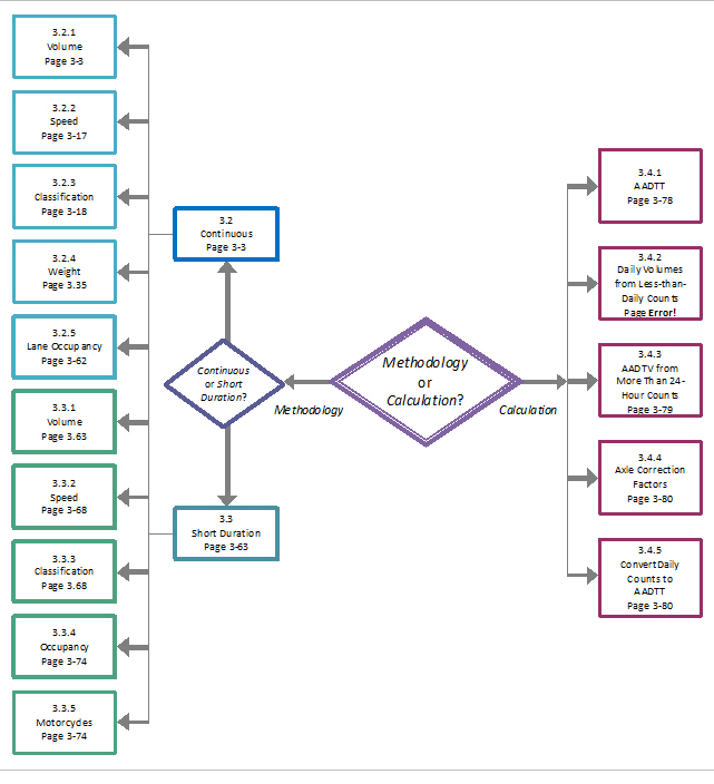
The Figure 3-1 is a chapter map showing how the sections relate to each other. Please note that some of the sections repeat certain information and guidance. This is to ensure all relevant points are made in every relevant section
Source: Federal Highway Administration
In most States, the continuous count stations form the basis for the overall traffic monitoring program. The definitions related to continuous count programs are included in Chapter 1. A continuous count is a volume count derived from permanently installed counters for a period of 24 hours each day over 365 days (except for leap year) for the data-reporting year. There is an attempt to collect 365 days of data per year, but sometimes data is not available for some of those days. In some States, this is referred to as the permanent count program. In the TMG, the program will be referred to as the continuous count program.
The objectives of continuous count programs are many and vary from State to State. Continuous count stations can be used to develop adjustment factors, track traffic volume trends on important roadway segments, and provide inputs to traffic management and traveler information systems. The number and location of the counters, type of equipment used, array, sensor technology, and the analysis procedures used to manipulate data supplied by these counters are functions of these objectives. As a result, it is of the utmost importance for each organization responsible for the implementation of the continuous count program to establish, refine, and document the objectives of the program. Only by thoroughly defining the objectives, and designing the program to meet those objectives, will it be possible to develop an effective and cost-efficient program.
Volume data is normally collected as part of a State’s continuous count program. The primary objective of the program is to develop hour of day (HOD), day of week (DOW), month of year (MOY) and yearly factors to expand short-duration counts to AADT. This objective is the basis for establishing the number and location of continuous count sites operated by the State highway agency. Secondary objectives of the continuous count program include the following:
Each agency develops its own balance between having larger numbers of continuous count stations (increasing the accuracy and reliability of analyses that depend on data supplied by those counters) and reducing the expenditures required to operate and maintain those counters. The TMG recommendations provide sufficient flexibility for each agency to find an appropriate compromise among objectives.
When determining the balance point, the objectives of the continuous count program should be statewide in nature, and the focus should reflect this statewide perspective (see Appendix D, Case Studies #1 and #2). As a result, the continuous count program should be developed to meet the minimum requirements of the State highway agency for ensuring statistical validity. Sub-area and roadway-specific data collection needs should be secondary considerations in the design of the continuous count program as desired by the appropriate agency.
Consequently, the TMG recommends that the division responsible for factor development operate at least the minimum number of continuous count locations needed to meet the accuracy and reliability requirements of the factoring program. Expansion of the data available through the program should come from other available count programs. That is, data available through other count programs such as intelligent transportation systems (ITS), MPOs, cities, counties and WIM programs (if separate), where the funding for the installation and operation of the counters comes from other sources, should be considered to supplement and expand the continuous count database (See Chapter 5, Case Studies #1 through #5). However, while the cost of equipment installation and operation of these supplemental continuous count programs is the responsibility of those other programs, the statewide traffic monitoring division should be responsible for ensuring its accuracy and making this data available to users. Determining how best to obtain, summarize, and report this data is an issue best addressed at the State level. Data management best practices can be learned from advanced travel monitoring programs. These examples are provided in Appendices D, E, and L.
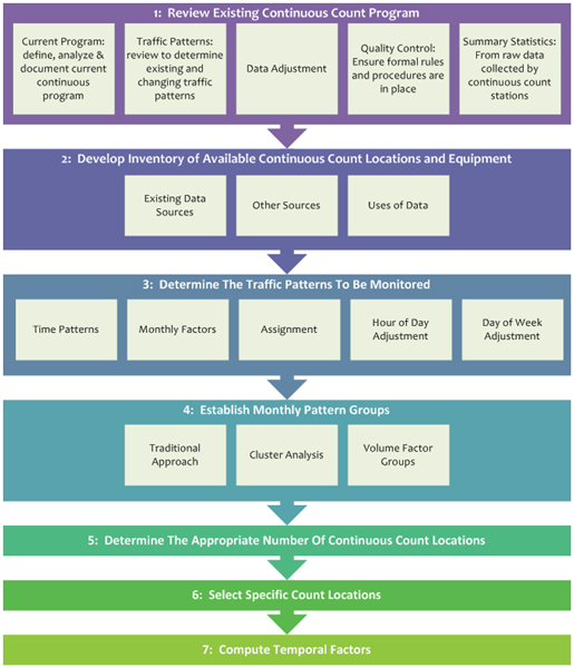
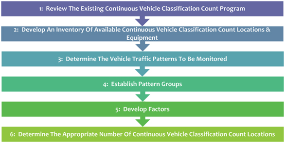
Several steps should be followed in establishing and evaluating a continuous count program for statewide traffic monitoring. The results of those steps will allow for benchmarking and improving the monitoring program. The lists were designed for 1) developing a new program; 2) checking to ensure compatibility with the guidance; and 3) evaluating a program.
The following figure shows the steps to be followed in establishing a volume program.
VOLUMES
Source: Federal Highway Administration
A. Current Program – The first step in refining the continuous count system is to define, analyze, and document the current continuous count program. A clear understanding of the current program will increase confidence in later decisions to modify the program. The review should explore the historical design, procedures, equipment, personnel, objectives, and uses of the information. This review should start with an inventory of the continuously operating traffic data collection equipment available (this would include features, limitations, age, and repair/failure rates). It should then progress to determining how the data is being used, who is using it, and how it would be used if tools for using it in new ways were available
B. Traffic Patterns – Next, the data should be reviewed to determine hourly, daily, and monthly traffic patterns that exist in the State and whether previous patterns have changed in order to establish whether the monitoring process should also change.
C. Data Adjustment – The next step is to review how the data is being adjusted, and whether those data adjustment steps can be improved or otherwise made more efficient. Of considerable interest in this review is how the quality of the data being collected and reported is maintained. Establishing the quality of the traffic data reported by the system and the outputs of the analysis process is a prerequisite for future improvements. Continuous traffic data is subject to discontinuities due to equipment malfunctions and errors. The way a State identifies and handles errors or anomalies (i.e., due to weather, construction, special events, etc.) in the data stream is a key component of the program. Data adjustment should be made according to ASTM E27-59 Standard Practice for Highway Traffic Monitoring Truth-In-Data. The emphasis is on documenting the process and implementing of the documented process.
D. Quality Control – Each State highway agency should have formal rules and procedures for these important quality control efforts. Truth-in-data implies that agencies maintain a record of how data is adjusted, and that each adjustment has a strong basis in statistically rigorous analysis. Data should not be discarded or replaced simply because they appear atypical. Instead, each State should establish systematic procedures that provide the checks and balances needed to identify invalid data, control how those invalid data are handled in the analysis process, and identify when those quality control steps have been performed
E. Finally, the State highway agency should periodically review whether these procedures are performed as intended or need to be revised. For States that currently do not have formal quality control procedures, Appendix E provides several examples of how States use data quality control procedures.
F. Summary Statistics – The last portion of the review process should entail the steps for creating summary statistics from the raw data collected by continuous counters. These procedures should be consistent from year to year, be replicable, and should accurately account for the limitations (such as gaps in data) that are often present in continuous count data.
A. Existing Data Sources – The inventory of existing (and planned) continuous count sites ensures that the State’s traffic monitoring effort obtains all of the continuous count data that are available. As noted earlier, the key to the inventory process is for the agency to identify not just the traditional continuous count sites but also other data collection devices that can supply continuous volume data. These secondary sites include, but are not limited to:
Other Sources – Posing more challenges are devices operated by other divisions within the State highway agency. Obtaining this data can be difficult, particularly when internal cooperation within the agency is limited. However, the current emphasis on improved cost-efficiency in government means that in most States there is strong upper management support for full utilization of data resources, wherever they exist. The key to taking advantage of this support is to make the transfer of the data as automated as possible, so that little or no staff time need be expended outside of the continuous count data collection group to obtain the data.
The State highway agency should also look for data outside of its own agency. While it may not be possible to obtain this data at the level provided by standard continuous count devices (i.e., hourly records by lane for all days of the year), it is often possible to obtain useful summary statistics such as AADT and seasonal volume patterns from these locations. These summary data can be used to supplement the State’s data at those locations and geographic areas. The accessibility of data from supplemental locations reduces the cost of collecting and increases access to useful data. Local data can also be provided to FHWA. To obtain this data, the State highway agency may have to acquire software that automatically collects and reports this data. The intent is to reduce the operating agency’s staff time needed to collect and transmit the data. The easier this task is for the agency collecting the data, the more likely that this data can be obtained and integrated.
B. Uses of Data – This step involves determining how the continuous count data is currently being used, who the customers are for those data, and which data products (raw data? summary statistics? factors?) are being produced. Data should be collected for a purpose, and the users and uses of those data should be prioritized. Data has benefit when it answers important questions. Understanding by whom and how the data is being used creates a clear understanding of what value the data collection effort has to the organization. Understanding this value, and being able to describe it, is crucial to defending the data collection budget when budget decisions are made.
Several State DOTs find the use of a data business plan to be a useful tool for documenting the business needs for data and information (Chapter 2). Data business plans help to document how data systems support current business operations, identify data gaps (i.e., where new data and information are needed to support current needs), and provide a structured plan for the development of enhanced data systems to meet future needs and include life cycle costs to make best use of limited resources.
One of the tasks integral to the existence of the continuous counter program is the monitoring of traffic volume trends. Foremost among these trends is the monitoring of AADT at specific highway locations, and the tracking of seasonal and DOW patterns around the State. The Traffic Monitoring Analysis System (TMAS) is a good way to evaluate volume trends over time. The inventory process should document how the continuous count program is being used to create and apply adjustment factors to short duration traffic counts to estimate AADT, as well as which highway locations require continuous counters simply because of the importance of tracking volume with a high degree of confidence.
The collection of continuous data to determine AADT should only be necessary at a limited number of locations.
A. Time Pattern Variations – Monthly and DOW patterns are of much greater concern in the refinement of the continuous count program, since the effectiveness of the seasonal factoring process (and consequently the accuracy of most AADT counts) is a function of the seasonal patterns observed around the State. Understanding what patterns exist, how those patterns are distributed, and how they can be cost-effectively monitored is a major portion of the factor review process. Obtaining data from other sources (both volumes and speeds) and integrating the data with existing sources can be beneficial for monitoring traffic and congestion patterns for factoring.
The review of monthly patterns can be undertaken using one of a number of analytical tools. Two of the most useful are cluster analysis (that can be performed using any one of several major statistical software packages such as SAS or SPSS) and graphic examination (that uses GIS tools) of seasonal pattern data from individual sites.
The intent of the MOY pattern review is to assess the degree of seasonal (monthly) variation that exists in the State as measured by the existing continuous count data and to examine the validity of the existing factor grouping procedures that produces the seasonal factors. The review consists of examining the monthly variation (attributed to seasonality) in traffic volume at the existing continuous count locations, followed by a review of how roads are grouped into common patterns of variation. The goal of this review is to determine whether the State’s procedures successfully group roads with similar seasonal patterns, and whether individual road segments can be correctly assigned to those groups.
B. Monthly Factors – The review process begins by computing the monthly average daily traffic (MADT) and the monthly factors at each continuous count location. The monthly factors are then used as input to a computerized cluster analysis procedure. The patterns for individual sites can also be plotted on paper or electronically so that patterns from different sites can be overlaid to visually test for similarities and/or differences. If the groups of roads reported by the cluster analysis are similar to the groups of roads already in use, or if the visual patterns of all continuous counts in each factor group are similar, then it can be concluded that the factor groups are reasonably homogeneous. Specifically, all of the continuous counts that make up each factor group have the same or reasonably similar MOY pattern
Factor groups are not necessary to be identical to the cluster analysis output for two reasons. For any given year, the cluster output is likely to be slightly different, as minor variations in traffic patterns are likely to be reflected in minor changes in the cluster analysis output. In addition, the cluster analysis output will require adjustment to create identifiable groups of roads.
C. Assignment – The remaining review step is to make sure that the groups are defined by an easily identifiable characteristic that allows complete assignment of all short duration counts to a factor group. The definition of each group must be complete so that analysts can correctly select the appropriate factor for every applicable roadway section.
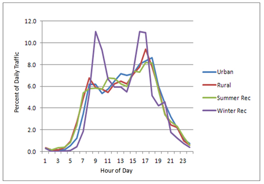
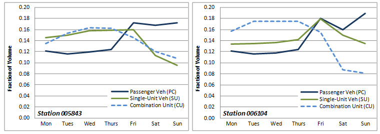
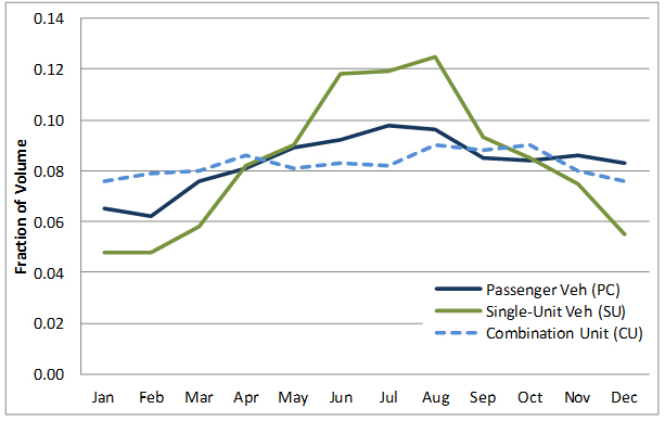
D. HOD Distribution – The repeatability of hourly variability is of great importance. Typical hourly variation in traffic volume on the traffic monitoring sites from Arizona DOT is shown in the figure below. The typical morning and evening peak hours are evident for urban routes on weekdays. The evening peak generally has somewhat higher volumes than the morning peak. Rural routes do not show two prominent peaks, while recreational routes shows a single daily peak (as travelers go to their recreational destination). Figure 3-3 shows an example of the HOD distribution.
Source: Federal Highway Administration.
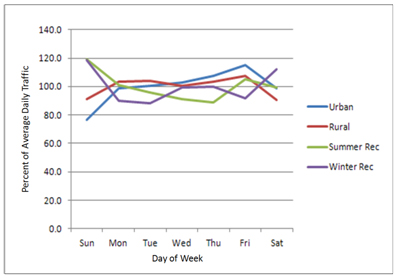
E. DOW distribution – Volume variation by day of the week is also related to site location (urban or rural) and the type of highway on which observations are made. Typical DOW variation in traffic volume on the traffic monitoring sites from Arizona DOT is shown in the figure below. Monday to Thursday traffic is similar and close to an average while the weekend traffic is generally lower than weekday traffic on urban routes. Friday traffic is generally higher than the rest of the days. States are allowed flexibility in how they design their DOW adjustment factor process to account most effectively for their own traffic patterns and data analysis process. At a minimum, weekday and weekend factors should be developed. However, individual DOW factors may be more appropriate in many cases due to the variability in traffic volumes from Friday through Monday on many roads.
Source: Federal Highway Administration.
If the factor groups are not reasonably homogeneous, the definition of the groups is not clear, or new traffic patterns are emerging, it may be necessary to re-form the monthly factor groups.
The basic statistic used to create factor groups can be either the ratio of AADT to MADT, or the ratio of AADT to MAWDT. In many States there are patterns of variation related to rural roads, urban roads, and recreational areas. However, in some States, significant geographic differences in travel need to be accounted for in the seasonal factoring process. For example, rural roads in the northern half of the State may have different travel patterns than rural roads in the southern half of the State. In addition, in some States clear patterns have failed to emerge.
The three prominent types of analysis are described as follows:
A. Traditional Approach – The more subjective traditional approach to grouping roads and identifying like patterns is based on a general knowledge of the road system combined with visual interpretation of the monthly graphs. The advantage of the traditional approach is that it allows the creation of groups that are easier for agency staff to identify and explain to users. This happens because the grouping process starts by defining road groups that are expected to behave similarly. The hypothesis is then tested by examining the variation of the seasonal patterns that occur within these expected groups.
The initial groups of roads that behave similarly could consist of roads of the same functional classification, or a combination of functional classifications. The groups should be further modified by the State highway agency to account for the specific characteristics of the State. Note that these are simply examples; there are other ways to accomplish this. Expected revisions include the creation of specific groups of roads that have travel patterns driven by large recreational activities, or that exhibit strong regional differences.
Deciding on the appropriate number of factor groups should be based on the actual data analysis results and the analyst’s knowledge of specific, relevant conditions. As a general guideline, a minimum of three to six groups is usually needed. More groups may be appropriate if a number of recreational patterns need to be monitored or if significant regional differences exist.
B.Cluster Analysis – The cluster procedure is illustrated by an example in Appendix G where the monthly factors (ratio of AADT to MADT) at the continuous count stations are used as the basic input to the statistical procedures. An understanding of the computer programs used for statistical clustering procedures is helpful but not required to interpret the program results
The cluster analysis procedures have two major weaknesses. One is the lack of theoretical guidelines for establishing the optimal number of groups. Determining how many groups should be formed is difficult. The cluster analysis process starts with all continuous counts in a single group, and proceeds until each continuous count is in an individual group. The difficulty is in determining at what point to stop this sequential clustering process. Unfortunately, the optimal number of groups cannot be determined mathematically.
The second weakness in the cluster analysis approach is that the groups that are formed often cannot be adequately defined, since the cluster procedure considers only variability at the continuous counts, not applicability to the short counts. Plotting the sites that fall within a specific cluster group on a map is sometimes helpful when attempting to define a given group output by the cluster process, but in some cases, the purely mathematical nature of the cluster process simply does not lend itself to easily identifiable groups.
Two advantages of cluster analysis are that it allows for independent determination of similarity between groups, therefore making the groups less subject to bias, and it can identify travel patterns that may not be intuitively obvious to the analyst. Accordingly, it helps agency staff investigate road groupings that might not otherwise be examined, which can lead to more efficient and accurate factor groups and provide new insights into the State’s travel patterns.
C. Volume Factor Groups – Because of the importance and unique inter-regional nature of travel on the interstate system, States should consider maintaining separate volume factor groups for the interstate functional categories. When interstate intrusive continuous count stations are not fiscally or logistically feasible, agencies utilize non-intrusive technologies to collect data. The interstate system will always be subject to higher data constraints because of its national emphasis and high usage levels. Most States maintain many continuous counts on the interstate system; therefore, separate interstate groups are easily created.
The following table shows the advantages and disadvantages of seasonal factor
| Type | Advantages | Disadvantages |
|---|---|---|
| Traditional | 1 – Creation of groups is easier 2 – Application for factoring can be explained 3 – Easier to assign short-term count to a group |
1 – May not stand statistical scrutiny |
| Cluster Analysis | 1 – Independent determination of similarity of groups without bias 2 – Traffic pattern can be found which may not be intuitively obvious 3 – Efficient and accurate factor groups |
1 – Lack of guidelines for establishing optimal number of groups 2 – Groups that are formed often cannot be adequately defined 3 – Difficult to assign short-term count to a group |
| Volume Factor Group | 1 – Consistent national framework for comparison among the State 2 – The precision of the seasonal factors can be calculated 3 – Easier to assign short-term count to a group |
1 – Functional or road classification may not be based on travel characteristics 2 – May not stand statistical scrutiny |
The TMG recommends the groups illustrated in Table 3-2 as a minimum
| Recommended Group | HPMS Functional Code |
|---|---|
| Interstate Rural | 1 |
| Other Rural | 2, 3, 4, 5, 6,7 |
| Interstate Urban | 1 |
| Other Urban | 2, 3, 4, 5, 6, 7 |
| Recreational | Any |
The first four groups are self-explanatory. The recreational group relies on subjective judgment and knowledge of the travel characteristics of the State. Usually, recreational patterns are identifiable from an examination of the continuous count data. The existence of a recreational pattern should be verified by knowledge of the specific locations and the presence of a recreational travel generator. A roadway is likely a recreational road when the difference between the ratio of the highest hourly volume to AADT and the ratio of the thirtieth highest hourly volume to AADT is greater than one. No single method exists for determining recreational patterns. A typical commuter pattern roadway can operate as a recreational pattern on weekends or a weekday depending on events, etc. The best way to determine trip purpose absolutely is to conduct intercept surveys.
Distinct recreational patterns cannot be defined based simply on functional class or area boundaries. Recreational patterns are obvious for roads at some locations but non-existent for other, almost adjacent, road locations. The boundaries of the recreational groups should be defined based on subjective knowledge. The existence of different patterns, such as for summer and winter, further complicates the situation. Therefore, the recommendation is to use a strategic approach to determine subjectively the routes or general areas where a given recreational pattern is clearly identifiable, establish a set of locations, and subjectively allocate factors to short counts based on the judgment and knowledge of the analyst. The road segments where these recreational patterns have been assigned should be carefully documented so that these recreational factors can be accurately applied and periodically reviewed
While this may appear to be a capitulation to ad hoc procedures, it is a realistic acknowledgment that statistical procedures are not directly applicable in all cases. However, recreational areas or patterns are usually confined to limited areas of the State and, in terms of total vehicle distance traveled (VDT), are small in most cases. The direct statistical approach will suffice for the majority of cases.
The procedure for recreational areas is then to define the areas or routes based on available data (as shown by the analysis of continuous and control data) and knowledge of the highway systems to subjectively determine which short counts will be factored by which continuous count (recreational) location. The remaining short counts should be assigned based on the groups defined by the State.
The minimum group specification can be expanded as desired by each State to account for regional variation or other concerns. However, more groups result in the need for more continuous count stations, with a corresponding increase in program cost and complexity. Each State highway agency will have to examine the trade-offs carefully between the need for more factor groups and the cost of operating additional continuous count stations.
The above definition of these seasonal patterns based on functional class provides a consistent national framework for comparisons among States and more importantly, provides a simple procedure for allocating short duration counts to the factor groups for estimating annual average daily traffic (AADT). It also provides a direct mechanism for computing the statistical precision of the factors being applied.
The precision of the seasonal factors can be computed by calculating the mean, standard deviation, and coefficient of variation of each adjustment factor for all continuous count locations within a group. The mean value for the group is the adjustment factor that should be applied to any short count taken on a road section in the group. The standard deviation and coefficient of variation of the factor describe its reliability. The error boundaries can be expressed in percentage terms using the coefficient of variation, where the error boundaries for 95 percent of all locations are roughly twice the coefficient of variation.
Typical monthly variation patterns for urban areas have a coefficient of variation under 10 percent, while those of rural areas range between 10 and 25 percent. Values higher than 25 percent are indicative of highly variable travel patterns, which reflect recreational patterns but which may be due to reasons other than recreational travel.
Having analyzed the data, established the appropriate seasonal groups, and allocated the existing continuous count locations to those groups, the next step is to determine the total number of locations needed in each factor group to achieve the desired precision level for the composite group factors. To carry out this task, statistical sampling procedures are used. Since the continuous count locations in existing programs have not been randomly selected, assumptions may be made. The basic assumption made in the procedure is that the existing locations are equivalent to a simple random sample selection. Once this assumption is made, the normal distribution theory provides the appropriate methodology. The standard equation for estimating the confidence intervals for a simple random sample is:
Where:
B = upper and lower boundaries of the confidence interval


n = number of locations
d = significance level
s = standard deviation of the factors
The precision interval is: 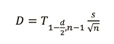
Where:
D = absolute precision interval
s = standard deviation of the factors
Since the coefficient of variation is the ratio of the standard deviation to the mean, the equation can be simplified to express the interval as a proportion or a percentage of the estimate.
The equation becomes: 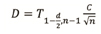
Where:
D = precision interval as a proportion or percentage of the mean
C = coefficient of variation of the factors.
Note that a percentage is equal to a proportion times 100, i.e., 10 percent is equivalent to a proportion of 1/10.
Estimating the sample size needed to achieve any desired precision intervals or confidence levels is possible using this formula. Specifying the level of precision desired can be a difficult undertaking. Very tight precision requires large sample sizes, which translate to expensive programs. Very loose precision reduces the usefulness of the data for decision-making purposes. Traditionally, traffic estimates of this nature have been considered to have a precision of plus or minus 10 percent. A precision of 10 percent can be established with a high confidence level or a low confidence level. The higher the confidence level desired, the higher the sample size required. Furthermore, the precision requirement could be applied individually to each seasonal group or to an aggregate statewide estimate based on more complex, stratified random sampling procedures.
The reliability levels recommended are 10 percent precision with 95 percent confidence for each individual seasonal group, excluding recreational groups where no precision requirement is specified. When these reliability levels are applied, the number of continuous count locations needed is usually five to eight per factor group, although cases exist where more locations are needed. The actual number of locations needed is a function of the variability of traffic patterns within that group and the precision desired; therefore, the required sample size may change from group to group.
Recreational factor groups usually are monitored with a smaller number of continuous counters, simply because recreational patterns tend to cover a small number of roads; it is not economically justifiable to maintain five to eight stations to track a small number of roads. The number of stations assigned to the recreational groups depends on the importance assigned by the planning agency to the monitoring of recreational travel, the importance of recreational travel in the State, and the different recreational patterns identified.
Once the number of groups and the number of continuous count locations for each group have been established, the existing locations can be modified if revision is necessary. The first step is to examine how many continuous counters are located within each of the defined groups. This number is then compared to the number of locations necessary for that group to meet the required levels of factor reliability. If the examination reveals a shortage of current continuous count locations, the agency should select new locations to place continuous counters within that defined group. Since the number of additional locations may be small, the recommendation is to select and include them as soon as possible. Additional issues that should be considered when selecting locations to expand the sample size are reviewed in the following paragraphs.
If a surplus of continuous counters within a group exists, then redundant locations are candidates for discontinuation unless needed for ramp balancing and anchors. If the surplus is large, the reduction should be planned in stages and after adequate analysis to ensure that the cuts do not affect reliability in unexpected ways. For example, if 12 locations are available and six are needed, then the reduction could be carried out by discontinuing two locations annually over a period of three years. The sample size analysis should be recomputed each of the three years before the annual discontinuation to ensure that the desired precision has been maintained. Location reductions should be carefully considered. Maintaining a few (two to three) additional surplus locations may help supplement the groups and compensate for equipment downtime or missing data problems.
Matters for consideration are as follows:
MOY factors are most accurately developed and applied on a year-by-year basis. That is, a short count taken in 2009 should be adjusted with factors developed exclusively from continuous count data collected in 2009. This allows the adjustment process to account for economic and environmental conditions that occurred in the same year the short count was taken.
This recommendation creates problems for the timing of factor computation and application. That is, if a short count is taken in the summer of this year, the true adjustment factor for this year cannot be computed until January of next year at the earliest, which may not be timely enough for many users. The recommendation is to compute temporary adjustment factors for estimating AADT before the end of the year, and then to revise that preliminary estimate once the year’s true adjustment factors can be computed in January.
Temporary factors can be developed in one of three ways:
The first of these approaches is the easiest but also the least accurate, because the effects of this and last years’ economic/environmental conditions are likely to be different. The second approach reduces the biases that occur from using a single year’s factors. The last approach produces the most accurate adjustment factor but also requires the most labor-intensive data handling and processing effort. (See Appendix D, Case Study #6 for an example of computing monthly rolling average.)
The procedures for developing and using monthly factors to adjust short volume counts to produce AADT estimates follow directly from the structure of the program. The individual monthly factors for each continuous count station are the ratio of the AADT to MADT. Alternatively, the State can combine the DOW adjustment and monthly adjustment into a single factor, for example the ratio of annual average daily traffic to monthly average weekday traffic (AADT / MAWDT). This term, or a similar seasonal adjustment, can be substituted directly for the ratio of AADT / MADT in the factor grouping and application process if desired.
For a counter site that operates 365 days per year without failure, the AADT can be computed by adding all of the daily volumes and dividing by 365. Similarly, the MADT can be computed by adding the daily volumes during any given month and dividing by the number of days in the month.
Challenges with this approach are that few continuous count stations operate reliably during any given year. Most suffer at least small amounts of downtime because of power failures, communications failures, and other equipment or data handling problems. These missing hours or days of data can cause biases and other errors in the calculations, particularly when a moderate amount of data is lost in a block. As a result, a modified formula for computing these types of statistics that directly accounts for missing data has been adopted.
The following methodology has been adopted by AASHTO, has been researched and verified by FHWA, is used by many States, and is recommended by FHWA.

Where:
VOL = daily traffic for day k, of DOWi, and month j
i = day of the week
j = month of the year
k = 1 when the day is the first occurrence of that day of the week in a month, 4 when it is the fourth day of the week
n = the number of days of that day of the week during that month (for which you have data
This formula computes an average DOW for each month, and then computes an annual average value from those monthly averages, before finally computing a single annual average daily value. This process effectively removes most biases that result from missing days of data, especially when those missing days are unequally distributed across months or days of the week. The method used should be detailed in the Traffic Monitoring System (TMS) that States keep on record with the local FHWA district office.
The calculation of MADT is similar to that of AADT. An average DOW is first computed for a given month, and then all seven-day values are averaged. MAWDT is similarly computed. However, each State can define the specific days present in the MAWDT calculation. For example, some States do not count Fridays for routine short duration traffic counts and therefore, choose not to include Fridays in the computation of MAWDT.
Monthly factors for each continuous count are computed by the ratio of AADT to MADT or AADT to MAWDT. Group monthly factors are computed as the average of the factors for all continuous counter locations within the group. Both the individual continuous count and the group factors should be made available to users in tabular and computer accessible form. (See Appendix K for examples of these computations. See Appendix D, Case Study #5 for an example from Alabama regarding incorporating data collected by local governments.)
Measurements of vehicle speeds are used for a wide variety of studies, but particularly for safety studies and roadway performance monitoring. The data needed for these two types of studies are highly related but can be significantly different in both content and format. Safety studies rely on statistically valid measures of vehicle speed distributions during the study periods. Of particular interest in most safety studies is the speed distribution that occurs under free flow conditions (e.g., how many vehicles are speeding and how fast are they going? Is there a large difference in speed between the fastest and slowest vehicles in the traffic stream?). On the other hand, those conducting roadway performance monitoring are more interested in how the average speed of the facility changes by time of day and from one day to the next (e.g., is congestion forming, and if so, how often, how badly, and how long does it last?).
Consequently, speed data for most safety studies are gathered with traditional traffic monitoring devices, which collect speed data for all vehicles passing a selected point in the roadway over a defined period. Speeds are then reported either as individual vehicle observations or as summary data that indicate the volume of vehicles moving within defined speed ranges (speed bins).
Conversely, speed data for performance monitoring purposes traditionally come from sensors used for traffic management purposes. Average facility speeds are the primary reporting statistic calculated with data from these sensors, and individual vehicle speeds are often not collected. Recent decreases in the cost of both GPS equipment and wireless communications costs have also meant that privately collected vehicle probe data sets can now also meet many performance-monitoring needs. Unfortunately, these probe vehicle data only include a small sample of vehicles using a roadway, which can be used to estimate average facility speeds along entire roadway corridors across all days of the year. These data sets are less useful for most safety studies because they do not capture an unbiased measure of the distribution of speeds.
This edition of the TMG provides guidance on the collection and submission of speed data that are of particular use for safety studies. It does not contain guidance on the collection and use of vehicle probe based speed data useful for more general, area-wide, or corridor long roadway performance monitoring.
Travel speed data is used to determine travel time reliability, and is important for planning, program effectiveness evaluation, and investment analysis. Many other divisions within State DOTs need speed data for travel time, performance measures, safety studies, and other analysis. Multiple divisions within an agency could consider funding a permanent site, collecting the data once and using it many times across divisions/agencies.
Many continuous traffic-monitoring devices are deployed specifically to collect vehicle speed data; others collect speed data as a by-product of some other traffic data collection function. By taking advantage of all of their devices collecting speed data—whether intentionally or as a by-product—highway agencies frequently have access to a wealth of vehicle speed data. Many continuous counters are equipped with dual loops simply because the cost of the second loop is low in comparison to the initial investment at that site, and the provision of the second loop both provides redundancy in volume data collection and allows that location to be used for other purposes (speed monitoring and length classification).
The deployment of continuous equipment specifically to collect vehicle speed data is becoming popular in States. In an effort to leverage the capabilities of the current equipment, FHWA investigated speed data collection practices of States and found that 94 percent have speed data; all of the States collect speed data themselves, and five of the States use third parties to collect speed data.
Chapter 5, Transportation Management and Operations discusses ideas for sharing resources with other offices to collect speed data.
Data already collected at States are as follows:
This flexible structure would enable the reporting of spot speed without changing the data collection methodology currently being used by States. The final format for submission is identified in Chapter 7.
A well-designed monitoring program stores, summarizes, and makes available the speed data already collected by these devices for both internal agency use and submittal to U.S. DOT.
This section discusses the process for establishing a continuous vehicle classification count program and presents two alternative methods for the development of factor groups for classification. The continuous vehicle classification data collection program is related to, but can be distinct from, the traditional continuous count program. In addition, factoring of vehicle classification counts (i.e., heavy vehicle volume counts) may be performed independently from the process used to compute AADT from short duration volume counts. Highway agencies should collect classification data (which also supply total volume information) in place of simple volume counts whenever possible.
Figure 3-5 shows the steps for the classification process and are explained in the following paragraphs.
FOR DEVELOPING AND USING KNOWLEDGE OF THE TRAFFIC PATTERNS FOR EACH CLASS OF VEHICLE
Source: Federal Highway Administration.
A. Current Program – The first step in developing the continuous vehicle classification count program is to define, analyze, and document the current program. This assessment should include the historical design, procedures, equipment, personnel, objectives, and uses of the information. This review should begin with an inventory of the State’s continuous vehicle classification data collection equipment. The uses of the data should be identified, as well as who is using it and how it might be used if additional application tools were available
B. Traffic Patterns – The data should be reviewed to determine what unique traffic patterns exist for each major classification of vehicle in the State and whether previously identified patterns have changed in order to establish whether the monitoring process should be adjusted.
C. Data Adjustment – The details of the data adjusted/processed should be reviewed with attention to whether the data adjustment steps can be improved or otherwise made more efficient. Of considerable interest in this review is how the quality of the data being collected and reported is maintained. Establishing the quality of the vehicle classification data reported and the outputs of the data analysis process is a prerequisite for future improvements. Continuous traffic data collection is subject to discontinuities due to equipment malfunctions and errors. The way a State identifies and handles errors in the data stream is a key component of the vehicle classification program. Subjective editing procedures for identifying and imputing missing or invalid data is discouraged, since the effects of such data adjustments are unknown and may bias the resulting estimates. Instead, the quality control procedures listed below should be followed to ensure that invalid data is appropriately and consistently identified and replaced.
D. Quality Control – Each State highway agency should have formal rules and procedures for these important quality control efforts. The implementation of truth-in-data concepts as recommended by the AASHTO Guidelines for Traffic Data Programs will greatly enhance the analytical results and help in establishing objective data patterns. Truth-in-data implies that agencies maintain a record of how data is manipulated, and that each manipulation has a strong basis in statistically rigorous analysis. Data should not be discarded or replaced simply because they appear atypical. Instead, each State should establish systematic procedures that provide the checks and balances needed to identify invalid data, control how those invalid data are handled in the analysis process, and identify when those quality control steps have been performed
E. Finally, the State highway agency should periodically review whether these procedures are performed as intended or need to be revised. For States that currently do not have formal quality control procedures, Appendix E provides several examples of how States use data quality control procedures. In addition, AASHTO has also provided guidance on how to develop and implement a quality control process for traffic data collection.
F. Summary Statistics – The last portion of the review process should entail the steps for creating summary statistics from the raw data collected by vehicle classification equipment. These procedures should be consistent and should accurately account for the limitations that are often present in continuously collected classification data.
Correctly manipulating continuous vehicle classification count data after they have been collected is vital.
A. Existing Data Sources – The inventory of existing (and planned) continuous vehicle classification ensures that the State’s traffic monitoring effort is comprehensive and effective. As noted earlier, the key to the inventory process is for the agency to identify not only the traditional continuous vehicle classification, but also other data collection devices that can supply continuous class data. These secondary sites include, but are not limited to:
B. When available, data collection devices operated by the same group that operates the vehicle classification sites are the easiest from which to obtain data, but a number of State highway agencies do not make use of this data as part of their vehicle classification process.
C. Other Sources – Posing more challenges are devices operated by other divisions within the State highway agency. Obtaining this data can be difficult, particularly when internal cooperation within the agency is limited. However, the current emphasis on improved cost-efficiency in government means that in most States there is strong upper management support for full utilization of data resources, wherever they exist. The key to taking advantage of this support is to make the transfer of the data as automated as possible, so that little or no staff time is expended outside of the traffic data collection group to obtain the data.
D.The State highway agency should also seek data outside of its own agency. (See Chapter 5, case study examples.) While it may not be possible to obtain this data at the level provided by continuous vehicle classification equipment, it is often possible to obtain useful summary statistics from these locations. These summary data can be used to supplement the State’s data at those locations and geographic areas. The availability of data from supplemental locations reduces the cost of collecting and increases access to useful data. To obtain this data, the State highway agency may have to acquire software that automatically collects and reports this data. The intent, once again, is to reduce the operating agency’s staff time needed to collect and transmit the data. The easier this task is for the agency collecting the data, the more likely it is that this data can be obtained. However, data should only be used from calibrated sites (all sites including classification should be calibrated yearly).
E. Uses of Data – Another element is to inventory data uses and users. This step involves determining how the vehicle classification data is currently being used, who the customers are for those data, and which data products are being produced. Data should be collected for a purpose, and the users and uses of those data should be prioritized. Data only have value when they answer important questions. By understanding how the data is being used, it is possible to develop a clear understanding of what value the data collection effort has to the organization. Understanding this value, and being able to describe it, is crucial to defending the data collection program when budget decisions are made.
F. States should be checking the accuracy of their class data and taking appropriate action to evaluate and adjust their vendor-specific classification algorithm to correctly classify all of the vehicle types on their roadways (within 10% by class).
G. This inventory process may uncover the circumstance that some data and/or summary statistics are not being used. If that is the case, then those data and statistics may be eliminated in favor of the collection of data or production of statistics that will be used. This results in better use of available resources, makes the data collection system more focused on products actively desired by agency users, and results in more support for the data collection program from others in the agency. Several State DOTs find the use of a data business plan to be a useful tool for documenting the business needs for data and information (Chapter 2). Data business plans help to document how data systems support current business operations, identify data gaps (i.e., where new data and information are needed to support current needs), and provide a structured plan for the development of enhanced data systems to meet future needs.
If sufficient data is available, it should be evaluated to determine what unique traffic patterns exist for each of the different classes of vehicles. For example, motorcycles have different DOW and monthly travel patterns than single unit trucks. The development of factor groups and factor procedures for different classes of vehicles should be undertaken. At a minimum, States should investigate whether they need different factor groups and processes for six aggregate classes of vehicles: motorcycles (MC), passenger cars (PV), light duty trucks (LT), buses (BS), single unit trucks (SU), and multi-unit combination trucks (CU). In some cases, two or more classes of vehicles may be included in one set of factors when these vehicles can be shown to have similar travel patterns.
The inventory process should document whether and how the continuous vehicle classification program is being used to create and apply adjustment factors to short duration vehicle classification traffic counts to estimate annual average volumes by type of vehicle. The inventory review process should also determine which highway locations require continuous vehicle classification equipment to capture the travel patterns effectively of all vehicle classes with a high degree of confidence.
The review of seasonal patterns can be undertaken using one of a number of analytical tools. Two of the most useful are cluster analysis, which can be performed using any one of several major statistical software packages such as SAS or SPSS, and the graphic examination, using GIS tools, of seasonal pattern data from individual sites.
The intent of the seasonal pattern review is to assess the degree of seasonal (monthly) variation that exists in the State as measured by the existing vehicle classification data and to examine the validity of the existing factor grouping procedures that produce the seasonal factors. The review consists of examining the monthly variation (attributed to seasonality) in vehicle traffic volume for each class of vehicles (at a minimum of MC, PV, BS, LT, SU and CU) at the existing vehicle classification locations, followed by a review of how roads are grouped into common patterns of variation. The goal of this review is to determine whether the State’s procedures successfully group roads with similar seasonal patterns, and whether individual road segments can be correctly assigned to those groups.
It is not necessary for the factor groups to be identical to the cluster analysis output for two reasons. For any given year, the cluster output is likely to be slightly different, as minor variations in traffic patterns are likely to be reflected in minor changes in the cluster analysis output. In addition, the cluster analysis output will require adjustment to create intuitively rational and identifiable groups of roads. The use of cluster analysis is explained in further detail in Appendix G.
The remaining review step is to make sure that the groups are defined by an easily identifiable characteristic that allows easy assignment of short counts to the group. The definition of each group must be complete enough to allow analysts to select the appropriate factor for every applicable roadway section.
Each State highway agency should operate a set of continuous classification counters to measure vehicle-travel patterns and provide the factors to convert short classification counts to annual averages. As an example of one vehicle type, research has shown that truck travel does not follow the same time-of-day, DOW, and seasonal patterns as total volume (Schneider and Tsapakis 2009, Hallmark and Lamptey 2004, Hallenbeck and Kim 1993, Weinblatt 1996, Hallenbeck et al 1997). For example, see Figures 3-6 and 3-7 below.
Analysis of continuously collected data sets also indicates that truck volumes on many roads (even high volume interstate) can change significantly due to changes in the national and local economy. Similarly, continuous count data have shown that motorcycle traffic follows different patterns than other passenger vehicles with much more travel occurring on weekends than weekdays, especially on some rural roads used for recreational travel by motorcyclists. Continuously operating classification counters are needed to monitor these travel patterns so that these patterns can be detected and accounted for in engineering and planning analyses. For example, if the large increases in weekend motorcycle travel are not accounted for, short duration classification counts will significantly underestimate the number of miles traveled annually on motorcycles, thus biasing national and State safety analyses.
Source: Federal Highway Administration
Source: Federal Highway Administration
All State highway agencies have been operating permanently installed continuous count stations (CCS) (commonly referred to as ATRs) for many years. It has only been since the mid-1980s that technology allowed the installation and operation of similar counters to collect continuous classification data. A significant increase in the number of these counters has taken place since 1990 because of the start of traffic data collection for the Strategic Highway Research Program’s (SHRP) Long Term Pavement Performance (LTPP) project. Many States have also converted continuous installations to classification as the old equipment was replaced.
Data from these continuous classification devices have shown that motorcycle, single unit truck, and combination unit truck volumes have time-of-day, DOW, and by month variations that are different from those of cars. In addition, sources of continuous classification data may be obtained from installations from regulatory, safety, and traffic management systems installed to operate and manage the infrastructure. To obtain these existing data, highway agencies often need to establish working relationships with other public agencies, including MPOs, county and regional planning councils, to coordinate count programs and sharing of data. The effort may result in considerable improvement to the available classification data. FHWA is working on establishing length-based classification (see Appendix J, FHWA Memo on Establishing Length Based Classification).
The objective of seasonal factor procedures is to remove the temporal bias in current estimates of vehicles with unique temporal variances that are different from the total volume. Four primary reasons for installing and operating permanent, continuously operating, vehicle classifiers for traffic monitoring purposes include the ability to:
Regardless of the approach taken for the computation and application of factors, it is recommended that adjustment factors be computed for a maximum of six generalized vehicle classes (see VM-1 and HPMS Summary types). These are:
Table 3-3 compares the six-vehicle class groupings used in one of the HPMS datasets to the FHWA 13 vehicle category classes.
| HPMS Summary Table Vehicle ClassGroup* | FHWA 13 Vehicle Category Classification Number |
|---|---|
| Group 1: Motorcycles (MC) | 1 |
| Group 2: Passenger Vehicles equal to or under 102” (PV) | 2 |
| Group 3: Light trucks over 102” (LT) | 3 |
| Group 4: Buses (BS) | 4 |
| Group 5: Single-unit vehicles (SU) | 5,6,7 |
| Group 6: Combination Unit (CU) | 8,9,10,11,12,13 |
* These groupings are used to report travel activity by vehicle type in the Vehicle Summaries dataset for HPMS.
Highway agencies may adjust these categories to reflect their vehicle fleets and travel patterns best, as well as the capabilities of the classification equipment in their programs. (Note that where data shows similar patterns, the passenger car and light truck categories can be combined into one set of factor groups.)
Several reasons support these recommendations. The factoring process does not work well with low traffic volumes. With low volumes, even small changes result in high-percentage changes that make the computed factors highly unstable and unreliable. Even on moderately busy roads, many of FHWA’s 13 category vehicle classes (illustrated in Appendix C) will have mathematically unstable vehicle flows simply because their volumes are low. Aggregating the vehicle classes provides for more stable and reliable factors.
A second reason is that computing factors for the individual 13 vehicle classes may introduce too much complexity. There is no gain in separately annualizing extremely variable and rare vehicle classification categories.
Some issues presenting challenges to the factor development and application process remain unanswered, such as adequate editing procedures, resolution of the assignment of vehicles to classification categories, inability of equipment to collect a standard set of vehicle classes in all conditions, and disparities in the available equipment. Unnecessary complications at this stage of development should be avoided.
The following alternative truck volume factor procedures both have advantages and disadvantages. Both are complementary and can be combined as appropriate. States are encouraged to develop these alternative factor procedures or other alternatives that effectively remove temporal bias
The first procedure involves the use of roadway-specific factors. The second is an extension of the traditional traffic volume factoring process involving the creation of groups and the development of average factors for each of the groups.
Either applying factors to a road or fitting road segments into groups involves making decisions to resolve difficulties. A factor process may result in one set of factors for cars, another set of factors for trucks, and the combination of both to arrive at a total volume. A factor process may also require more than one set of factors for trucks where different truck types are factored separately. Some roads could conceivably fit in one factor group for cars, a second factor group for single unit trucks, and a third factor group for combination trucks. Resolutions should be made by each State between the need for accuracy and reductions in unnecessary complexity in the approach to removing temporal bias.
Two basic elements to the factoring process are the computation of the factors to apply to the short counts and the development of a process that assigns these factors to specific counts taken on specific roadways. The roadway-specific and the traditional procedures approach these two aspects of the factoring process differently. The result is two different mechanisms for creating and applying factors, each with its own strengths and weaknesses.
One option is the process that was developed by the Virginia Department of Transportation (VDOT) in the late 1990s. VDOT operates continuous counters on all major roads and the counters are used to develop road-specific factors. A short classification count taken on a specific road is adjusted using factors taken from the nearest continuous classification counter on that road. A factor computed for a specific road is not applicable to any other road.
As a result, a continuous classification counter should be placed on every road for which an adjustment factor is needed. This requires a large number of continuous vehicle classification counters and substantial resources. However, it ensures that a road can be directly identified with an appropriate factor and provide considerable insight into the movement of freight and goods within the State. The rule for assigning factors to short counts is simple and objective.
Identifying a specific road with a specific factor removes a major source of error in the computation of annual traffic volumes by removing the spatial error associated with applying an adjustment factor. Further, it produces factors that are applicable to all trucks using that road. The fact that different truck classes (single-unit versus combination trucks) exhibit different travel patterns is irrelevant, since all patterns are computed for that road. Having road-specific continuous classification counters also greatly reduces the number of short duration counts that are needed, since the continuous counters provide classification data for road sections near the count locations. The quality of data from continuous classification counters is superior to that of short counts.
Finally, this approach has the advantage of simplifying the calculation of adjustment factors, the application of those factors, and the maintenance of the program. For example, there is no need to develop groups and the application is performed one road at a time. Problems with continuous counters only apply to the affected roads and prioritization of counter problem correction can be based on road priority.
The most important disadvantage with this approach is cost. It is expensive to install, operate, and maintain large numbers of continuous traffic counters. The larger the system to be covered, the larger the cost. Even for smaller States, the cost to install a large counter base may be prohibitive. However, this approach may apply effectively to the interstate, where sufficient continuous counters may be available. It can also be applied to roads where current counters are installed.
A second disadvantage is that many roads are quite long and the character of any given type of vehicle traffic over their length can change drastically. This is why short count short duration programs are valuable. An adjustment factor taken on a road segment may not be applicable to another segment a few (two to three) miles down the road, particularly if a significant vehicle generation activity takes place along that stretch of roadway. Traffic patterns change because of economic activity, traffic generators, or road junctions. Not only does this further increase the number of continuous counters required, it also creates difficulty in selecting between the two continuous classification counters when a short count falls in between.
That is, specific road factors may be used for the most important truck roads and the traditional factor groups for routes without continuous classification counters. When continuous counters fail, traditional factoring techniques can then be used to provide adjustment factors on those roads. This combination of the traditional and roadway-specific factors may be an effective compromise between these two techniques
One final consideration with the roadway-specific technique is that there is no mathematical mechanism that allows computation of the accuracy/precision of the factors as they are applied to a given roadway section. Caution is recommended when significant traffic generators in the intervening space between the count and the continuous counter exist. When these factors are applied to count locations that are close to the continuous counter, they can be assumed to be quite accurate. However, as the distance between the short count and the continuous counter grows, and particularly as more opportunity exists for trucking patterns to change, the potential for error in the factor being applied grows, and at an unknown (but potentially substantial) rate.
The traditional factor process involves categorizing roads that have similar individual vehicle traffic patterns. A sample of data collection locations is then selected from within each group of roads, and factors are computed and averaged for each of the data collection sites within a group. A definition is provided for each group to describe characteristics that explain the observed pattern, which is used to allow the objective assignment of short counts to the groups. For example, a group might be defined as all roads in counties that experience heavy beach traffic, as these roads have unique seasonal and DOW recreational traffic. Similarly, for truck factors a logical grouping might be all roads serving heavy north/south or east/west through trucking movements, versus those roads that serve primarily local delivery movements.
For traffic volume, the traditional characteristics for grouping roads have been the functional class of the road (including urban or rural designation) and geographic location within the State. These groups are then supplemented with an occasional recreational (or geographic) designation for roads that are affected by large recreational traffic generators.
This same technique can be applied to truck traffic patterns. However, the characteristics that need to be accounted for can be different. Functional class of roadways has been shown to have an inconsistent relationship to truck travel patterns (Hallenbeck et al 1997, Schneider and Tsapakis 2009). Instead, truck travel patterns appear to be governed by the amount of long distance truck through-traffic versus the amount of locally oriented truck traffic, the existence of large truck traffic generators along a road (e.g., agricultural or major industrial activity), and the presence or absence of large populations that require the delivery of freight and goods. Understanding how these and other factors affect truck traffic is the first step toward developing truck volume factors. Developing this understanding requires analysis of the existing continuous vehicle classification data already being collected by the State, and analyzing it within the context of the commodity movements happening in the State. The steps required to gain this understanding are described below.
The creation and application of adjustment factor groups (time of day, DOW, and monthly) by class of vehicle is a topic that is still new. Most State DOTs have yet to develop these factoring procedures, and considerable research still needs to be accomplished.
States should depend on available classification data and knowledge to begin the development of truck traffic patterns. Truck traffic patterns are governed by a combination of local freight movements and through-truck movements. Extensive through-truck movements are likely to result in higher night truck travel and higher weekend truck travel. Through-traffic can flatten the seasonal fluctuations present on some roads while creating seasonal peaks on other roads not associated with the economic activity occurring in the land abutting that roadway section. Similarly, a road primarily serving local freight movements will be highly affected by the timing of those local freight movements. For example, if the factory located along a given road (not subject to significant amounts of through-traffic) does not operate at night, there may be little freight movement on that road at night.
Functional road classification can be used to a limited extent to help differentiate between roads with heavy through-traffic and those with only local traffic. Interstates and principal arterials tend to have higher through-truck traffic volumes than lower functional classes. However, there are interstates and principal arterial highways with little or no through-truck traffic, just as some roads with lower functional classifications can carry considerable through-truck volumes. Therefore, functional classification of a road by itself is a poor identifier of truck usage patterns. To identify road usage characteristics, additional information should be obtained from either truck volume data collection efforts or the knowledge of staff familiar with the trucking usage of specific roads. The truck volume data patterns, especially time of day patterns from short counts and DOW and monthly patterns from continuous classifiers, identify travel patterns for different types of vehicles. These patterns should then be discussed with staff working on freight planning activities to understand and help identify trucking patterns in ways that allow both grouping of continuous counters and assignment of short count location to those groups.
Among the types of patterns that can be identified through this combination of data and communication with staff are various local, regional, and through travel patterns. For example, local truck traffic can be generated by a single facility such as a factory, or by wider activity such as agriculture or commercial and industrial centers. These point or area truck-trip generators create specific seasonal and DOW patterns, much as recreational activity creates specific passenger car patterns. Truck trips produced by these generators can be highly seasonal (such as from agricultural areas) or constant (such as flow patterns produced by many types of major industrial plants). Where these trips predominate on a road, truck travel patterns tend to match the activity of the geographic point or area that produces those trips. In addition, changes in the output of these facilities can have dramatic changes in the level of trucking activity. For example, a labor problem at a West coast container port may produce dramatic shifts in container truck traffic to other ports. This results in significant changes in truck traffic on major routes serving those ports. Expansion or contraction of factory production at a major automobile plant in the Midwest can cause similar dramatic changes on roads that serve those facilities.
Truck trip generators can also affect the types of trucks found on a road. Specific commodities tend to be carried by specific types of trucks. However, State-specific truck size and weight laws can mean that trucks typical in one State may not be common in others. For example, multi-trailer trucks are common in most western States, while they make up a much smaller percentage of the trucking fleet in many eastern States. Understanding the types of trucks used to carry specific commodities is critical to understanding the trucking patterns on a road and how those patterns are likely to change (e.g., coal trucks in Kentucky and Pennsylvania).
Many other elements affect truck travel. For example, construction trucks operate in an area’s roads until the construction project is completed and then they move somewhere else. This type of truck movement is difficult to quantify. Roads near truck travel generators, such as quarries or trash dumps, carry consistent truck traffic and the type of truck is well known. Summarizing the different patterns in a way that allows creation of accurate factor groups is difficult. Obviously, the more knowledge that exists about truck traffic on a road, the easier it is to characterize that roadway.
Geographic stratification and functional classification can be used to create truck factor groups that capture the temporal patterns and are reasonably easy to apply. An initial set of factor groups might look something like that shown in Table 3-4. However, the two keys to the creation of groups is that the data should show that traffic patterns within grouped sites are in fact similar, and those groups should be designed in such a manner that short counts can be easily and accurately assigned to the correct factor groups. Therefore, as groups are formed, specific roads may need to move from one group to another to ensure that both of these constraints remain true.
Definitions like those above group roads with as homogenous truck travel patterns as possible, and provide easy identification of the groups for application purposes. They present a starting point to begin the identification process necessary to form adequate groups.
Performing a cluster analysis using truck volumes (as illustrated in Section 3.2.1 for total volume) will help to identify the natural patterns of variation and to place the continuous counters in variation groups. This will help in identifying which groups may be appropriate and in determining of how many groups are needed. One of strengths of the cluster analysis is that it identifies groups only by variation. The weakness is that it does not describe the characteristics of the group that allow application of the resulting factors to other short counts. The example definition in Table 3-2 does exactly the opposite. It clearly establishes group characteristics but cannot indicate whether the temporal variation is worth creating separate groups or not. As is the case for AADT group procedures, a combination of statistical methods and knowledge should be used to establish the appropriate groups.
| Rural | Urban |
|---|---|
| Interstate and arterial major through-truck routes | Interstate and arterial major truck routes |
| Other roads (e.g., regional agricultural roads) with little through traffic | Interstate and other freeways serving primarily local truck traffic |
| Other non-restricted truck routes | Other non-restricted truck routes |
| Other rural roads (e.g., mining areas) | Other roads (non-truck routes) |
| Special cases (e.g., recreational, ports) | |
All roads within the defined factor groups should have similar types of vehicle volume patterns. To verify this condition, the continuous counter data available within the groups should be examined. For each continuous classification counter in a group, compute the temporal adjustment factors of interest (DOW, month, or combined) for each of the vehicle types desired, and then compute the mean and standard deviation for the group as a whole. Plots of the volumes and the factors over time can also help to determine whether the travel patterns at the continuous sites are reasonably similar.
In most cases, only a few roads within each group will have sufficient data (continuous classification counters) needed to estimate travel patterns. The assumptions this analysis makes are similar to those made for AADT factors. The implication is that the continuous counters typify the existing temporal variation. Then the continuous counter variation reflects the variation existing at locations where no continuous counters exist. A combined monthly and weekday factor is computed as follows (This formulation assumes a multiplicative application. AADTT is equal to the average 24-hour count times the adjustment factor. Many States use the inverse of this formula and apply the resulting factor by dividing the average 24-hour volume obtained from their short count by the adjustment factor. See Table 3-9 for example):
An example of how these monthly adjustment factors differ by vehicle class is shown below in Table 3-5.
| MC | Car and Light Trucks | Buses | Single Unit Trucks | Combination Trucks | Total Volume | |
|---|---|---|---|---|---|---|
| MADTVehicle_Class | 35 | 4,874 | 52 | 227 | 1,639 | 6,826 |
| AADTVehicle_Class | 33 | 5,499 | 57 | 288 | 1,653 | 7,530 |
| Monthly Factor(AADTc/MADTc) | 0.95 | 1.13 | 1.10 | 1.27 | 1.01 | 1.10 |
Computing the mean (or average) for the June factor for all sites within the factor group yields the group factor for application to all short counts (weekdays in June) taken on road segments within the group. The standard deviation of the factors within the group describes the variability of the group factor. The variability can be used to determine whether a given factor group should be divided into two or more factor groups, to compute the precision of the group factor, and to estimate the number of continuous classification counter locations needed to compute the group factor within a given level of precision. An example of this is in Table 3-9.
The variability of each statistic computed for the factor group will have a different level of precision. For example, the June factor will have different precision than the July factor. The precision will also vary for each of the vehicle types analyzed.
The information on variability must be reviewed to determine whether the roads grouped together have similar individual vehicle travel patterns. A number of methods can be used to determine whether various sites belong together. A statistically rigorous approach to testing the precision of the selected groups requires the use of fairly complex statistics, an examination of all the truck classes used, and the comparison of statistical reliability for all the different types of statistics produced, with the reliability users need for those statistics. This is a complex and difficult analysis. The analysis can be simplified by concentrating on the most important vehicle classes and statistics produced. However, even with the simplifications suggested, trade-offs are necessary. No designed group will be optimal for all purposes or apply perfectly to all sites. For example, in one group of roads, the single tractor-trailer volumes on roads within each group may have similar travel characteristics, but the single-unit truck volume patterns are quite different from each other. By changing the road groups, it may be possible to classify roads so that all roads have similar travel patterns for single-unit trucks, but then the single tractor-trailer patterns become highly variable.
At some point, the analyst will need to determine the proper balance between the precision of the group factors developed for these two classes of trucks, or they will have to accept different factor groups for different vehicle classes. Each road may end up in multiple factor groups depending on what vehicle classification volume is being factored. Use of multiple groups may result in a more accurate factor process but will certainly result in a more complicated and confusing procedure.
The trade-offs between alternative factor groups can only be compared by understanding the value of the precision of each statistic to the data user. In most cases, this is simply a function of determining the relative importance of different statistics. For example, if 95 percent of all trucks are single tractor-trailer trucks, then having road groups that accurately describe tractor-trailer vehicle patterns is more important than having road groups that accurately describe single-unit truck patterns. Similarly, if single-unit trucks carry the predominant amount of freight (this occurs in mineral extraction areas), then the emphasis should be on forming road groups that accurately measure single-unit truck volume patterns.
The quality of a given factor group can be examined in two ways. The first is to examine graphically the traffic patterns present at each site in the group. Figure 3-8 is an example of a set of monthly truck volume patterns for a group of sites in Washington State that could be considered a single factor group. Graphs like these give an excellent visual description of whether different data collection sites have similar travel patterns. The second method is to compute the mean and standard deviation for various factors that the factor group is designed to provide. If these factors have small amounts of deviation, the roads can be considered to have similar characteristics. If the standard deviations are large, the road groupings may need to be revised.
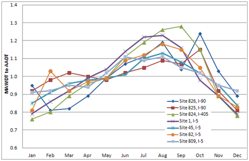
Source: Federal Highway Administration.
An estimate of the precision of the group factor can be derived from the standard deviation. For example, the precision of the June adjustment factor computed above can be estimated using the standard deviation of that estimate. The precision of the group factor can be estimated with 95 percent confidence as approximately plus or minus 1.96 times the standard deviation divided by the square root of the number of sites in the group. (This is a relatively crude approximation because it assumes that the standard deviation calculated from the seven sample sites is equal to the actual standard deviation of the population of the group of roads. The value 1.96 should be used only for sample sizes of 30 sites or more. A more statistically correct estimate would use the student’s t distribution, which for six degrees of freedom (seven classification sites) is 2.45. The calculation also assumes that the factors are normally distributed and that sites are randomly selected.)
Increasing the number of continuous counter locations within a group will improve the precision of the group factor. However, increasing the number of continuous classification counter locations only marginally improves the precision of the group factor application at specific roadway sections. That is, increasing the sample size makes the group factor itself a better measure of the mean for the group, but the mean value may or may not be a good estimate of the pattern at any given roadway section within that group. The standard deviation of the group factor measures the diversity of the site factors within the group.
There can be cases where the factors will not improve the annual volume estimates, particularly in high variability situations. An alternative is to take multiple site-specific classification counts at different times during the year to measure seasonal change. This can be an effective way to estimate annual individual vehicle traffic accurately for high profile projects that can afford this additional data collection effort. This alternative can also be used to test the accuracy of the annual estimates derived from the group factors.
If the factor groups selected have reasonably homogenous travel patterns (i.e., the variability of the factors is low), then the groups can be used for factor development and application. If the factors for the group are too variable, then the groups may need to be modified. These modifications can include the creation of new groups (by removing the roads represented by some continuous classification counters from one group and placing them in a new group), and the realignment of counters within existing groups (by shifting some classification counters and the roads they represent from one existing factor group to another). This process continues until a judgment is made that the groups are adequate.
Be aware, as noted earlier, that if precise adjustment factors are desired, it is possible that the factor process will require different factor groups for each vehicle class. That is, traffic patterns for combination trucks may be significantly different (and affected by different factors) than the traffic patterns found for smaller, short-haul trucks. These patterns may in turn be sufficiently different from passenger vehicle patterns that three different factor groupings may need to be developed. In such a case, passenger car volumes may need to be adjusted using the State’s existing factor process since total volume tends to be determined by passenger car volumes in most locations, while single unit trucks are factored with data obtained from different groups of counters. Combination trucks are factored with counts obtained from those same counters but aggregated in a different fashion. Then the three independent volume estimates will need to be added to produce the total AADT estimate.
Once groups have been established and the variability of the group factors computed, it is possible to determine the number of count locations needed to create and apply factors for a given level of precision. Note that because each statistic computed for a group has a different level of variability, each statistic computed will have a different level of precision.
The first step in determining the number of sites per group is to determine which statistics will guide the decision. In general, the key statistics are those that define the objective of the formation of groups, that is, the correction for temporal bias in truck volumes. The combined DOW and monthly factor, computed for the truck-trailer combination vehicles during the months when short duration counts are taken, may well be the most appropriate statistic to guide the group size for the interstate/arterial groups. For other groups, the single-unit truck may be more appropriate.
If counts are routinely taken over a nine-month period, the one month with the most variable monthly adjustment factor (among those nine months) should be used to determine the variability of the adjustment factors and should thus be used to determine the total sample size desired. In that way, factors computed for any other month have higher precision
For most factor groups, at least six continuous counters should be included within each factor group. This is an initial estimation based on AADT factor groups. If it is assumed that some counters will fail each year because of equipment, communications, or other problems, a margin of safety may be achieved by adding additional counters.
States are encouraged to convert as many of their continuous counters to classification as possible and to analyze the available data to understand individual vehicle travel patterns and variation. A substantial continuous vehicle classification program allows States to refine the classification count factoring process as needed. The addition of new continuous count locations allows the comparison of newly measured truck travel patterns with previously known patterns. This is true even for the road-specific factoring procedure, since traffic patterns along a road can change dramatically from one section to another. One way of adding new count locations is to move counter locations when equipment or sensors fail and need replacement at an existing continuous site.
If a new data collection site fits well within the expected group pattern, that site can be incorporated into the factor group. However, if a new site shows a truck travel pattern that does not fit within the expected group pattern, a reassessment of the truck volume factoring procedures may be appropriate. Modifications include moving specific roads or road sections from one factor group to another, creating new factor groups, and even revising the entire classification factoring process.
The factoring process should be reviewed periodically to ensure that it is performing as intended. For the first few years after initial development or until the process has matured, these evaluations should be conducted every year. After that, the classification process should be reviewed periodically every three years (or the same review cycle used for the AADT group factor process).
Current practice applies seasonal adjustments to the total volume and then estimates volumes for vehicle types using the observed classification proportions. This will work fine if the traffic profile of all vehicle types is the same as the total volume profile. Otherwise, traffic volume for some vehicle types will be under-estimated or over-estimated.
The day of week traffic pattern for motorcycles differs from that of other vehicle types, so short counts for motorcycles should be factored. The TMG allows flexibility in the creation of DOW factors. It suggests that factors may be computed on an individual basis (seven daily factors) or as combined weekday and weekend factors. The definition of “weekday” and “weekend” is a function of traffic patterns. In urban areas, Fridays are more similar to weekdays than weekends. In some rural areas, they are closer to weekends. It is also permissible to treat weekdays as Monday – Thursday; treat weekends as Saturday and Sunday, and treat Fridays as a third factor adjustment group.
In practice, few short duration counts are taken on weekends, unless the State performs seven day short duration counts, so the only data available for weekends are from continuous traffic counters and classifiers. This is a problem for correctly estimating motorcycle VMT, as motorcycles may have significant weekend travel on routes or areas that are not near a continuous classifier, therefore underestimating annual motorcycle VMT, which is an important statistic for evaluating the safety of motorcycle travel. The solution is to: 1) install additional continuous vehicle classifiers; 2) make sure that at least some of the available permanent classifiers are placed on roads that are used for recreational motorcycle travel; or 3) take classification counts that include some weekdays and extend over weekends where recreational motorcycle travel is expected to occur in order to account for differences in DOW motorcycle travel on those roads.
The following example shows how to estimate correctly the annual average daily motorcycle traffic (AADMT). First, take the data from a continuous automatic vehicle classifier and determine the monthly average daily traffic (MADT) for the total volume. The seasonal (monthly) factors are the ratio of the MADTs with the AADT.
| Month | Monthly ADT | Monthly Factor |
|---|---|---|
| January | 47,376 | 1.05 |
| February | 45,285 | 1.10 |
| March | 50,574 | 0.99 |
| April | 51,040 | 0.98 |
| May | 51,662 | 0.97 |
| June | 52,320 | 0.95 |
| July | 51,320 | 0.97 |
| August | 52,416 | 0.95 |
| September | 50,824 | 0.98 |
| October | 51,564 | 0.97 |
| November | 49,188 | 1.02 |
| December | 45,806 | 1.09 |
| AADT | 49,948 | 1.00 |
Next, calculate the average daily traffic by vehicle type for each day of the week for the year. Then compute DOW motorcycle correction factors (MCF) as the ratio of the annual ADMT and the DOW ADMT. Table 3-7 shows an example of the annual ADMT by day of week.
| Day | ADMT | Resulting MC DOW Factors |
|---|---|---|
| Monday | 396 | 1.26 |
| Tuesday | 403 | 1.24 |
| Wednesday | 405 | 1.23 |
| Thursday | 428 | 1.17 |
| Friday | 655 | 0.76 |
| Saturday | 725 | 0.69 |
| Sunday | 483 | 1.03 |
| ADMT | 499 |
1. Compute the Monday MCF = ADMTM/Monday ADMT
in this case 499/396 = 1.26
2. Compute the Tuesday MCF = ADMTTu/Tuesday ADMT
in this case 499/403 = 1.24
3. Compute the Wednesday MCF = ADMTW/Wednesday ADMT
in this case 499/405 = 1.23
4. Compute the Thursday MCF = ADMTTh/Thursday ADMT
in this case 499/428 = 1.17
5. Compute the Friday MCF = ADMTF/Friday ADMT
in this case 499/655 = 0.76
6. Compute the Saturday MCF = ADMTSa/Saturday ADMT
in this case 499/725 = 0.69
7. Compute the Sunday MCF = ADMTSu/Sunday ADMT
in this case 499/483 = 1.03
Therefore, a short class count would first be factored for seasonality and then for the day of week. As an example, at a short term monitoring site on the same route as the above site 10 miles to the south, two class counts were taken on weekdays in August with the following results for motorcycles.
| Date | ADMT | ADT |
|---|---|---|
| Aug. 14 (Tues) | 518 | 50,761 |
| Aug. 15 (Wed) | 494 | 51,231 |
| Average | 506 | 50,996 |
Since we are using separate DOW factors, we will do the adjustments and then average the adjusted values. The two counts are adjusted using both the seasonal (monthly) factor for August, which is 0.95, and the appropriate DOW factors (1.24 and 1.23 respectively).
518 x 0.95 x 1.24 = 610
494 x 0.95 x 1.23 = 577
These two AADMT estimates are then averaged to provide the estimate of AADMT.
(610 + 577) / 2 = 594
Because of the special DOW MC factors, weekday motorcycle counts are increased to more accurately estimate the average annual daily motorcycle travel. This takes into account the likelihood of higher weekend motorcycle travel. The other vehicle classes would need to be adjusted for the day of week, too, so that the total volume is correct
This same process should be performed with each of the vehicle classes. At the end of the process, the total of the different vehicle classes should then be compared against the AADT computed for the volume only factor and the various volumes adjusted proportionately to account for any differences in those two AADT estimates. (The AADT computed from volume only will be the more accurate estimate of total volume and should serve as the control total.)
A simplified example is shown in Table 3-9 below. (Note that this table shows the different day of week and monthly adjustments for each class.)
| Date | MC Volume | PV Volume | LT Volume | Bus Volume | SU Volume | CU Volume | ADT |
|---|---|---|---|---|---|---|---|
| Aug. 14 (Tues) | 518 | 30,705 | 11,215 | 58 | 4,103 | 4,162 | 50,761 |
| Aug. 15 (Wed) | 494 | 31,689 | 11,834 | 48 | 3,697 | 3,469 | 51,231 |
| Tuesday Factor | 1.24 | 1.02 | 1.02 | 1.06 | 0.88 | 0.8 | |
| August Factor By Class | 0.95 | 0.97 | 0.97 | 0.81 | 0.84 | 0.91 | |
| AADT Based on Tuesday | 610 | 30,380 | 11,096 | 50 | 3033 | 3030 | 48,199 |
| AADT Based on Wednesday | 577 | 30,738 | 11,479 | 40 | 2764 | 2,494 | 48,092 |
| Average | 594 | 30,559 | 11,288 | 45 | 2898 | 2,762 | 48,145 |
| AADT computed from total volume = (50,761 + 51,231) × 0.95 × 0.98 DOW factor) = | 47,477 | ||||||
| Difference of average computed from total volume minus average computed by class specific factors and then summed | -668 | ||||||
| Fraction of Traffic | 0.012 | 0.635 | 0.234 | 0.001 | 0.060 | 0.057 | |
| Proportional Adjustment (Fraction of Vehicles × Error) | -8 | -424 | -157 | -1 | -40 | -38 | |
| Final AADT by Class (Volume + Proportional Adjustment) | 585 | 30,135 | 11,131 | 44 | 2,858 | 2,724 | 47,477 |
This example illustrates the need for adjusting vehicle classification volumes if applicable. Section 3.3.5 discusses the important reasons for collecting motorcycle data and describes the uses of this data.
This section examines the alternatives for collecting truck weight information and introduces truck weight data collection technology and data collection strategies. The basic user needs for truck weight data are identified and recommendations are made for a truck weight data collection program to meet those needs. Additional information regarding equipment validation for weigh-in-motion (WIM) equipment is found in Appendix F.
Gathering truck weight data is the most difficult and costly of the four primary data collection activities. However, in many respects this data is the most important
Data on the weight carried by trucks is used as a primary input to a number of a State highway agency’s most significant tasks. For example, traffic loading is a primary factor in determining the depth of pavement sections. It is used as a primary determinant in the selection of pavement maintenance treatments. The total tonnage moved on roads is used to estimate the value of freight traveling on the roadway system and is a major input into calculations for determining the costs of congestion and benefits to be gained from new construction and operating strategies. Vehicle classification and weight information is also a key component in studies that determine the relative cost responsibility of different road users. The number, weight, and configuration of trucks are also major factors in bridge design and the analysis of expected remaining bridge life.
Figure 3-9 summarizes the steps for creating and maintaining the weight portion of the continuous data program.
WEIGHT
Source: Federal Highway Administration.
Of all the traffic monitoring activities, WIM requires the most sophisticated data collection sensors, the most controlled operating environment (strong, smooth, level pavement in good condition), and the most costly equipment set up and calibration. (An excellent introduction to WIM is provided in the reference, State’s Successful Practices Weigh-in-Motion Handbook by McCall, Bill, and Vodrazka, Walter, FHWA, December 1997.) It is important that the review take into account these complex requirements.
In addition to reviewing the physical requirements for WIM systems, the needs of the users should be taken into account.
Heavy vehicle weight data is used for a wide variety of tasks. (In the TMG, heavy vehicle refers to buses and heavy trucks, not light trucks such as pick-ups. However, the term “truck” often references these vehicles as well, so often the terms are interchangeable.) These tasks include, but are not limited to, the following:
State highway agencies summarize and report truck weight data in many ways. Three types of summaries are commonly used including:
Finally, it is important to note that for roads with separated right-of-way for different directions of travel, the two different directions of travel can be placed in different groups. For example, the loaded direction might be assigned to a group with a heavy loading pattern, while the other direction of travel (the side carrying primarily empty trucks) might be assigned to a light group. When the two directions share a single pavement design, the entire road should be assigned to the heavier group for pavement design purposes.
Summary statistics such as the GVW or ESAL for a given vehicle classification can be expressed as distributions, as mean values, or as mean values with specified confidence intervals, depending on the needs of the analysis that will use this information. Each of these summary statistics can be developed for a specific site, a group of sites, or an entire State or geographic region, depending on the needs of the analysis and the data collection and reporting procedures.
The role of the traffic-monitoring program is to provide the user with the data summaries needed. The summaries can be required for any one of several levels of summarization. For example, it may be appropriate to maintain axle-loading distributions for each of the FHWA heavy vehicle classes (classes four through thirteen, see Appendix A for definitions of the FHWA 13 vehicle classes) so that these statistics are available when needed for pavement design – such as with the new AASHTO Mechanistic-Empirical Pavement Design Guide (MEPDG). It is recommended that the per vehicle record axle loading (all or 4-13) be stored since it offers the most detail for later reporting. However, even if a more aggregated classification system is used for most analyses by an agency, the more detailed data collected by WIM systems should be retained for later use, as this raw data is the only source of other key statistics needed for some key analyses – such as the headway between trucks, or studies looking at changes in the truck characteristics like average tandem axle spacing – which are used as engineering design assumptions.
The primary truck weight summary statistics can be computed with FHWA’s TMAS software, with software supplied by the WIM system vendor, or with software developed specifically for use by the State highway agency as part of its traffic database. Less commonly used statistics (e.g., the MEPDG uses as an input the percentage of heavy truck axle spacings greater than 12 feet but less than 15 feet) can be extracted from the individual vehicle records obtained from a WIM system with other commonly available analytical software packages.
A single statewide average statistic such as ESAL per truck may not be applicable to all parts of the State. Trucking characteristics can vary significantly by type of road or by geographic area within a State. When a single statewide summary is not representative of all roads, it is important to collect data and maintain summary statistics for different regions or roads in the State. For example, the truck traffic in urban areas often has different truck weight characteristics than those in rural areas. Roads that serve major agricultural regions often have different loading characteristics than roads that serve resource extraction industries. Roads that serve major industrial areas within an urban area tend to carry much heavier trucks than roads that serve general urban and suburban areas. Roads that serve major through-truck movements often experience different truck weights than roads that serve primarily local truck traffic. An effective truck weight program must identify these differences and include a data reporting mechanism to provide users with data summaries that correctly describe specific characteristics.
The basis for all truck loading estimates is the axle load distribution table, also called a load spectrum (or the plural form called spectra). A load spectrum is produced from the data collected by WIM systems. It describes the distribution of axle weights by type of axle (single, tandem, tridem, or quad) for each class of vehicles. Load spectra are frequently normalized so that the table shows the fraction of axles within specific weight ranges for a given class of vehicles. A load spectrum can be produced for one specific WIM site or as an average of several WIM sites. Table 3-10 shows an example of normalized load spectra for single and tandem axles for class 9 trucks. It shows the specific axle weight ranges into which axles are binned and the fraction of axles in each of those bins.
Once developed, load spectra are often converted into other statistics. For traditional pavement design efforts, ESAL values are computed per truck, by classification of the truck. However, many States are moving towards use of the new AASHTO Mechanistic-Empirical Pavement Design Guide for many of their more significant pavement analyses. The MEPDG does not use ESALs, but instead directly uses normalized load spectra as inputs. Thus, agencies should use their WIM data to develop the normalized load spectra needed for pavement design, and make sure those load spectrum are given to their pavement design offices.
| Single Axles | Tandem Axles | ||||
|---|---|---|---|---|---|
| Lower Bound (Pounds) | Fraction of Single Axles | Upper Bound (Pounds) | Lower Bound (Pounds) | Fraction of Tandem Axles | Upper Bound (Pounds) |
| 0 | 0.00 | 3,000 | 0 | 0.00 | 6,000 |
| 3,001 | 0.00 | 4,000 | 6,001 | 0.00 | 8,000 |
| 4,001 | 0.01 | 5,000 | 8,001 | 0.01 | 10,000 |
| 5,001 | 0.01 | 6,000 | 10,001 | 0.02 | 12,000 |
| 6,001 | 0.01 | 7,000 | 12,001 | 0.03 | 14,000 |
| 7,001 | 0.01 | 8,000 | 14,001 | 0.05 | 16,000 |
| 8,001 | 0.01 | 9,000 | 16,001 | 0.06 | 18,000 |
| 9,001 | 0.05 | 10,000 | 18,001 | 0.07 | 20,000 |
| 10,001 | 0.22 | 11,000 | 20,001 | 0.08 | 22,000 |
| 11,001 | 0.34 | 12,000 | 22,001 | 0.08 | 24,000 |
| 12,001 | 0.18 | 13,000 | 24,001 | 0.08 | 26,000 |
| 13,001 | 0.05 | 14,000 | 26,001 | 0.08 | 28,000 |
| 14,001 | 0.02 | 15,000 | 28,001 | 0.10 | 30,000 |
| 15,001 | 0.02 | 16,000 | 30,001 | 0.14 | 32,000 |
| 16,001 | 0.03 | 17,000 | 32,001 | 0.13 | 34,000 |
| 17,001 | 0.02 | 18,000 | 34,001 | 0.06 | 36,000 |
| 18,001 | 0.01 | 19,000 | 36,001 | 0.02 | 38,000 |
| 19,001 | 0.00 | 20,000 | 38,001 | 0.00 | 40,000 |
| 20,001 | 0.00 | 21,000 | 40,001 | 0.00 | 42,000 |
| 21,001 | 0.00 | 22,000 | 42,001 | 0.00 | 44,000 |
| 22,001 | 0.00 | 23,000 | 44,001 | 0.00 | 46,000 |
| 23,001 | 0.00 | 24,000 | 46,001 | 0.00 | 48,000 |
| 24,001 | 0.00 | 25,000 | 48,001 | 0.00 | 50,000 |
| 25,001 | 0.00 | 26,000 | 50,001 | 0.00 | 52,000 |
| 26,001 | 0.00 | 27,000 | 52,001 | 0.00 | 54,000 |
| 27,001 | 0.00 | 28,000 | 54,001 | 0.00 | 56,000 |
| 28,001 | 0.00 | 29,000 | 56,001 | 0.00 | 58,000 |
| 29,001 | 0.00 | 30,000 | 58,001 | 0.00 | 60,000 |
| 30,001 | 0.00 | 31,000 | 60,001 | 0.00 | 62,000 |
| 31,001 | 0.00 | 32,000 | 62,001 | 0.00 | 64,000 |
| 32,001 | 0.00 | 33,000 | 64,001 | 0.00 | 66,000 |
These normalized load spectra will not only be useful within the MEPDG, they are also used to compute a variety of other key weight statistics. They are the basis for computing the ESAL/truck values used in the traditional (1993) AASHTO Guide for Design of Pavement Structures. They also allow the computation of statistics such as the average GVW per truck.
Load spectra and the resulting ESAL and GVW statistics can be derived directly only from WIM sites. Because WIM equipment is expensive to install and maintain, WIM data is available at only a few locations in the State. Thus, at most road sites, truck weight data items cannot be measured directly. Instead, the needed data is obtained by combining a representative, normalized axle load spectra collected elsewhere in the State and a site-specific count of volume by vehicle classification. Multiplying the truck volumes taken from the site specific count (adjusted for DOW and seasonal variation) by the load spectra and other factors associated with the load spectra, which describe the number of axles carried by each type of truck, yields the required site-specific estimate of traffic loading for that site.
That is, the site-specific classification count is used to determine how many trucks of a particular type travel on the road. The WIM data determines how many axles of each type are present for each class of trucks and how heavy each of those axles is likely to be. For example, if a road section carries 100 Class 9 trucks in a day, it experiences approximately 100 single axles and 200 sets of tandem axles. (Directions for developing and applying representative load spectra are given later in this chapter.)
Multiplying the number of trucks within a given class by the average GVW for vehicles of that class yields the total number of tons applied by that class on that roadway. (Note that this value is the total tons of load carried by the roadway, not the total net tonnage of goods carried over that road (i.e., gross weight applied, not net commodity weight carried.)) Adding these values across all vehicle classes yields the total number of tons carried by that road. These values can be plotted graphically, creating an image similar to a traffic volume flow map (Figure 3-10). (The accuracy of these estimates is a function of the quality of the volume by vehicle classification estimate and the degree to which the GVW/vehicle value represents the trucks using that roadway. Like all flow maps, extrapolation is required to produce the map, and users should not assume high levels of precision when reading directly from such a map.)
The graphics are useful for both public presentations and as an information tool for decision makers. Map displays allow decision makers to graphically compare roads that carry large freight volumes with roads with light freight movements. The information can also be used to help prioritize potential road improvement projects.
The axle distribution by axle weight range can also be easily converted into equivalent single axle loads (ESAL), the most common pavement design loading value currently used in the United States. To make this conversion, an ESAL (ESAL varies with pavement characteristics, flexible (asphalt) or rigid (Portland cement) pavement) value is assigned to each axle weight category for each type of axle (single, tandem, tridem, quad). This value times the number of axles within that weight range yields the total ESAL load for that type and weight range of axles. Summing these values across all axle types and weight ranges yields the total number of ESALs applied to that roadway (Table 3-11).
Finally, understanding and accounting for monthly variations in vehicle weights is becoming increasingly important for both economic analyses and pavement design procedures. New pavement design procedures being developed and refined require traffic-loading data for specific times of the year. For example, in many colder regions proposed pavement design procedures will require the average daily loading rate during the spring thaw period because the pavement will be designed to withstand loads when the roadway structure is at its weakest. Since pavement strength changes with many environmental conditions, the pavement designers are likely to require data on loads at different sites at different times during the year. The traffic data collection process should be able to detect and report differences if loads vary (because the number of trucks or the weights of individual trucks vary) during the year. Otherwise, the pavement design procedures will be unreliable.
| SINGLE AXLES | TANDEM AXLES | TRIDEM AXLES | ||||||
|---|---|---|---|---|---|---|---|---|
| Upper Weight Range (Pounds) | ESAL Per Axle | Number of Axles | Upper Weight Range (Pounds) | ESAL Per Axle | Number of Axles | Upper Weight Range (Pounds) | ESAL Per Axle | Number of Axles |
| 3,000 | 0.000 | 5 | 6,000 | 0.000 | 4 | 12,000 | 0.000 | 0 |
| 4,000 | 0.000 | 7 | 8,000 | 0.000 | 16 | 15,000 | 0.000 | 0 |
| 5,000 | 0.000 | 51 | 10,000 | 0.000 | 24 | 18,000 | 0.000 | 0 |
| 6,000 | 0.000 | 31 | 12,000 | 0.000 | 36 | 21,000 | 0.000 | 0 |
| 7,000 | 0.014 | 37 | 14,000 | 0.020 | 34 | 24,000 | 0.048 | 0 |
| 8,000 | 0.026 | 75 | 16,000 | 0.036 | 37 | 27,000 | 0.079 | 0 |
| 9,000 | 0.044 | 99 | 18,000 | 0.061 | 33 | 30,000 | 0.126 | 0 |
| 10,000 | 0.071 | 97 | 20,000 | 0.097 | 28 | 33,000 | 0.191 | 0 |
| 11,000 | 0.108 | 78 | 22,000 | 0.148 | 23 | 36,000 | 0.278 | 0 |
| 12,000 | 0.158 | 56 | 24,000 | 0.217 | 19 | 39,000 | 0.393 | 0 |
| 13,000 | 0.224 | 40 | 26,000 | 0.309 | 20 | 42,000 | 0.539 | 0 |
| 14,000 | 0.310 | 22 | 28,000 | 0.425 | 22 | 45,000 | 0.722 | 1 |
| 15,000 | 0.416 | 16 | 30,000 | 0.572 | 29 | 48,000 | 0.947 | 0 |
| 16,000 | 0.547 | 16 | 32,000 | 0.752 | 29 | 51,000 | 1.217 | 0 |
| 17,000 | 0.706 | 13 | 34,000 | 0.757 | 30 | 54,000 | 1.537 | 2 |
| 18,000 | 0.894 | 13 | 36,000 | 1.229 | 25 | 57,000 | 1.912 | 1 |
| 19,000 | 1.115 | 11 | 38,000 | 1.532 | 17 | 60,000 | 2.346 | 3 |
| 20,000 | 1.371 | 10 | 40,000 | 1.884 | 15 | 63,000 | 2.843 | 1 |
| 21,000 | 1.664 | 7 | 42,000 | 2.288 | 8 | 66,000 | 3.408 | 0 |
| 22,000 | 1.999 | 6 | 44,000 | 2.747 | 7 | 69,000 | 4.046 | 0 |
| 23,000 | 2.376 | 5 | 46,000 | 3.267 | 5 | 72,000 | 4.763 | 0 |
| 24,000 | 2.801 | 3 | 48,000 | 3.850 | 2 | 75,000 | 5.563 | 0 |
| 25,000 | 3.275 | 1 | 50,000 | 4.502 | 3 | 78,000 | 6.453 | 0 |
| 26,000 | 3.804 | 1 | 52,000 | 5.229 | 1 | 81,000 | 7.441 | 0 |
| 27,000 | 4.390 | 1 | 54,000 | 6.035 | 1 | 84,000 | 8.534 | 0 |
| 28,000 | 5.039 | 1 | 56,000 | 6.927 | 1 | 87,000 | 9.740 | 0 |
| 29,000 | 5.756 | 0 | 58,000 | 7.913 | 0 | 90,000 | 11.070 | 0 |
| 30,000 | 6.546 | 0 | 60,000 | 8.999 | 0 | 93,000 | 12.532 | 0 |
| 31,000 | 7.416 | 0 | 62,000 | 10.194 | 0 | 96,000 | 14.138 | 0 |
| 32,000 | 8.371 | 0 | 64,000 | 11.506 | 0 | 99,000 | 15.900 | 0 |
| 33,000 | 9.419 | 0 | 66,000 | 12.947 | 0 | 102,000 | 17.831 | 0 |
| 34,000 | 10.567 | 0 | 68,000 | 14.525 | 0 | 105,000 | 19.942 | 0 |
| 35,000 | 11.824 | 0 | 70,000 | 16.253 | 0 | 108,000 | 22.250 | 0 |
| 36,000 | 13.197 | 0 | 72,000 | 18.140 | 0 | 111,000 | 24.769 | 0 |
| 37,000 | 14.696 | 0 | 74,000 | 20.201 | 0 | 114,000 | 27.514 | 0 |
| 38,000 | 16.331 | 0 | 76,000 | 22.448 | 0 | 117,000 | 30.503 | 0 |
| 39,000 | 18.111 | 0 | 78,000 | 24.895 | 0 | 120,000 | 33.753 | 0 |
| 40,000 | 20.047 | 0 | 80,000 | 27.556 | 0 | 123,000 | 37.283 | 0 |
| 41,000 | 22.149 | 0 | 82,000 | 30.446 | 0 | 126,000 | 41.111 | 0 |
| Total ESAL by type of axle (ESAL/axle × Total Axles) | 169.8 | 269.7 | 15.6 | |||||
| Total ESAL (all axle types combined) | 455.1 | |||||||
Source: Federal Highway Administration.
The State should conduct a detailed inventory of its WIM assets. WIM systems are designed to measure the vertical forces applied by axles to sensors in the roadway even while the truck continues to travel down the highway. This measurement helps estimate the weight of those axles if the truck being weighed were stationary. The task is complicated by a number of factors, including the following:
The effects of many of these factors can be minimized through careful design of the WIM site. The site should be selected and designed to reduce the dynamic motion of passing vehicles. However, achieving these design controls requires restrictions on site selection, which means that WIM systems cannot be placed as easily or as universally as other traffic monitoring equipment. In particular, they should not be placed in rough pavement or pavement that is in poor condition. To help States identify those locations where pavement conditions are conducive to the placement and operation of WIM equipment, the FHWA-LTPP program has developed a software module called the Optimal WIM Locator (OWL) that is part of the Profile Viewing and Analysis (ProVAL) software system. The OWL software uses pavement profile information to identify optimal WIM sensor locations. Both ProVAL and the OWL module are free. Information on both ProVAL and the OWL module can be obtained through the LTPP Customer Support Service Center. WIM scales work most accurately when they are placed flush with the roadway. Sensors that sit on top of the roadway cause two problems with WIM system accuracy: 1) They induce additional short wave length dynamic motion in the vehicle; and 2) They can cause the sensor to measure the force of tire deformation (which includes a horizontal component not related to the weight of the axle) in addition to the axle weight. This means that permanent installation of the sensors and/or frames that hold the sensors is normally better for consistent, accurate weighing results. The use of permanently installed WIM sensors is recommended as a means of improving the quality of the data. (This recommendation does not prevent the use of less accurate portable equipment.)
The objective of the weight data collection program is to obtain a reliable measure of the axle weights and inter-axle spacings per vehicle.
The data collection plan for truck weight accounts for:
The weight data collection program is based on collecting accurate axle weights for at least all heavy trucks that can be applied with confidence and statistical precision to all roads in a State. The procedure is to group the State’s roads into categories, so that each of those groups experiences freight traffic with reasonably similar characteristics and/or which are subject to reasonably similar axle weight and GVW limits (and the seasonal variations of these limits). For example, roads that experience trucks carrying heavy natural resources should be grouped separately from roads carrying only light, urban delivery loads. The weight data collection program is analogous to the continuous count programs for collecting seasonal and DOW pattern information for volume and vehicle classification data. The primary difference is that some of the truck weight data collection sites do not need to be operated in a continuous manner. It is acceptable if they are in operation only periodically during the year to confirm the truck weight patterns occurring at that location.
Within each of these groups of roads, the State should operate a number of WIM sites. These sites will be used to identify weight patterns that apply to all roads in the group. Where possible (given budget and staffing limitations), at least two WIM sites within each group should be monitored continuously to provide more reliable measures of seasonal change. The proper number of continuous sites that a State should operate is primarily a function of:
Figure 3-11 illustrates the reason why roads should be stratified into road groups. It shows the distribution of tandem axle weights for Class 9 trucks from three different truck weight sites. Each of these three sites exhibits a significantly different set of loading conditions, ranging from heavily loaded to very lightly loaded. Use of loading information from one of these sites at either of the other two sites would result in poor load estimates. If the heaviest of these load spectra were used as input to the new mechanical-empirical pavement design guide, it would result in predicted pavement damage that is more than three times the amount of damage that would be predicted if the lightest of these load spectrum were used.
The key to the design of the truck weight data collection effort, and the use of the data that results from that process, is for the highway agency to be able to successfully recognize these differences in loading patterns, and to collect sufficient data to be able to estimate the loads that are occurring under these different conditions.
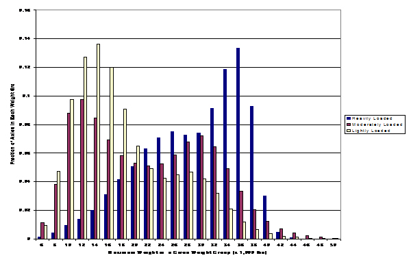
Source: Federal Highway Administration
One important consideration when creating truck weight road groups is whether different road groups will be created for each class of heavy vehicle (meaning a specific road segment can be assigned to nine different groups – one for each class of heavy vehicle), or whether each road segment is assigned to only one group that is primarily formed based on the loads of the most common or voluminous heavy vehicles. The most common approach historically has been to assign each roadway to one and only one truck weight road group. However, the FHWA Long Term Pavement Performance (LTPP) project recently completed a report in 2012, MEPDG Traffic Loading Defaults Derived from LTPP Pooled Fund Study, which grouped WIM sites differently for each class of vehicles. By grouping each set of WIM sites differently for each class of heavy vehicles, the LTPP study team was able to create more standardized groups for each type of vehicle.
Regardless of whether a single road segment is assigned to one or more groups, two key aspects of group formation are:
Finally, it is important to note that for roads with separated right-of-way for different directions of travel, the two different directions of travel can be placed in different groups. For example, the loaded direction might be assigned to a group with a heavy loading pattern, while the other direction of travel (the side carrying primarily empty trucks) might be assigned to a light group. Where the two directions share a single pavement design, the entire road should be assigned to the heavier group for pavement design purposes.
For the LTPP project’s approach of assigning each site to multiple groups (one group per class of vehicle), the development of the groups is performed entirely mathematically. Analysis sites are then assigned to these groups based on professional knowledge. Because the assignment process has considerable error associated with it, users of the LTPP weight groups are strongly encouraged to apply sensitivity tests to their analyses that use these group load spectra (i.e., analysts are encouraged to perform their analyses at least twice, using two different load groups, to test the effects of potential errors caused by improper assignment of the roadway being analyzed to the wrong truck weight load groups).
As with the factor grouping processes described earlier for both vehicle classification and total volume, the basis for the group formation process can be either intuitive or mathematical, or some combination of these two approaches. The intuitive approach is where descriptive information is used along with professional knowledge to create groups of roads that should have similar truck loading patterns due to the nature of the truck traffic they carry. This approach is the easiest to apply but often produces groups that are more variable. The mathematical approaches (most commonly based on cluster analysis) generally create more homogeneous groups, but tend to result in groups that are harder to define, making assignment of roadway sections to groups more difficult. As a result, combination approaches are often tried that start with basic intuitive groups (e.g., geographic stratifications or geographic stratification along with descriptive road classifications such as urban/rural or interstate/non-interstate) and then apply cluster analysis within the initial groups to determine more uniform sub-groups within the basic geographic/roadway classifications.
With this approach, the initial roadway groups used to summarize truck weight characteristics should be based on a combination of known geographic, industrial, agricultural, and commercial patterns, combined with knowledge of the trucking patterns and legal weight limits that occur on specific roads. These initial concepts should then be tested by examining the actual truck weight data collected at WIM sites operated by the State to determine if roads that are expected to have similar loading patterns have similar patterns. The intent is simply to identify those roads that trucks are heavily loaded versus those routes where large numbers of trucks are not carrying very heavy weights.
The resulting road groups for truck weight data should be easily identified by users of truck weight data within the State. They must provide a logical means for discriminating between roads that are likely to have very high load factors and roads that have lower load factors (i.e., between roads where most trucks are fully loaded and roads where a large percentage of trucks are either partially loaded or empty). In addition, States should incorporate knowledge about specific types of very heavy vehicles into their weight grouping process so that roads that carry those heavy trucks are grouped together, and roads that are not likely to carry those trucks are treated separately. For example, roads leading to and from major port facilities might be treated separately from other roads in that same geographic area, simply because of the high load factor that is common to roads leading to/from most port facilities.
In the 1990s, Australia proposed a similar grouping technique in the chapter on traffic data collection in its pavement design guide (Update of the AUSTROADS Pavement Design Guide – Traffic Design Chapter, Final Draft Working Document, September 1998.) In the Australian guide, 25 different truck-loading patterns are identified nationwide. These patterns are structured by type of trucking movement, and the infrastructure linkages being served. The Australian guide uses the following categories of haul activities:
NCHRP Project 1-37A, Development of the 2002 Guide for the Design of New and Rehabilitated Pavement Structures: Phase II developed a similar set of truck weight loading groups from data available in the Strategic Highway Research Program’s Long Term Pavement Performance project Central Traffic Database. The NCHRP project identified 17 different loading conditions and described them with terms similar to the short Australian list noted above.
For a State, it is reasonable to start with less detailed truck weight stratification than these approaches. In fact, unless State data suggests the need for a definitive grouping process, it is recommended that initial intuitive groups be based on a more simplistic approach. For example, insight into geographic differences in truck travel can be used along with the percentage of through-trucks that exist on a road to define roads where loading patterns are dominated by local industry or long haul truck traffic.
Other professional knowledge based criteria that can be used to create truck load groups include:
This simplistic approach would then be improved (as needed) over time as more weight data is collected and analysis carried out. A State may also be interested in discriminating between roads because of the industrial activities they serve. For example, roads leading into and out of major seaports may experience far heavier traffic (higher load factors) than other roads in the same area. Much information can be extracted from existing truck weight databases and planning programs to determine logical and statistical differences that can be accounted for in the formation of truck weight groups.
As an example of a weight factor group, Washington State developed five basic truck-loading patterns as part of a study to determine total freight tonnage carried by all State highways. These five groups were defined as:
A starting point for developing truck weight groups is shown in Table 3-12. The example begins with the groups identified in the vehicle classification section. The truck loading groups defined should be coordinated with the vehicle classification groups identified earlier. Differences in the two sets of groups are likely since the groups are defined to meet different purposes (seasonal differences in truck volume and loading variation). However, they both reflect truck travel characteristics that are directly related. A similar group definition will greatly simplify the understanding and applicability of the patterns. The groups may need further redefinition over time as information is gained.
| Rural | Urban |
|---|---|
| Interstate and arterial major through truck routes | Interstate and arterial major truck routes |
| Other roads (e.g., regional agricultural with little through trucks) | Interstate and other freeways serving primarily local truck traffic |
| Other non-restricted truck routes | Other non-restricted truck routes |
| Other rural roads (mining areas) | Other roads (non-truck routes) |
| Special cases (e.g., recreational, ports) |
These are examples. Each State highway agency should select the appropriate number and definition of truck groups based on its economic and trucking characteristics and the need for heavy vehicle travel patterns in their State.
The 2012 report, MEPDG Traffic Loading Defaults Derived from LTPP Pooled Fund Study, contains very detailed instructions on how to use cluster analysis to group load spectra. This document only summarizes that material.
The cluster process consists of the following steps:
1. Develop a normalized load spectrum from well-calibrated WIM scales for each WIM site.
2. Compute a single statistic for each load spectrum that represents the nature of that spectrum. For example, if the primary reason the group is being created is for pavement design, then convert the normalized load spectrum to some form of estimate of the average damage caused per axle. An ESAL is this type of statistic. One ESAL value should be computed for each normalized load spectrum. If the main use of the truck weight road group is for estimating total tonnage on State routes, then mean axle weight may be used as the best single statistic that represents each normalized load spectrum.
3. If the load spectra for all heavy vehicle classes at a WIM site are to be assigned to only one truck weight road group, determine how different loading patterns for each class of vehicle will be weighed. (This step is not necessary if groups will be formed for each type of axle for each class of vehicle.)
4. Perform a cluster analysis, stopping when clusters reach the point where the difference between clusters becomes large enough that the use of different clusters causes statistically different outcomes when used in planned analyses.
Steps 3 and 4 are discussed in more detail below. Step 1 requires no additional explanation. Step 2 has been demonstrated already in Table 3-11 above
Step 3 determines how to handle grouping because different classes of trucks will have different patterns at any given site. That is, some classes of trucks will be heavier at one site (Site A) than at other sites (e.g., Sites B through G), while a different set of vehicle classes will be lighter at Site A than at the remaining sites. Finally, other vehicle classes will have very similar patterns. The difficult task in grouping these sites is determining how to weigh the relative importance of these different vehicle classification weight patterns.
For example, at Site A, the Class 9 truck weight pattern may be dominated by urban delivery trucking patterns where Class 9 trucks are equally split between load, unloaded, and partially loaded conditions. At the same site, Class 7 and Class 10 vehicles may all be carrying very heavy loads. At Site B, the majority of Class 9 trucks are fully loaded, while Class 7 and Class 10 are also carrying heavy loads. At Site C, the original Class 9 urban pattern is present, but the Class 7 and 10 vehicles are much lighter than elsewhere. In step 3, it is necessary to determine if these three sites should be grouped together or kept separately. (If groups are formed differently for each class of vehicles, Sites A and C would be grouped together for Class 9 trucks with Site B kept as a different group, but Sites A and B would be grouped together for Classes 7 and 10, with Site C separate this time.) If only one group can be formed, Step 3 should be used to determine which of these patterns is most important to the formation of the group.
If all vehicle classes are treated equally, a statistically based cluster analysis might group all three of these test sites or it might separate all three sites, depending on the criteria set when applying the clustering approach. However, not all trucks are equal. Some truck classes are heavier than others (Class 5 is considered a truck, but is generally so light it creates little pavement damage, while Classes 7 and 10 tend to always be heavy and can be extremely heavy.) Similarly, while some trucks are very heavy, there are often less of them compared to other moderately heavy trucks. Thus, while trucks in Classes 7 and 10 tend to be very heavy, in most States and on most roads, these classes are a very small percentage of truck traffic, and contribute a relatively modest amount of total pavement damage. On some roads, these trucks are very prevalent and drive the pavement design equation. In most cases, however, Class 9 tends to produce the vast majority of pavement loading from traffic. These trucks tend to be less damaging per vehicle, but they tend to constitute a very large percentage of truck volumes. Therefore, when deciding how to balance the importance of different truck classes to the grouping process, a combination of how heavy each class is and how frequently they are observed are important considerations.
While considerably more research is needed on the best methods for grouping truck-loading patterns, the recommendation in this report is to identify the one or two most significant truck patterns. This can be computed by multiplying the volume of that class of trucks times their average weight. Any truck class that provides more than 40 percent of the total load on a pavement should be considered in the grouping process.
This simplifies the grouping process, although it downplays the importance of lower volume truck classes in that process. States can always refine their grouping process to better account for lower volume classes as they refine their traffic-monitoring program.
In Step 4, the data that represents the vehicle class loading conditions being used to group sites are entered into a statistical clustering program. The output of that process can then be tested to determine the reliability of the groups created. (See subsection, “Testing the Quality of Selected Truck Weight Groups” on page 3-51.)
The last approach described in this report combines features of the Intuitive and Clustering Approaches. In this approach, professional judgment is used to initially segregate roads into specific categories or groups. For example, based on data from classification counts, the State may know that specific roads carry large volumes of Class 7 and Class 10 trucks due to the nature of industry served by those roads (e.g., coal or other heavy natural resources.) These roads may be segregated from roads that carry more diverse heavy vehicle traffic prior to running cluster analyses. These roads may be used as one group, or a cluster analysis may be performed using only data from WIM sites on these special roads – using Class 7 and Class 10 loading conditions as the key cluster variable. A separate cluster analysis may then be applied – using Class 9 loading conditions as the cluster variable – for all other roads in the State.
This hybrid approach to truck weight road group creation is intended to improve the group creation process by allowing application of professional knowledge in limited ways, while preserving the statistical integrity of the group creation as much as possible with the clustering approach whenever current knowledge does not provide clear definition of truck load groups.
Just as with the formation of groups used for factoring volume and classification counts, the initial formation of heavy vehicle weight groups should be reviewed to determine whether the road segments grouped together have similar truck weight characteristics. Examining available data from the existing truck weight sites is the first step. A substantial amount of judgment is required since the data is likely to be limited to that currently available from existing WIM sites.
For example, a State highway agency may find that in one group of roads, the Class 9 trucks all have similar characteristics, but the Class 11 truck characteristics are very different from each other. By changing the road groups, it may be possible to classify roads so that all Class 9 and Class 11 trucks within a road group have similar characteristics. More likely it will not be possible to form homogenous groups for different truck classes, and trade-offs will have to be made. The type of vehicle considered the most important should be given priority.
The trade-offs can be made based on the relative importance of each weight statistic to the data user. In many cases, this is simply a function of determining the relative importance of different truck statistics. For example, if 95 percent of all trucks are in Class 9, then having truck weight road groups that accurately describe Class 9 truck weight characteristics may be more important than having road groups that accurately describe Class 11.
An estimate of the precision of the mean of a variable that any truck weight road group will provide can be found by computing the standard deviation when computing the mean statistic for that variable. For example, the precision of the mean gross vehicle weight for a Class 9 truck within a truck weight group can be calculated while computing the mean GVW per Class 9 truck from all of the WIM sites within that group. The standard deviation of the estimate and the number of sites provide an approximate measure of the precision of the mean of the group.
An example of this computation is shown below. In the example, assume that a State has determined that all rural interstate roads have similar truck weight characteristics based on seven WIM sites. Statistics from those WIM sites are shown in Table 3-13. Based on this data, it can be assumed that all rural interstate roads in the group have a mean gross vehicle weight of 25,000 kg for Class 9 trucks. To determine an estimate of precision of this group with respect to pavement design, the mean ESAL value for flexible pavements is also computed for these sites in Table 3-13. As can be seen, the average Class 9 truck in this group of sites applies an average of 1.63 ESAL. (When comparing ESAL values between sites, the ESAL computations assume the same pavement type and structure. All ESAL examples in this document are computed assuming flexible pavements. ESALs are used in this chapter as the measure of pavement damage because they are still in common use in most States. While they have limitations as a measure of traffic loading for pavement design, and are being phased out of many pavement performance analyses, they are still a very useful single statistic for comparing the load spectrum in terms of the amount of pavement damage that those load spectrum will cause. Other summary statistics can be used in place of ESALs to simplify the comparison between load spectrum.)
The precision of the group mean, referred to as the standard error of the mean, can be estimated with 95 percent confidence as approximately plus or minus 1.96 times the standard deviation divided by the square root of the number of sites. (This is a relatively crude approximation. The value 1.96 should be used only for sample sizes of 30 sites or more. A more statistically correct estimate would use the student’s t distribution, which for six degrees of freedom (seven weigh sites) is roughly 2.45.)
| Site | Mean Class 9 GVW |
Mean Class 9 ESAL |
|---|---|---|
| 1 | 50,000 lb |
1.64 |
| 2 | 57,000 lb |
1.72 |
| 3 | 64,000 lb |
1.84 |
| 4 | 46,000 lb |
1.45 |
| 5 | 45,000 lb |
1.34 |
| 6 | 55,000 lb |
1.65 |
| 7 | 62,000 lb |
1.78 |
| Group Mean | 54,000 lb |
1.63 |
| Group Standard Deviation | 7,500 lb |
0.18 |
| Coefficient of Variation | 0.14 |
0.11 |
| Standard Errors of Mean | 2,800 lb |
0.07 |
In the above example, note that the coefficient of variation for the two statistics (GVW/vehicle and ESAL/vehicle) are different, even though both variables come from the same set of vehicle weights. Each statistic computed for a truck weight group is likely to have different statistical reliability because of the different levels of variation found in axle weights, GVW, and the various other statistics computed from weight records
To complicate matters further, each statistic has a different level of precision for each different vehicle class. Accordingly, the precision of the ESAL/vehicle value for Class 9 trucks will be different from that of the ESAL/vehicle value for Class 11 trucks.
The precision calculations can be used to determine how many WIM systems should be included within each truck weight group. The State highway agency should determine what statistic it wants to use as the key to the analysis, select how precisely it wishes to estimate that statistic, and compute the number of WIM locations needed to obtain the desired degree of confidence.
This step involves several decisions
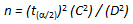
Where:
n = the number of samples taken (in this case, the number of sites in the group)
t = the student’s t distribution for the selected level of confidence (α) and appropriate degrees of freedom (one less than the number of samples, n)
α = the selected level of confidence
C = the coefficient of variation (COV) for the sample as a proportion
D = the desired accuracy as a proportion of the estimate
Table 3-14 shows the same truck weight statistics used in Table 3-13, except two additional weight sites have been added. These two sites experience heavy vehicle weights and consequently have increased the mean values for GVW/vehicle and ESAL/vehicle for the group.
| Site | Mean Class 9 GVW |
Mean Class 9 ESAL |
|---|---|---|
| 1 | 50,000 lb |
1.64 |
| 2 | 57,000 lb |
1.72 |
| 3 | 64,000 lb |
1.84 |
| 4 | 46,000 lb |
1.45 |
| 5 | 45,000 lb |
1.34 |
| 6 | 55,000 lb |
1.65 |
| 7 | 62,000 lb |
1.78 |
| 8 | 77,000 lb |
2.01 |
| 9 | 75,000 lb |
1.95 |
| Group Mean | 59,000 lb |
1.71 |
| Group Standard Deviation | 11,600 lb |
0.22 |
| Coefficient of Variation | 0.197 |
0.13 |
| Standard Error of Mean | 3,900 lbs |
0.07 |
Using this table the following can be determined
Increasing the number of WIM stations included in the sample to 15 sites (and assuming that those stations do not change the standard deviation of the sample) would change the standard error of the mean to 3,000 kg (11,600 divided by the square root of 15). This would improve the confidence in the mean value of the GVW/vehicle estimate for the truck weight group to 59,000 lb +/- 6,400 lb with 95 percent confidence. The improvement comes from two sources. The first is the increased precision in the mean value provided by the increase in the number of samples. The second is the decrease in the value of ta/2 used to compute the multiplier in the confidence interval by having a greater sample size upon which to perform the statistical computation.
Table 3-15 shows the effect of different sample sizes and confidence intervals estimates of the group mean. Note that increases beyond about six sites in the group sample size have only a marginal effect on the precision of the group mean
| Number of Weigh Sites[1] |
Mean Value |
Precision of the Mean Value Itself(Standard Error |
|
|---|---|---|---|
Precision of the Mean Value Itself(Standard Error |
Precision of the Mean Value Itself(Standard Error |
||
| 3 | 59,000 lb |
12,600 lb |
28,800 lb |
| 5 | 59,000 lb |
8,000 lb |
14,400 lb |
| 9 | 59,000 lb |
5,400 lb |
8,900 lb |
| 15 | 59,000 lb |
4,000 lb |
6,400 lb |
| 30 | 59,000 lb |
2,700 lb |
4,200 lb |
| 60 | 59,000 lb |
1,900 lb |
2,900 lb |
| 90 | 59,000 lb |
1,600 lb |
2,400 lb |
This table uses the student’s t distribution because of the small number of sample sites in the group.
The value of tα/2 for each sample size using the student’s t distribution for a two-tailed confidence interval of α = 80% (t.1) is as follows: n = 3, tα/2 = 1.886, n = 5, tα/2 = 1.533, n = 9, tα/2 = 1.397, n = 15, tα/2 = 1.345, n = 30, tα/2 = 1.282.
The value of tα/2 using the student’s t distribution for a two-tailed confidence interval of α = 95% (t.025) is: n= 3, tα/2 = 4.303, n= 5, tα/2 = 2.776, n= 9, tα/2 = 2.306, n= 15, tα/2 = 2.145, n= 30, tα/2 = 1.960.
If tighter confidence intervals are deemed necessary, it is always possible to modify the truck weight road groups. Looking at Table 3-14, it is apparent that sites eight and nine have much higher loads than the remaining seven sites. If these sites are removed from the truck weight group, the computed standard deviation of the GVW per vehicle computed for sites in the group drops from 11,600 lb to 7,500 lb. This has a dramatic impact on the precision of the estimates computed for the group.
Table 3-16 shows the precision level of the truck weight group after removal of these sites. However, note that to remove these two sites from the truck weight road group, they should represent some identifiable set of roads. For example, they could be located on the State’s only north/south rural interstate, while the remaining seven sites are on east/west interstates. Therefore, the rural interstate truck weight grouping could be divided into two separate truck weight groupings, rural east/west interstate and rural north/south interstate.
| Number of Weigh Sites[1] |
Mean Value |
Precision of the Mean Value Itself(Standard Error ) |
|
|---|---|---|---|
80% Level of Confidence[2] |
95% Level of Confidence[3] |
||
| 3 | 54,000 lb |
+8200 lb |
+18600 lb |
| 5 | 54,000 lb |
+5100 lb |
+9300 lb |
| 9 | 54,000 lb |
+3500 lb |
+5800 lb |
| 15 | 54,000 lb |
+2600 lb |
+4200 lb |
| 30 | 54,000 lb |
+1800 lb |
+2700 lb |
| 60 | 54,000 lb |
+1200 lb |
+1900 lb |
| 90 | 54,000 lb |
+1000 lb |
+1600 lb |
This table uses the student’s t distribution because of the small number of sample sites within the truck weight road group.
The value of tα/2 for each sample size using the student’s t distribution for a two-tailed confidence interval of α = 80% (t.1) is as follows: n = 3, tα/2 = 1.886, n = 5, tα/2 = 1.533, n = 9, tα/2 = 1.397, n = 15, tα/2 = 1.345, n = 30, tα/2 = 1.282
The value of tα/2 for each sample size using the student’s t distribution for a two-tailed confidence interval of α = 95% (t.025) is as follows: n = 3, tα/2 = 4.303, n = 5, tα/2 = 2.776, n = 9, tα/2 = 2.306, n = 15, tα/2 = 2.145, n = 30, tα/2 = 1.960
The key to correctly creating these truck weight groups is that sites should only be removed from a truck weight group when they can be readily identified with a specific set of roads that experience those loads. All of those roads should be moved to the new truck weight group.
From the above examples, it is possible to see that changing the number of sites included in a truck weight road group has three effects:
1. It changes the computed sample standard deviation for the group (which serves as the estimate of the standard deviation for the entire road group).
2. It changes the denominator used to compute the standard error, which is the statistic used to determine how well the mean value computed from that group of roads estimates the mean value for the population being sampled.
3. It changes the value of t used to compute the size of the confidence interval applied to estimates produced for that group.
In general, the more sites included in a group, the better the estimates produced by that group, although the benefit of adding sites decreases as the number of sites within a group increases. The effect of using the student’s t distribution to compute confidence intervals means that a significant decrease in the value of t can be obtained by simply adding locations up to a sample size of six. A sample size of six sites has a 10 percent smaller confidence interval at the 95 percent level of confidence than a sample size of five sites, all other things being equal. Beyond six sites, the benefits gained by adding sites begin to decrease quickly. More than six sites in a group may be appropriate, particularly if the State is unsure of its truck weight patterns.
Based on this analysis, six sites per group are recommended. The exception to the six-site rule is for truck weight road groups that contain very few roads. These will tend to be specialty roads (e.g., roads leading into and out of gravel pits) that have unusual loading conditions but that are not applicable to many other roads in the State. If improvements in precision are needed beyond what affordable increases in sample size will achieve, the primary option is to change the make-up of the truck weight groups, i.e., create new subsets of roads that will serve as the truck weight groups. If this change produces a significant decrease in the standard deviation that offsets the increase in tα/2 caused by the lower sample size, then the State will benefit from an improvement in the precision of its weight estimates along with a smaller data collection sample size.
All of the statistics presented previously start with the critical assumption that each WIM site in a truck weight group produces an accurate estimate of vehicle weights for that location, so that the mean value calculated for the group is accurate. The accuracy assumed for the data provided by each WIM scale is not just that the scale weighs the passing trucks correctly, but that those weight estimates are representative of weights at that site throughout the year.
For WIM sites where less than a year of data is collected, the assumption is that the period measured gives an accurate measurement of weights for the entire year. If the weight data collection period is only 48 to 72 hours, the assumption is that there is no DOW difference in the loading condition of trucks passing the site. That is, that trucks traveling on weekends carry the same distribution of payloads as trucks traveling on weekdays, as well as the hypothesis that there are no seasonal differences in truck loading patterns. At some WIM sites in some States, extensive data collection has shown that these assumptions are reasonable (Butler 1993). At other sites and in other States, these assumptions are incorrect (Hallenbeck and Kim, 1993). Where truck weights are not stable across days of the week or seasons, the weight monitoring effort has to be extended to account for these differences. For example, the count duration may be extended from two days to seven days to incorporate DOW differences. Seasonal differences can be detected and incorporated in the annual estimates by collecting data at each site more than once per year, such as once per quarter.
While it is mathematically possible to obtain load spectra information through factoring of short duration WIM data to account for variations in seasonal changes in truck loading patterns, this process is not recommended due to the limited data available to create and apply those adjustments. Where seasonal differences in load spectra are known or suspected (for example, seasonal load restrictions occur in that area), States are encouraged to collect sufficient data to measure those changes rather than trying to factor short duration WIM measurements to estimate those changing patterns. If a State chooses to factor the load spectra information from short duration WIM for pavement design purpose, formal consultation should be carried out with the Federal Highway Administration.
To date, little work has been published on the seasonal differences in axle weight distributions found in the nation’s truck fleet, nor on the weight characteristics of particular trucking movements found in individual States. However, these seasonal and DOW weight changes can have dramatic effects on the selection of the pavement designs that rely on them. The collection and analysis of continuous data collection is the easiest method to begin to understand the temporal variation.
The key for the weight data collection program is to measure and account for both DOW and seasonal differences in vehicle weights within each truck weight group. The only way to do this adequately is to have each WIM station providing continuous WIM data, unless analysis has shown that temporal variability is not present. For States with large numbers of continuous WIM stations, sufficient stations to populate the groups likely already exist. For smaller States facing resource limitations, the installation of many continuous WIM sites is not as feasible. The general recommendation is that each truck weight group should have at least one, and preferably more than one, continuous WIM device collecting continuous data. This site should be maintained in a calibrated condition, and the data obtained from it should be used to determine whether significant differences exist between vehicle weights (by vehicle class) for different days of the week, months of the year, and year to year. Where resources are limited and neighboring States have similar truck size and weight laws, States can share WIM data to create weight groups where site groups can come from more than one
The remaining sites within a group can have either short duration counts or additional continuous counts. As with vehicle classification and volume counting, a minimum of 48 hours should be used. Weight data has been shown to vary by time of day, day of week, weekdays, and weekends. As with vehicle classification and volume counts, it is acceptable to use different data collection periods as needs and constraints allow. Because of differences in weekday and weekend vehicle weights, the data collection program should be designed to cover those differences and account for them when statistics are produced. Counts taken for a period of one week eliminate the need for DOW adjustment, allow the equipment and traffic conditions to stabilize, provide data verification capabilities, and identify weekday/weekend differences in average weights. A monitoring period of seven continuous days is recommended for all WIM sites that do not provide continuous data.
Short duration WIM measurements should be collected with permanently mounted sensors because permanent sensors can be mounted flush to the road surface, providing a more accurate weight measurement. (Permanent sensors include sites where the sensors are permanently installed but only used periodically; sites where the sensors are installed permanently but the electronics removed from the roadside when not in use, and sites where semi-permanent sensor frames are permanently installed but the actual sensors are replaced with a dummy scale when not in use.) Use of permanently mounted sensors also allows data collection periods to be lengthened at relatively little additional cost.
Portable sensors introduce accuracy issues that may compromise the validity of the data, although they are not completely ruled out. Organizations using portable WIM sensors should carefully ensure that the data collected is sufficiently accurate to meet user needs.
Many issues are to be considered when installing WIM sites. Current installations range from full coverage for all lanes and directions of travel to the LTPP standard of a single lane in one direction. Some of the issues to be reviewed when selecting the number of lanes of WIM to install include:
Analyses of available WIM data have shown that significant differences in loads by direction of travel often occur. The collection of WIM data in at least one lane in each direction of travel at each site allows a clear assessment of directional differences in weights and loadings. WIM differences by travel lane are generally less significant and difficult to generalize, although previous analyses have shown that the outside lanes tend to carry heavier vehicles. More analysis of current installations is needed before a determination of the cost-effectiveness of covering several lanes at some of the WIM sites or at all sites can be made.
A WIM site covering all lanes and direction of travel provides the most complete data collection coverage. At least one continuous WIM station in each weight group should provide WIM coverage for all or a minimum of two travel lanes in each direction. This will allow future pavement design analysis to cover most possibilities. For multi-lane facilities, covering two lanes in each direction provides the most cost-effective alternative. If some lanes are not monitored by WIM sensors, each WIM site should have, at a minimum, a portable classification count by direction and travel lane to measure truck travel in the lanes not being monitored with WIM. Continuous classification in those lanes is preferable. Figure 3-12 shows examples of this.
A. Best: WIM Covers All Lanes and Directions
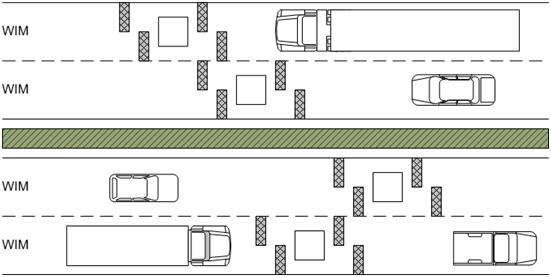
B. Better: WIM or Two Permanent Axle Sensors in All Lanes
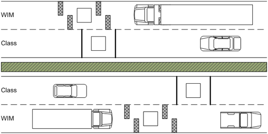
C. Good: Two Portable Axle Sensors in All Lanes
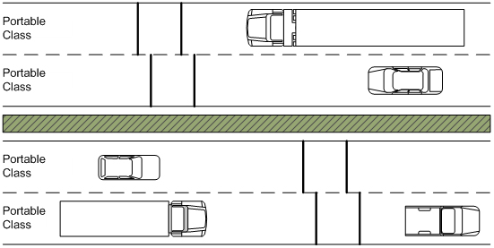
Source: Federal Highway Administration.
WIM systems also provide counts of vehicle volume by classification, speed, and total volume. Consequently, WIM data collection locations can also provide volume and vehicle classification count data that can take the place of counts required to meet the needs reviewed in sub-sections 3.2.1 and 3.2.2. Unfortunately, for a variety of technical reasons, WIM data cannot be collected on all roadway sections. Physical constraints on many road sections prevent the collection of accurate weight data. In addition, most States do not have the resources to collect weight data at more than a modest number of locations. Finally, most States already have a significant investment in WIM sites, either as part of their existing truck weight-monitoring program or as part of the LTPP.
Each State should begin to apply the procedures assessed with its existing WIM data collection sites. Because of the study, the addition of sites may become necessary. As existing sites require attention because of failure of the pavement surrounding the WIM sensors or failure of the WIM equipment itself, the need for that WIM station or site should be reevaluated. Sites that are still needed should be reinstalled. If that site is no longer needed or if other higher priority locations exist, the WIM equipment should be moved to another site.
The selection of new WIM sites should be based on the needs of the data collection program and the site characteristics of the roadway sections that meet those needs. The needs of the data collection program include, but are not limited to, the following:
However, just because a roadway section meets some or all of the above characteristics does not make it a good WIM site. With current technologies, WIM systems only accurately weigh trucks when the equipment is located in a physical environment that meets specific criteria. Therefore, States should place WIM equipment only in pavements that allow for accurate vehicle weighing. While individual equipment vendors may require slightly different pavement characteristics to achieve specified results, in general all WIM sites should have the following (An excellent reference for learning about WIM site requirements is ASTM Standard E-1318, Highway Weigh-in-Motion (WIM) Systems with User Requirements and Test Method. Another excellent source is States’ Successful Practices Weigh-in-Motion Handbook):
In addition, there should be sufficient truck traffic at the site to justify the installation of a WIM data collection site. The actual sites can be selected randomly or judgmentally (using the previous list of criteria) from sites that meet all of the site requirements. Smooth, strong pavement is needed to reduce the effect of vehicle dynamics. Although placing multiple sensors in series (Cebon 1999) can significantly reduce the error that vehicle dynamics produce in individual weight measurements, placement of WIM sensors on smooth, flat pavements that reduce vehicle dynamics significantly improves WIM accuracy, regardless of the equipment used.
Pavement strength can affect sensor accuracy. Weight estimates produced by strip sensors (such as piezo-cables) that are embedded directly into pavements are often affected by changes in pavement strength caused by changes in environmental conditions (e.g., AC flexibility for spring thaw periods). A decrease in pavement strength invariably decreases system accuracy. Therefore, WIM sensors should only be placed in strong pavements that are not subject to significant changes in structural response during different seasons. Similarly, WIM sensors begin to become inaccurate as soon as pavements start to rut. In most cases, installations in pavements likely to rut are a poor investment of limited data collection funds.
The requirement for constant vehicle speed (which limits the use of WIM equipment in many urban and suburban areas where routine congestion occurs) is primarily because braking and acceleration causes shifts in load from one set of axles to another. This shifting causes inaccurate comparison of WIM estimates against static loads.
The availability of power and communications allows extended operation of the WIM equipment. While this is not as crucial for sites intended for short duration WIM counts, the availability of power allows the collection of longer duration or continuous WIM measurements. This is particularly helpful for research studies intended to confirm or refute the ability of short duration counts to meet the accuracy needs of the data collection plan. It also allows the WIM site to be used as a continuous classifier or continuous counter even while weight data is not being collected.
Even with all of the constraints described above, most of the existing sites can be used to meet a given need. When exploring alternative sites, the ultimate decision can often be made by examining how well these alternative sites fit within the existing State traffic monitoring program.
Sites selected for WIM data collection should be located within HPMS volume sample sections, if possible. If two alternative sites exist to meet a specific need and one is already an HPMS sample site, it should be given priority over the alternative (all other factors being equal). If neither site falls on an HPMS sample section, the selected WIM site should become an HPMS sample section the next time the HPMS sample is revised. The HPMS volume and classification data should be collected at the same time as the WIM data, using the same equipment where practical. This reduces the staffing and resources needed to collect these HPMS data and directly ties the different data items.
The recommendations evaluated above lead to the conclusion that the size of the weight data collection program will be a function of the variability of the truck weights, accuracy, and precision desired to monitor and report on those weights.
For a small State that has only two basic truck weight road groups, the basic recommendation is to have a minimum of approximately 12 weighing locations with a minimum of four continuously operating weigh-in-motion sites. The number of locations could be further reduced if the State worked with surrounding States to collect joint vehicle weight data. A larger State with diverse trucking characteristics might have as many as 10 or 15 distinct truck weight road groups, and accordingly 60 to 90 WIM sites, with a corresponding increase in the number of continuously operating WIM locations. Most States will be between the two extremes presented, and the number of weighing locations should fall somewhere between 12 and 90 locations.
Many continuous traffic monitoring devices can produce traffic performance statistics, in addition to those described above, that can be used for other important analytical tasks. In some cases, these statistics should be routinely collected, stored, and reported as part of the traffic monitoring program. In other cases, the added data collection capability should be simply noted and used only when required for a special study.
For example, inductive loop detectors and other devices that mimic loop output, such as video image-based counters, can produce lane occupancy statistics that describe the percentage of time that a vehicle occupies the detection zone. This value can be converted into a reasonable measure of vehicle density. Lane occupancy can also be used as a direct measure of congestion. Many urban freeway and arterial performance monitoring programs use lane occupancy measurements to describe the onset and duration of congested conditions. For example, the Washington State Department of Transportation uses lane occupancy values above 35 percent to indicate the formation of stop-and-go congestion.
Traffic monitoring devices that time stamp the passage of either individual vehicles or the axles of individual vehicles can be used to report the headway between vehicles and/or the time gap between vehicles. These statistics are useful for a number of specific operational analyses but are not routinely reported as an output of most traffic monitoring programs. Consequently, most headway and gap information is collected and reported as part of special studies. However, some traffic monitoring systems—such as weigh-in-motion scales—routinely collect time-stamped vehicle records that can be used to estimate vehicle gap and headways. When States collect data using the new PV format, occupancy, headway, and gap can all be a by-product.
Short duration traffic volume counts are traditionally the primary focus of most statewide traffic monitoring efforts. They provide the majority of the geographic (spatial) diversity needed to provide traffic volume information on the State roadway system.
The recommended short duration volume-counting program is divided into coverage count and special needs count primary subsets. The coverage count subset covers the roadway system on a periodic basis to meet both point-specific and area needs, including the HPMS reporting requirements. The special needs subset comprises additional counts necessary to meet the needs of other users. This second category of counts can be further subdivided into counts taken to meet State-specific statistical monitoring goals, to provide increased geographic coverage of the roadway system, and to meet the needs of specific project or data collection efforts. Each of these categories of counts is presented in the following paragraphs.
Short duration counts ensure that adequate geographic coverage exists for all roads under the jurisdiction of the highway authority. In simple terms, coverage counts are data collection efforts that are undertaken to ensure that at least some data exist for all roads maintained by the agency. How much data should be collected to provide adequate geographic coverage is a function of each agency’s policy perspective. Some State highway agencies consider a weeklong count every seven years with data recorded for every hour of each day to be adequate. Others consider a 48-hour count every 3 years with no hourly records to be adequate. Clearly, significant utility can be gained from having at least hourly volume estimates at coverage counts, since that data can be used to obtain a much more accurate understanding of traffic volume peaks during the day. As indicated in Section 3.2.3, at a minimum the TMG recommends that State highway agencies initially aim to collect 25 to 30 percent of their short-duration counts with classification counting equipment. Agencies that can exceed this figure are encouraged to do so. The ability to meet or exceed this goal depends on agency perspective and is a function of the equipment available and the nature of the road system.
The following steps apply to short classification counts:
1. Divide the road system into homogeneous traffic volume segments; determine the count locations needed to cover the system over a maximum cycle of six years.
2. Determine the count locations required to meet the HPMS and other data needs by reviewing HPMS manuals.
3. Determine the count locations and data collection needs of specific projects that will require data in the next year or two. This entails working with the offices that will request this data to determine their data needs. This coordination should occur on a continuous basis to ensure counts for special projects are collected when needed.
4. Overlay the counts on maps of the highway system including the location of functioning continuous counters.
5. Determine how counts can be combined to make best use of available counting resources.
6. Schedule the counts to use the available data collection crews and equipment efficiently.
These steps are intended to reduce count duplication and increase the efficiency of the data collection staff.
The spacing between short duration counts in a roadway is also subject to agency discretion. This method for section length should also be detailed in the State TMS plan. The primary objective is to count enough locations on a roadway so that the traffic volume estimate available for a given highway segment accurately portrays the traffic volume on that segment. Generally, roadway segments are treated as homogenous traffic sections (that is, traffic volumes are the same for the entire segment). For a limited access highway, this is true between interchanges. However, it is also true for all practical engineering purposes for a rural road where access and egress along a ten-mile segment is limited to a few driveways and low volume, local access roads. Highway agencies are encouraged to examine existing traffic volume information to determine how best to segment their roadway systems to optimize the number and spacing of short duration counts. A rule of thumb that has been used in the past to define these traffic count segments is that traffic volume in each roadway segment be within 10 percent. An alternative approach would be to define limits using a graduated scale such as the one shown in Table 3-17.
| Beginning Segment AADT | Adjoining Segment AADT Within |
|---|---|
| 100,000 or more | + 10% |
| 50,000 – 99,999 | + 20% |
| 10,000 – 49,999 | + 30% |
| 5,000 – 9,999 | + 40% |
| 1,000 – 4,999 | + 50% |
| Less than 1,000 | + 100% |
Breaking the system into very large segments reduces the number of counts needed but also the reliability of the resulting traffic estimates for any given section of that large roadway segment. Use of small segments increases the reliability of a specific count but also the number of traffic counts needed.
The character of the road systems and the volumes carried has a major impact in the definition of segments. For roads where access is controlled (such as the interstate system), a simple definition of segments between interchanges is appropriate. For lower systems, clear traffic volume breaks are not always apparent and other rules of thumb (such as major intersections) should be applied. Rural and urban characteristics also require different handling. For the lowest volume roads, the 10 percent rule of thumb may be too narrow and a wider definition sought. Careful definition of roadway segments can significantly reduce the number of counts needed to cover all highways within an agency’s jurisdiction, while still providing the accurate volume data required for planning and engineering purposes.
Once roadway segments are finalized, the FHWA recommends as a rule that each roadway segment be counted at least once every six years. This ensures that reasonable traffic volume data is available for State needs, and that all roadway segments are correctly classified within the proper HPMS volume groups when State highway agencies compute statewide VDT as part of their required Federal reporting. HPMS further requires counting every three years for higher functional class roadways.
Not all count locations should be counted on a six-year basis. Some count locations should be counted more often. Other roads can be counted less frequently without loss of volume estimate accuracy. In general, roadway sections that experience high rates of growth require more frequent data collection than those that do not experience growth. Therefore, roads near growing urban centers and expanding recreational sites should be counted more frequently than roads in areas where activity levels have hardly changed for many years. Counting roads more frequently in volatile areas also allows the highway agency to respond with confidence to questions from the public about road use (a common concern in high growth areas), and ensures that up-to-date by lane and directional statistics are available for the roadway design, maintenance, and repair work that is common in high growth areas.
The short duration count data collection program itself can be structured in many ways. One simplistic approach is to randomly separate all of the roadway segments into unique sets and count one of these sets each year. However, this approach does not always lend itself to efficient use of data collection staff and equipment. Grouping counts geographically leads to more efficient data collection activity, but results in the need to account for the geographic bias in the data collected when computing annual average traffic statistics or looking at trends in traffic growth around the State.
In addition, most highway agencies collect data at some sites on a cycle shorter than six years. For example, more frequent counts (three-year cycle) are required on HPMS sections, and most States count higher system roads more frequently as well. Still, considerable flexibility is allowed in the structure of each agency’s short duration count program.
The HPMS standard sample meets the need for computation of a statistically reliable measure of statewide travel. The data collected also cover many highway agency needs. However, there remain traffic data needs that cannot be met by the short duration count program. This is where an effective short duration program supplemented by special counts can substantially fill the gap.
Non-HPMS data needs vary dramatically from State to State and from agency to agency. Some State highway agencies are responsible for almost all road mileage in their State. Other State highway agencies control, operate, and maintain only the largest, most inter-regional facilities. Some States must meet strict reporting requirements (by jurisdiction) adopted by their legislatures. Others have relatively few mandatory reporting requirements, and instead focus on collecting data that meet each particular agency’s priorities. In some extreme cases, agencies are prohibited by law from expending resources outside of their areas of responsibility.
A consequence of this variety of traffic data needs is that no single traffic monitoring program design fits all cases. Therefore, the philosophy of the special needs element is to provide highway agencies wide flexibility to design this portion of their monitoring program in accordance with their own self-defined needs and priorities. The guidance in this report is intended to provide highway agencies with a framework within which they can ensure that they collect the data they need.
The special needs portion of a data collection program can be divided into two basic portions:
Statistical samples such as the HPMS are the most efficient way to estimate population means and totals. Most statistical samples involve the collection of data at randomly selected locations to compute unbiased estimates of population means and totals. Random sampling is a very efficient mechanism for computing these totals.
A variety of texts is available on the design of samples. Sampling Techniques is one such standard text. The HPMS Field Manual provides a description of how the HPMS sample was developed and implemented. These documents are useful in helping design a sampling program to meet objective needs. The keys to successfully designing a statistical sampling plan are defining the objectives, understanding the variability of the data being sampled, having a clear understanding of what statistics should be computed, and establishing the accuracy and precision of the estimates. Any statistical samples developed should make use of the available data from the short duration element to minimize the duplication of effort, as much as possible. One possible use of statistical samples is to estimate VMT for the local functional systems, where extensive mileage makes the collection of traffic data very costly.
Unfortunately, the random selection of count locations required by most statistical samples is an inefficient mechanism for meeting many site-specific traffic data needs. For example, an uncounted roadway section is not a major concern for HPMS because the sample expansion process represents all road sections in the statewide VMT estimation. However, if pavement needs to be designed for that section of roadway, a statewide average or total is not a substitute for one or many traffic counts specific to that road section.
Consequently, data needs require agencies to collect data at locations that are not part of the short duration program. However, by maximizing the use of available data, it is possible to keep the number of these special counts to a minimum and to save resources for other data collection and analysis tasks. No additional data should be collected if existing data meet the desired need.
Special counts are generally required for specific project needs. Project counts are undertaken to meet the needs of a given study (for example, a pavement/corridor study, rehabilitation design, or a specific research project). These cover a range of data collection subjects and are usually paid for by project funds. Project counts are traditionally taken on relatively short notice, and they often collect data at a greater level of detail than for the short duration or the HPMS parts of the program. Often, the need is not realized until after a project has been selected for construction, and insufficient time exists by that date to schedule the project counts within the regular counting program. However, where it is possible to include project counts within the regular count program’s schedule, significant improvements in staff utilization and decreases in overall costs can be achieved.
Many different types of counts can fall within the special needs element. Counts are taken by many public and private organizations for many purposes including intersection studies, signal warrants, turning movements, safety analysis, and environmental studies. As much as possible, these activities should be coordinated within the program umbrella.
In general, roadway sections that experience high rates of growth and recreational areas require more frequent counting than those that do not experience growth. Counting roads frequently in volatile areas allows the highway agency to respond with confidence to questions from the public about road use (a common concern in high growth areas), while also ensuring that up-to-date statistics are available for the roadway design, maintenance, and repair work that is common in high growth areas. Many agencies prefer the use of several counts a year to understand the traffic variability inherent in high growth better. Likewise, recreational roads usually experience major traffic peaking at specific times necessitating frequent data collection times.
High growth areas (if not necessarily roads with high volume growth) can usually be selected on the basis of knowledge of the highway system and available information on the construction of new travel generators, highway construction projects, requirements for highway maintenance, applications for building permits, and changes in population. Recreational areas are also well known to experienced transportation professionals.
Cost efficiency in the traffic-monitoring program is best achieved by carefully coordinating the different aspects within the program. This includes both continuous and short duration counts. It also includes the short duration, HPMS, and special needs counts
In theory, the highway agency would start each year with a clear understanding of all of the counts that need to be performed. The list could then be examined to determine whether one count could be used for more than one purpose. For example, a classification count at one interstate milepost might easily provide the data required for both that count and a volume count required at the next milepost, since no major interchanges exist between those mileposts. By careful analysis of traffic count segments, location, and data requirements, it is often possible to significantly reduce the total number of counts required to meet user needs.
The next step is to compare the reduced list of count locations with locations covered by continuous counters (volume, classification, weight, and ITS). Continuous counter locations can be removed from this list, and the remaining sites are the locations that require short duration counts. These locations should then be scheduled to make best use of available staffing and resources.
To make this scenario work, it is necessary to understand where data should be collected and the kinds of data that need to be collected. This can be difficult to do because some requirements, such as those for project counts, are not identified until after the count schedule has been developed. Many project count locations and project count needs can be anticipated by examining the highway agency’s priority project list and from knowledge of previous requests for data. Project lists detail and prioritize road projects that need to be funded in the near future, normally including road sections with poor pavement that require repair or rehabilitation, locations with high accident rates, sections that experience heavy congestion, and roadways with other significant deficiencies. While priority lists are rarely equivalent to the final project selection list, high priority projects are commonly selected, analyzed, and otherwise examined. Making sure that up-to-date, accurate traffic data is available for the analyses helps make the traffic database useful and relevant to the data users and increases the support for maintenance and improvements to that database and entire traffic counting programs.
Short duration volume counts usually require a number of adjustments to convert a daily traffic volume raw count into an estimate of AADT. The specific set of adjustments needed is a function of the equipment used to collect the count and the duration of the count itself. Almost all short duration counts require adjustments to reduce the effects of temporal bias, if those short duration counts will be used to estimate AADT. In general, a 48-hour axle count is converted to AADT with the following formula:

Where:
AADThi = the annual average daily travel at location i of factor group h
VOLhi = the 48-hour axle volume at location i of factor group h
Mh = the applicable seasonal (monthly) factor for factor group h
Dh = the applicable DOW factor for factor group h (if needed)
Ai = the applicable axle-correction factor for location i (if needed)
Gh = the applicable growth factor for factor group h (if needed)
This formula is then modified as necessary to account for the traffic count’s specific characteristics. For example, if the short duration count is taken with an inductive loop detector instead of a conventional pneumatic axle sensor, the axle correction factor (Ah) is removed from the formula. Similarly, if the count is taken for seven consecutive days, the seven daily volumes can be averaged, substituted for the term VOLhi, and the DOW factor (Dh) removed from the equation. Lastly, growth factors are only needed if the count was taken in a year other than the year for which AADT is being estimated.
Traffic monitoring devices used for vehicle classification or WIM can also collect vehicle speed data for use in speed and other safety studies. For example, dual sensor-based event recorders that record the passage of individual vehicles and/or their axles collect vehicle speed data because of the time stamps associated with each passing axle/vehicle and the recorded distance between axle sensors. This same information is collected by portable vehicle classifiers, which use vehicle speed measurements in the calculations of axle spacings and overall vehicle length. A number of portable, non-intrusive detector systems can also be used to collect vehicle speeds at locations where data collection crews cannot safely place portable axle detectors.
The key to successful portable classification and speed data collection efforts is to ensure that the data collection equipment is carefully calibrated after it has been placed (the measurement of the distance between portable sensors is of particular importance) and that the data collection electronics connected to those sensors have been set to collect the desired speed bins. (See Chapter 7, Section 7.4 for instructions on the summary data formats that should be used for speed data collection and reporting.) Crews should perform an on-site calibration process each time they place equipment on the roadway by using a laser or radar speed-monitoring device to compare equipment output with the speed data being collected or using a vehicle of known axle-distance to calibrate the axle spacing reported by the portable counter.
To ensure that short duration speed data collection is cost effective, it is important that the traffic data collection office reach out to the safety management office within the agency before developing the annual traffic data collection plan. This allows early identification of locations for which speed data is needed, thus ensuring the inclusion of those data locations within the routine short count data collection program.
Short duration vehicle classification counts serve as the primary mechanism for collecting information on heavy vehicle volumes. They provide the geographic distribution necessary to meet the general agency needs and the needs of its customers, as well as the site-specific knowledge needed for the more detailed technical analyses of users.
Large numbers of transportation analyses are starting to require more and better truck volume information. Truck volume information has become particularly important for pavement design, freight mobility, planning, safety, and project programming decisions.
Earlier versions of the TMG recommended the collection of 300 vehicle classification counts during a three-year data collection cycle. This recommendation stemmed from research performed in the early 1980s, when automated vehicle classifiers were just beginning to be adopted by highway agencies. However, 100 vehicle classification counts per year is not adequate to meet the current truck volume data needs of most State highway agencies, and many currently collect far more classification data than this.
A more comprehensive approach is needed to provide the classification data. The recommendation is based on the following objectives:
Short duration counts by themselves, however, are only part of the data collection process. Research has shown that heavy vehicle volumes vary dramatically during the day, often differ significantly between weekdays and weekends, and can change as well from one season to the next season. If adjustments are not made for DOW and seasonal variation, the result is likely to be erroneous analytical conclusions. For example, safety research that uses truck crash rates computed only from weekday counts will significantly under-estimate the truck crash rate for most locations because unadjusted weekday volumes tend to over-estimate annual average daily volumes. A base of continuous classification counters is used to support the temporal factoring process.
The classification short duration count program should be designed to operate like a traditional volume coverage program to provide a minimum level of heavy vehicle traffic data on all system roads. The basic short duration program would be supplemented by special counts as needed to meet site-specific data needs. At a minimum, the TMG recommends that State highway agencies initially aim to collect 25 to 30 percent of their short-duration counts with classification counting equipment. Agencies that can exceed this figure are encouraged to do so. The ability to meet or exceed this goal depends on agency perspective and is a function of the equipment available and the nature of the road system. Classification data is difficult to collect in many urban settings because of safety or equipment limitations.
To develop a classification coverage program, the highway system should be divided into vehicle classification (truck) segments similar to what is currently performed for volume and described in sub-section 3.2.1. Theoretically, vehicle classification segments should carry a homogeneous volume of trucks, where trucks are defined as the aggregation of FHWA classes four to thirteen. In practice, development of these section definitions is a judgment call since the definition is usually based on the available classification data combined with specific knowledge of the system. The more classification data and the better knowledge of trucks available, the easier and better the definition will be. The availability of truck or commercial vehicle flow maps during the road segmentation process is very useful. Most vehicle classification segments are expected to span several traffic volume segments because truck traffic can remain constant despite changes in total traffic volume (that is, changes in car volumes do not necessarily result in changes in truck volume). With time, as more data and information become available, the definition of segments will improve. As with traffic volume, the classification segments will change over time as roadway and traffic characteristics change and as more classification data helps to better define the segments. Periodic reassessments will be necessary to maintain the classification segment inventory and keep it current.
Many caveats apply to the development of the classification short duration count program. Each agency will have to develop a classification inventory system to cover the roads that meet its needs. Table 3-18 illustrates some of the considerations used in developing traffic segments and classification coverage programs based on the functional classification (and use) of roadways.
| Functional Classification | Truck Traffic Activity | Classification Segment Lengths | Number of Classification Segments | Traffic Volume Segments |
|---|---|---|---|---|
| Higher FC roads, i.e., Interstates, Principal Arterials – Other Freeways and Expressways, etc. | High | Long | Few, but this number should be about equal to 25-30% of volume counts | Few – encompasses classification segments |
| Lower FC roads, i.e., Minor Arterial, Major and Minor Collector, Local | Combination of Low, Medium, High | Combination of long and short segments where traffic generators are found | Depends upon number of defined traffic segments; also this number should be about equal to 25-30% of volume counts | Depends upon length (extent) of road and level of truck activity; the higher the fluctuation in truck activity, the more counts should be taken at locations with +/- 10% change in traffic volumes; the traffic volume segments should encompass the classification segments |
In some cases, the truck traffic may not change over large expanses of road and a small number of classification segments will cover the road. In the interstate system, for example, classification segments may extend over several interchanges and be very long. The character of the highway and the traffic it carries will play a major role in the definition of these segments and in the number of classification counts needed. Roads that service truck traffic generating activities will necessitate more classification segments, more classification counts, and more frequent revision than roads through regions that experience little trucking activity.
Lower functional systems, where truck traffic may be sporadic, may require long segments in some areas and shorter segments in others, particularly where truck traffic generators are found. Judgment will play a large role in the roadway segmentation and the classification count planning in these areas. Additional classification counting may be needed to better identify where significant changes occur and how these affect the definition of segments.
The structure of the road system is superimposed by a system of traffic volume segments that allow the traffic-counting program to cover it. Likewise, the traffic volume segments will be covered with a smaller subset of vehicle classification segments that allow the establishment of a vehicle classification program that covers the system and provides comprehensive truck data.
The vehicle classification segment inventory will allow a determination of how much classification counting is needed and how many of the volume counts should be classified. A general rule of thumb is that 25 to 30 percent of the coverage volume counts should be classification. This depends on the actual volume coverage program in operation, the character of the road system covered, and many other considerations. The general rule of thumb applies to the traffic volume program recommendation using a coverage program over a three-year cycle.
Common sense and judgment are greatly needed to determine how to integrate classification and volume counting. Different agencies will make different decisions depending on many considerations. In some cases, the availability of low cost classification equipment can almost justify the conversion of most counting to classification. The gain in information on trucks, combined with the elimination of the error introduced by axle correction, will likely justify the extra cost. Many of the newer counters perform classification, and many agencies that have acquired the new equipment classify rather than only collect volume data. The trend is to go towards collecting and storing all vehicle types in a per vehicle format. On the other hand, changes in program direction, the acquisition of newer equipment, and the implementation of program changes do not occur overnight. Many organizations depend on available counters, have long-term data collection contracts, or do not have established classification programs.
Many lower volume roads do not have the volume of classified vehicles (trucks) to justify the full conversion of volume counting to classification. These are the roads where the installation of classifiers based on road tubes is easier and where equipment limitations are not a problem. However, once a classification count is taken, additional repetitive counts may not improve the truck volume estimates. In these cases, a decision to save a little time, effort, and funding could be appropriate.
On higher road systems, repetitive classification may greatly enhance the understanding of truck volume variability and result in better truck volume estimates. However, on these roads the collection of classification data is much more problematic. In the higher volume systems, portable equipment installation may not be safe or effective, and the installation of more expensive equipment is the only solution
Such constraints may dictate a slower conversion from the current data collection program to the recommended program that emphasizes classification counting. Still, all highway agencies need to understand the use of their roadways by trucks, and consequently counting of trucks is an important task. To help achieve that objective, another useful rule of thumb is that a minimum of one vehicle classification count should be taken on each road each year to insure a minimum of data available annually to represent each road. Where practical, these counts should be taken at existing HPMS volume sample sections to insure the quality of classification data reported to the HPMS
Many caveats apply to this rule of thumb as well. For long roads (such as roads that extend across an entire State), far more than one count should be taken; for roads that change character (e.g., a route may be primarily a farm to market road in one place but become a major freight hauling road in another), several classification counts may be appropriate.
Roads that experience significant changes in truck traffic due to changes in industrial activity and/or junctions that lead to truck generators may need classification counts on either side of the junctions where truck activity levels change. For minor routes, a single classification count may be all that is needed. Finally, some agencies may decide to take additional vehicle classification counts whenever resources permit simply because truck volume data play a major role in defining coverage program segments and to insure quality data is available to meet user needs.
The implementation of a comprehensive classification coverage program requires direct integration into the standard volume counting program activities. The manner of scheduling, equipment, staff, and resources should be adequately considered.
It may not be necessary to perform vehicle classification counts at the same location every year. Any placement within the defined segment should provide adequate representation and any additional counts taken help to verify the annual estimate provided. Likewise, classification counts need not be taken at the same time each year because the conversion to annual estimates accounts for the temporal variability. In fact, counts taken at different times of the year provide independent estimates that will help to verify and/or improve the segment estimate. Careful scheduling of the data collection effort may also be necessary to measure important, seasonal truck movements such as those due to harvesting or other highly seasonal events. The recommended minimum length of monitoring for vehicle classification data remains at 48 hours. The recommended cycle of monitoring for the classification program is also three years. The schedule of counts should be developed to ensure that coverage of each classification segment occurs at least once within a six-year cycle.
Whenever possible, vehicle classification counts should be taken within the HPMS volume sample sections. This results in direct estimates for each sample section, thereby allowing the expansion of the truck percent variables in the HPMS to valid system estimates of truck travel.
As with traditional volume counting, the vehicle classification count program requires special counts in addition to those collected for coverage to meet needs that the short duration program does not cover. Traditionally, these counts have been primarily project related
In some States, a significant number of classification counts are project related. Most commonly, these counts are taken to determine the truck traffic on a road segment that requires a traffic load estimate as an input for a pavement rehabilitation design. Collection of the data specifically for the road segment being rehabilitated ensures that the count data reflect current conditions and that the data used in the geometric and structural design procedures are accurate enough to ensure adequate performance of the new pavement over the design life of the project. Common reasons for project counts include pavement design, operational design (e.g., signal timing or testing the need for truck climbing and/or passing lanes), geometric design, and corridor studies. Each project count can have different requirements for duration, spatial frequency, and types of summary measures that must be produced.
The establishment of a classification short duration program will allow a more complete understanding of truck traffic on the highway systems and optimistically limit the need for additional counting to only special cases.
The need for classification data in urban areas is pressing. Unfortunately, these are some of the most difficult places for current data collection equipment to operate. Existing counter technologies have significant difficulty classifying vehicles in conditions where vehicles do not operate at constant speed, where vehicles follow very closely, or where stop and go traffic occurs. This is particularly true for equipment that relies on inductive loops and axle detectors.
However, this does not mean that vehicle classification counts cannot be taken in urban areas. Agencies must simply take special care in selecting the technologies they use, the sensor and array that works best, and the locations where they place the equipment to ensure that the data collected are valid. Research efforts to investigate new technologies should continue. Several new technologies (ITS and segmented sensors), particularly video and various laser-based technologies, can classify accurately in urban conditions when they are correctly placed and calibrated. In the future, the trend is moving towards Super Sites that combine two or more sensor technologies.
Studies can be undertaken to identify the classification segments where classification data needs exist. The first step is to identify current installations where classification data may already be collected by ITS installations, State continuous counters, tolls, bridges, traffic signals, etc. Retrieving that data reduces the need for the use of portable data collection equipment at many sites. Second, identify the remaining locations where the portable data collection program can collect data using current technology. Subtracting these sites from the set of all needed locations should result in a set of locations where data cannot be collected using current means. The use of manual counts or visual counts is often a last resort in cases where data cannot be collected by other means. Finally, a determination can be made of the counting/classification program needed to provide system short duration and meet special count needs.
Classification data also offers the additional advantage of providing speed data that are often used in air quality analysis and other urban studies. Likewise, speed studies provide classification data; thereby offering an opportunity for coordination and reduced data collection.
At first glance, the short duration program recommended for classification counts can seem large. It is true that the recommended program is an expansion over previous recommendations. The expansion is due to the maturation of vehicle classification technology and an explosion of the need for truck data. However, many States that already actively collect substantial amounts of classification data to meet their own data needs may find that the current recommendations do not significantly increase the size of the program.
The first level of integration is that classification counts should replace traditional volume counts on road sections where classification counts are taken. Therefore, for every classification count taken, one less volume count is needed. (In most cases, this still requires an increase in data collection resources because it takes more staff time as well as more physical data collection equipment to set classification counters than it does to set traditional volume counters for the same number of lanes of data collection.) Use of classification counters to provide total daily volume estimates also has the advantage of providing direct measurement of daily volume since the need for axle correction is eliminated.
The short duration count program should also be integrated as much as possible with the project count program. Existing project counting activities can eliminate the need for short duration counts. Similarly, existing short duration counts can often supply project information, if the existing short duration count meets the informational needs of the project. Metadata to be included with the short duration count is very important.
Finally, the classification count program should be integrated with other traffic surveillance systems, particularly those involving regulation of the trucking industry (such as mainline sorting scale operations upstream of weight enforcement stations), as well as surveillance systems installed as part of traffic management, safety, and traveler information systems
The period of monitoring recommended for vehicle classification counts is 48 consecutive hours. Other count durations can produce reasonable results in some cases, but are not recommended for general use. Equipment that can collect data in hourly traffic bins should be used for the general program. In urban areas or for special studies, the use of shorter intervals, such as 15 minutes, may be appropriate. The use of 48-hour periods is recommended because
Counts for less than 24 hours are not recommended unless they are intended to provide project specific information (such as turning movement counts for signal timing plans). This is because truck travel changes significantly during the day and some sites can experience relatively large truck volumes at times when other traffic volumes are light. Counting throughout the day is important to determine accurate daily truck volumes, particularly on roads that carry substantial numbers of trucks.
Counts of less than 48 hours are usually taken as a last resort when other data collection alternatives are not available. These counts will need to be adjusted to daily totals using a daily adjustment factor to convert the shorter period to a 24-hour estimate. This adjustment factor should be obtained from more extensive classification counts on similar roads because the time-of-day distribution of truck volume is not the same as that for total volume. The daily volume will need to be converted to an annual estimate by using the appropriate DOW and monthly factors. Reasons should be detailed in the State TMS plan and approved by the local FHWA district office.
Vehicle classification counts of longer than 48 hours are useful, particularly when those counts extend over the weekend, since they provide better DOW volume information. However, in some locations it is difficult to keep portable axle sensors in place for periods that significantly exceed 48 hours. Many highway agencies have also had difficulty in developing cost-effective staff and equipment utilization plans when using 72-hour or longer count durations. Whether a highway agency can conduct longer counts is a function of short duration area size, staff utilization, and other factors. Longer duration counts from 72 hours to 7 days are encouraged.
While a strong case can be made for a number of other count durations, the benefits of 48-hour counts are supported by recent research findings. In particular, a study of truck volume variability and the effect of factoring classification counts showed that an improvement of between three and five percent in estimation of annual average volumes could be achieved by increasing the duration of the classification count from 24 to 48 hours. A study of total traffic volume counts by Cambridge Systematics found that lower volume roads tend to have much greater day-to-day volume fluctuations (in percentage terms) than higher volume roads. These roads showed the greatest improvement when traffic counts were extended from 24 to 48 hours.
Many traffic monitoring devices used to collect short duration traffic performance statistics can produce other data in addition to those measures described in the previous section. This data can be used for other key analytical tasks. For example, traffic monitoring devices called event recorders time stamp the passage of individual vehicles and/or their axles. This data not only describe the traffic volume and often vehicle classification, they explicitly measure the headway between vehicles and thus the vehicle gaps in the traffic stream available for vehicles to make turning movements across that traffic stream. Most headway and gap information is collected and reported as part of special studies and capacity analysis for which short duration counts are highly suited. Traffic volume and classification data is also available from most event recorders. Some portable equipment can provide estimates of lane occupancy, but this statistic is not commonly requested from short duration counts. PV format allows this to be reported from only one format.
Motorcycles are the most dangerous motor vehicles for both operators and passengers of any age. Moreover, data from the NHTSA’s Fatality Analysis Reporting System (FARS) indicate disturbing trends in motorcycle safety:
To assess motorcycle safety, it is necessary to know the number of crashes as well as the corresponding exposure to determine a fatality rate. One of the key exposures is the motorcycle miles traveled (MC data is the denominator for exposure and crash rates):
The Highway Performance Monitoring System (HPMS) requires the reporting of percent of motorcycle travel by functional system group in the HPMS Vehicle Summaries dataset. Historically, approximately 15 percent of the States do not report motorcycle travel, and the FHWA estimates for these missing data in the table VM-1, Annual Vehicle Distance Traveled in Miles and Related Data by Highway Category and Vehicle Type. However, based on the HPMS requirement for motorcycle travel and research documented in the Counting Motorcycles report for the AASHTO Standing Committee on Planning (February 2010), of the 24 States surveyed, 23 States are currently counting motorcycles (Class 1 vehicles), with 20 States using road tubes for short counts and 17 States using piezo cable for continuous counts. The benefits and challenges associated with the use of these and other technologies are explored in the report. This report indicates that inductive loops and piezoelectric sensors are also used in combination to collect short classification counts, particularly on roads whose traffic volumes make the use of road tubes difficult. The report also specifies that to maximize the probability that inductive loops detect the presence of Class 1 vehicles, the loops should extend nearly across the full width of the lane.
A successful example of one State’s ability to detect motorcycles using inductive loops and piezo sensors comes from the State of Virginia. The Virginia DOT (VDOT) worked with their vendor to develop a four-channel loop board that meets the required performance standard and a piezo card that provides improved detection of motorcycle axles by analyzing complex waveforms and rejecting energy from adjacent lanes. VDOT attributes their ability to detect motorcycles to their installation standards for loops and piezos. Loops are installed with four turns of wire and no splices, using wire that meets International Municipal Signal Association (IMSA) Specification 51-7; and they are now installing two piezos stacked in a single saw cut. VDOT also uses a magnetic length (detected by the inductive loops) of seven feet to distinguish motorcycles from other compact vehicles. To reduce the potential of undercounting Class 1 vehicles using the combination of loops and piezos, VDOT takes an additional step of using six bins instead of a single bin for all vehicle counts that cannot be classified (Thomas O. Schinkel, Mid-Atlantic Successes and Challenges presented at NATMEC, August 2008). One of these bins, Bin 21, is used for vehicles whose length is less than seven feet, but for which fewer than two axles are detected. On two-lane, two-way roads, this condition usually indicates that the piezo at a classification site has begun to fail and did not detect one or both of the axles of a Class 1 vehicle. Accordingly, on these roads, Bin 21 vehicles can be assigned to Vehicle Class 1.
A State DOT should be able to provide users with an estimate of the amount of traffic by vehicle class by road segment – including motorcycle travel. Motorcycle volume and percentage estimates should be available for the date when data were collected and as annual average estimates corrected for yearly, monthly, and DOW variation.
Complicating the process for annualizing motorcycle counts is that travel patterns for motorcycles are usually different from those for cars or trucks. Motorcycle volume patterns are primarily recreational patterns, although commuter travel may be significant in some cases. Consequently, motorcycle travel is frequently heavily dependent on the DOW (higher on weekends), season (higher in summer), and special events (e.g., rallies). Recreational motorcycle travel may also concentrate on specific roads more than car or truck travel typically does. (That is, some specific roads are commonly used by large groups of motorcycles for “group rides” – therefore creating very large increases in motorcycle VMT on a relatively modest series of roads and days of the year.)
The TMG recommends that a vehicle classification-counting program include both extensive, geographically distributed, short duration counts and a smaller set of continuous counters. This same guidance works for effectively collecting motorcycle travel, but accurately estimating motorcycles does require some refinement of the traditional count program to account for motorcycle patterns, simply because many of the traditional data collection plans are structured specifically around understanding the movements of cars and trucks.
The first change required to the traditional traffic monitoring program is for States to develop a process for converting short counts to estimates of annual average daily travel that specifically factors short duration motorcycle counts (as well as specifically factor the other vehicle classes) based on the travel patterns observed for each of those classes. Without motorcycle specific adjustments, short duration classification counts yield biased annual estimates of motorcycle travel.
Continuous counters should provide an understanding of how typical motorcycle travel varies by day of the week and month of the year. Continuously operating vehicle classification counters (CVC) are the backbone of the vehicle classification program and should be maintained to a high degree of accuracy. To provide motorcycle specific adjustment factors, States should account for motorcycle travel patterns when selecting locations for permanent vehicle classification counters.
As with traditional traffic volume counting, continuous classifiers should be supplemented by classification short duration counts. A large number of short duration vehicle classification counts should be performed to monitor movements of motorcycles and other vehicle classes on individual roads. They should include data for all lanes and directions for a given location.
To capture motorcycle movements and more effectively estimate annual motorcycle VMT, some short counts should be taken during rallies and in places where motorcyclists are known to travel. For example, two-lane rural roads without much truck traffic should be counted if there is reason to expect their use for recreational motorcycle travel. Some short counts should be taken on weekends on roads that are suspected or known to be serving recreational motorcycle travel needs. Data collected on weekends and during special events and periods of seasonal travel should be annualized to represent AADT and accounted for in VMT estimates. Some of this data should be collected using effectively sited, permanent AVC systems placed on recreational routes with motorcycle travel.
This data collection effort yields the basic motorcycle traffic statistics needed on any given road, including the geographic variability and the time-of-day distribution at a variety of locations.
A sufficient number of locations should be monitored to meet HPMS requirements. Motorcycle travel is reported under the HPMS summary travel as a proportion of total travel by roadway functional class. The State should have motorcycle and other vehicle class travel data for all of the roadway functional classes. If the stations are sufficiently distributed according to road type and by traffic volume, a simple average of the observed proportions from all stations can be reported on the summary travel table (see HPMS Field Manual).
Traffic data collection, including motorcycle data collection, is eligible for Federal funding under a wide range of Federal-aid highway programs with all past (ISTEA, TEA-21, SAFETEA-LU) and current (MAP-21) Federal-aid highway legislations.
Historically, many traffic data collection technologies have had difficulty accurately counting motorcycles. Considerable improvement in this area has been made in the past few years. Montana utilizes bi-wheel path counting for proper motorcycle counting and is especially effective during motorcycle rallies where they may be doubled-up into one lane. Arizona uses a wider 6’ by 8’ loop in the lane to provide a large lane coverage that prevents motorcycles from not being detected with loops. This wider lane width of 8’ requires that each bi-lane array be staggered so that interference or “cross talk” between loops does not occur. Multiple technologies can be used successfully for this activity, although each technology has its own strengths and limitations.
Axle, visual, and presence sensors can all be used successfully for collecting motorcycle volumes as part of vehicle classification counts, although each provides a different mechanism for classifying vehicles. Within each of these three broad categories are an array of sensors with different capabilities, levels of accuracy, performance capabilities within different operating environments, and output characteristics. Each type of sensor works well under some conditions and poorly in others.
For example:
Conventional full lane road tubes are relatively inexpensive and provide short, sharp signals but may have problems counting groups of motorcycles traveling together. Using more sophisticated axle sensors and data collection electronics that can monitor left and right wheel paths independently can improve the ability of axle sensor based classification equipment to count all motorcycles in a group, while also correctly counting and classifying cars and trucks. For axle sensor arrays that are placed in a staggered formation, a motorcycle will usually hit one sensor but not both; the system will likely record this as a vehicle with missing axle detection and classify it as a passenger car by default – unless the data collection electronics are specifically designed to look for motorcycles. For this reason, FHWA recommends full-lane width axle sensors (road tube, tape switches, or piezo sensors) rather than half-lane width sensors.
Side-looking radar provides length-based classification and detects motorcycles. Inductive loops can work well if properly installed and maintained, but they too can have problems with motorcycles traveling in groups, especially when riding in slightly staggered side-by-side configurations in individual lanes. Conventional loops can also be hard to tune to capture motorcycles while at the same time not having that same sensitivity setting, resulting in over counting of cars and trucks. Some studies have shown that accuracy of counting in all classes can be improved by using inductive loop signature technology and calibrating sites to be accurate. Accuracy improvements have also been shown to occur when using 6’ by 8’ foot loop layouts instead of the conventional 6’ by 6’ configuration. Quadrupole loops also known as figure-8 style loop detectors have enhanced sensitivity for detecting motorcycles, bicycles, and smaller cars.
Sensors that cover a small area such as magnetometers have problems detecting motorcycles or groups of motorcycles.
All vehicle classifiers should be calibrated and tested, and it is a good idea to involve motorcycles traveling in groups as part of those tests to ensure that motorcycles are properly counted. It is also advisable to use a test standard such as ASTM E2532-06, Standard Test Methods for Evaluating Performance of Highway Traffic Monitoring Devices
If length-based classification is used, it should accommodate motorcycle identification as one of the groups. The reader should reference Federal Highway Administration Pooled Fund Program Report TPF-5[192], Loop and Length Based Vehicle Classification prepared for Minnesota DOT.
Axle sensors, loops, and road tubes that detect the presence of vehicles should be placed – and loop sensitivities set – in the travel way of motorcycles to assure their detection. Sensors that detect vehicles over the width of a lane are preferable to those that are partial lane.
All vehicle classes are important; no vehicle class should be shortchanged. It is the responsibility of each agency to make the best decision as to the types of automatic vehicle classifiers to purchase, install, calibrate, and maintain so that their classification (both axle and/or length) data accurately represents traffic conditions.
This section presents basic procedures for computing statistics or estimates derived from the vehicle classification program. Statistics discussed include:
Computation of AADTT (by vehicle class) from a short duration count requires the application of one or more factors that account for differences in time-of-day, DOW, and seasonal truck traffic patterns. These adjustments are the same as those applied to traditional volume counts, except that they should be applied by individual vehicle classification when working with classification count data.
Classification counts should be taken for 48 consecutive hours. When it is not possible to collect at least 24 hours of data, time-of-day adjustments can expand the short counts to daily estimates. Most classification counts are taken in hourly increments. When these hourly volumes add up to less than 24 hours (usually with visual counts), it is necessary to expand them to 24 hour estimates.
This should be accomplished using adjustments from data collected by continuous vehicle classification counters. Adjustment tables should be created for specific types of roadways (using the factor groups discussed earlier in this chapter if a better system is not available) and specific hours of the day. In this manner, the factor applied to adjust a very short count to an estimate of daily traffic volume (by class) will depend not just on how many hours were counted but on which hours were counted, as well as on which class of vehicles is being adjusted. For example, the adjustment for a six-hour count taken from 8 a.m. to 2 p.m. may be very different from the adjustment that should be applied to a six-hour count taken from 2 p.m. to 8 p.m..
These adjustment tables can be created by simply computing the percentage of daily traffic that occurs during any one hour of the day for each vehicle class for each type of day of the week. These percentages can then be added together as needed to create an adjustment percentage for any series of hours of data collection.
| Hour | Average Weekday Volumes By Hour |
Percentage of Traffic |
|---|---|---|
| Midnight - 1 a.m. | 20 |
1.9% |
| 1 a.m. - 2 a.m. | 30 |
2.8% |
| 2 a.m. - 3 a.m. | 10 |
0.9% |
| 3 a.m. - 4 a.m. | 10 |
0.9% |
| 4 a.m. - 5 a.m. | 20 |
1.9% |
| 5 a.m. - 6 a.m. | 40 |
3.7% |
| 6 a.m. - 7 a.m. | 80 |
7.4% |
| 7 a.m. - 8 a.m. | 100 |
9.3% |
| 8 a.m. - 9 a.m. | 60 |
5.6% |
| 9 a.m. - 10 a.m. | 80 |
7.4% |
| 10 a.m. - 11 a.m. | 70 |
6.5% |
| 11 a.m. - Noon | 80 |
7.4% |
| Noon - 1 p.m. | 50 |
4.6% |
| 1 p.m. - 2 p.m. | 60 |
5.6% |
| 2 p.m. - 3 p.m. | 90 |
8.3% |
| 3 p.m. - 4 p.m. | 80 |
7.4% |
| 4 p.m. - 5 p.m. | 50 |
4.6% |
| 5 p.m. - 6 p.m. | 40 |
3.7% |
| 6 p.m. - 7 p.m. | 30 |
2.8% |
| 7 p.m. - 8 p.m. | 20 |
1.9% |
| 8 p.m. - 9 p.m. | 10 |
0.9% |
| 9 p.m. - 10 p.m. | 20 |
1.9% |
| 10 p.m. - 11 p.m. | 10 |
0.9% |
| 11 p.m. - Midnight | 20 |
1.9% |
1,080 |
100.0% |
To compute the daily total traffic volume estimated by the short count, the simple formula below is used:

Therefore, if a six-hour count was taken from six a.m. to noon on a weekday and 260 combination trucks were counted, the total daily combination truck volume would be estimated as 600 trucks (260 × 100 / 43.6 = 596 ≈ 600).
If the data that is collected cover 48 or more hours, the data should be summarized to represent a single daily count. This can be accomplished in two ways, depending on how the factoring process is performed.
Emphasis on the collection of classification data should minimize the need for axle correction. Whenever possible, axle correction factors needed to convert axle counts to vehicles should be developed from vehicle classification counts taken on the specific road. In addition, the classification count should be taken from the same general vicinity and on the same day of week (a weekday classification count is usually sufficient for a weekday volume count) as the axle count it will be used to adjust. Where a classification count has not been taken on the road in question, an average axle correction factors can be estimated from the WIM and continuous classification sites.
The computation is the same whether the data come from a single short duration count or from a continuous WIM scale. Table 3-20 illustrates the process.
In the table, vehicle volume is computed by dividing the total number of axles counted by the average number of axles per vehicle. Thus, an axle count of 4,465 axles would be equal to a vehicle volume of 1,795 (4,465 / 2.49 = 1,795).
Multiplicative axle correction factors can be derived as the inverse of the average number of axles per vehicle. In the above example, the factor would be 0.40 (the inverse of 2.49). The number of vehicles (1,795) would then be estimated by multiplying the number of axles (4,465) times the factor (0.40).
| FHWA Vehicle Class (A) | Daily Vehicle Volume (B) | Average Number of Axles Per Vehicle | Total Number of Axles |
|---|---|---|---|
| 1 | 100 | 2.0 | 200.0 |
| 2 | 1,400 | 2.2 | 3,080 |
| 3 | 45 | 2.3 | 103.5 |
| 4 | 15 | 2.1 | 31.5 |
| 5 | 20 | 2.0 | 40.0 |
| 6 | 40 | 3.0 | 120.0 |
| 7 | 5 | 4.2 | 21.0 |
| 8 | 15 | 3.9 | 58.5 |
| 9 | 120 | 5.0 | 600.0 |
| 10 | 5 | 6.4 | 32.0 |
| 11 | 15 | 4.9 | 73.5 |
| 12 | 5 | 6.0 | 30.0 |
| 13 | 10 | 7.5 | 75.0 |
| Total Volume | 1,795 | Total Number of Axles | 4,465.0 |
| Average Number of Axles Per Vehicle | 2.49 |
The calculation of factors for converting average daily traffic (by class) to annual average conditions begins by computing average DOW, average-day-of-month, and annual average daily traffic statistics at each continuous count location. The ratios from each continuous count location are then averaged within the factor groups to produce the average factor for the group.
The first step in computing DOW adjustment factors is to compute an average day of week for each month. For example, the average Monday is computed by adding the Monday traffic volumes in the month, and then dividing by the number of Mondays in the month.
An average-day-of-month can be computed by simply averaging the seven daily values within each month. This is preferable to calculating a simple average for all days of the month, because then average monthly statistics can be compared from one year to the next without worry that in one year there were more weekend days than in another year.
Annual average daily traffic for each day of the week for each vehicle class can then be computed as the average of the 12 months. The best computational procedure is recommended in the AASHTO Guidelines for Traffic Data Programs and can be shown mathematically as follows:

Where:
ADTTijkc = daily truck traffic for class c, day k, of DOW i, and month j
i = day of the week
j = month of the year
k = 1 when the day is the first occurrence of that day of the week in a month, 4 when it is the fourth day of the week
n = the number of days of that day of the week during that month (usually between one and five, depending on the calendar and the number of missing days.)

