U.S. Department of Transportation
Federal Highway Administration
1200 New Jersey Avenue, SE
Washington, DC 20590
202-366-4000
Federal Highway Administration Research and Technology
Coordinating, Developing, and Delivering Highway Transportation Innovations
| REPORT |
| This report is an archived publication and may contain dated technical, contact, and link information |
|
| Publication Number: FHWA-HRT-11-062 Date: November 2011 |
Publication Number: FHWA-HRT-11-062 Date: November 2011 |
Highway bridges must perform safely and economically for many years during adverse environmental conditions. Steel highway bridge structural elements can corrode, which decreases thickness and increases stresses in load-carrying members. As a result, highway bridges must be designed to mitigate the long-term effects of corrosion. Mitigation approaches include painting and using weathering steel grades and high-performance weathering steels such as those described in ASTM A709.(2) Painting and other surface treatments must be maintained over the projected life of the bridge. The costs associated with maintenance represent a significant burden on the bridge owner, and the life-cycle cost (LCC) of a painted bridge can be significantly higher than a maintenance-free weathering steel bridge.
Weathering steels do not require maintenance for corrosion protection in most environments. However, the corrosion rate of weathering steels may be unsatisfactory in severe service conditions where the protective patina does not form on the steel surfaces. In such adverse environments, conventional weathering steels do not provide sufficient corrosion resistance.
An economical stainless steel described in ASTM A1010 represents an engineering material that meets the strength and impact toughness requirements of the most commonly used ASTM A709 bridge steels.(1,2) ASTM A1010 steel overcomes the corrosion limitations of conventional weathering grades, but with a first-cost economic penalty. The LCC analysis of ASTM A1010 in a 100-year-old bridge may prove the steel to be the lowest cost material of construction. Any measure that can lower the initial cost of this steel will improve its LCC.
Conventional and high-performance weathering steels described in ASTM A709 perform well except in protracted time-of-wetness conditions and when chlorides are deposited on the steel either naturally (i.e., in coastal locations) or in snow belt regions where deicing salts are heavily applied.(2,3) The reason for this behavior is related to the development—or lack of development—of a protective oxide or oxy-hydroxide layer on the weathering steel surface.(4) Development of such a layer on weathering steel requires frequent drying that allows nanophase goethite (α-FeOOH) to form in the absence of moisture. It is the nanophase goethite that constitutes the primary impenetrable layer on weathering steel.(5) When a certain, and as yet unknown, level of chlorides is present in the oxy-hydroxide surface layer, formation of nanophase goethite is inhibited, and akaganeite (α-FeOOH) and/or maghemite (FeO•Fe2O3) formation are favored. This is the reason coastal and deicing salt environments are unsatisfactory for weathering steels.
The structural steel ASTM A1010 has been shown to exhibit very low corrosion losses compared to weathering steels through accelerated laboratory tests and coastal exposures.(6) ASTM A1010 is defined as a stainless steel because its chromium (Cr) content is nominally 12 percent Cr, which is well above the 10.5 percent Cr that defines the lower limit of Cr for stainless steel. Stainless steel has a different mechanism for corrosion protection than weathering steels. Instead of nanophase goethite that forms on weathering steel, Cr oxide forms on stainless steel as a thin continuous film on the surface.
One approach used to reduce the cost of ASTM A1010 steel for highway bridge application is to lower its Cr content while maintaining satisfactory strength and impact toughness. However, such a change may significantly reduce the atmospheric corrosion resistance where high time-of-wetness and/or elevated chloride contents are present. The current study was designed to explore this possibility and to achieve the Federal Highway Administration's objective to identify an economical steel grade suitable for use in severe highway bridge environments that does not require a supplemental protective coating.
ASTM A1010 steel has been in production in the United States since 1992 and elsewhere in the world since the 1970s. Currently, over 25,000 T (227 million kg) of this steel has been produced in the United States in at least four different steel melt shops. Additionally, there is an established domestic production capability for a new steel based on ASTM A1010.(1)
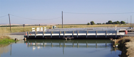
While ASTM A1010 steel has been mostly used in constructing rail cars to carry corrosive coal, in 2004, a bridge was built with the steel and placed in service. The bridge is an innovative multicell bridge girder design installed in Colusa County, CA (see figure 1).(7) Constructed of ASTM A1010 grade 50 steel, the bridge was one of California's Innovative Bridge Research and Construction Program projects in 2002. ASTM A1010 steel was chosen because of its exceptional atmospheric corrosion resistance, allowing it to eliminate the corrosion allowance for the structure, thereby reducing the steel thickness to only 0.16-inches (4 mm).
Figure 1. Photo. Fairview Road Bridge over the Glen-Colusa Canal in Colusa, CA.
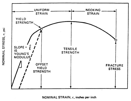
The corrosion-resistant steel is intended to meet the structural performance requirements of grades ASTM A709-50W and/or ASTM A709-70W.(2) The mechanical properties of bridge steels are represented by the yield strength (YS), tensile strength (TS), and tensile elongation (EL). Figure 2 and figure 3 illustrate the essential features of the tensile test. The 0.2 percent YS is measured by drawing a line parallel to Young's modulus at a distance on the x-axis representing 0.2 percent nominal strain, noting the intersection point with the measured curve. EL is determined on a broken tensile specimen by comparing the final gauge length (Lf in figure 3) with the initial gauge length (L0 in figure 3). Design engineers determine the thickness of the steel bridge structural members by employing stress calculations based on the dead weight of the bridge plus live loads during bridge service. Steel bridge durability depends in part on the steel thickness remaining constant during the bridge life.
1 psi = 6.89 kPa
1 inch = 25.4 mm
Figure 2. Illustration. Stress strain curve of tensile test.
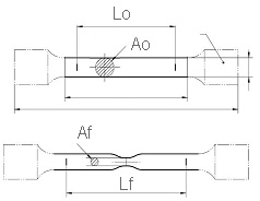
A0 = Tensile specimen original cross sectional area.
Af = Tensile specimen final cross sectional area.
Figure 3. Illustration. Round tensile specimen before tensile test.
The impact toughness of bridge steel is not a direct design characteristic of bridges. Instead, impact toughness is used as a quality control measure to confirm that the steel was correctly manufactured. The minimum absorbed energy of a set of three Charpy V-notch (CVN) impact specimens is specified by the bridge steel standards. In the case of the present study, the requirements are shown in table 1.
Table 1. Mechanical properties of ASTM A1010 production plates and specified minimum properties for ASTM A709-50W and A709-70W in nonfracture critical (NFC) bridge design elements.
Steel |
0.2 Percent |
TS (ksi) |
El (percent) |
Longitudinal Charpy |
LCVN |
ASTM A1010 Production |
56.7 |
76.7 |
36 |
162 |
154 |
ASTM A709-50W |
> 50 |
>70 |
> 21 |
> 20 |
NR |
ASTM A709-70W |
> 70 |
85–110 |
> 19 |
NR |
> 25 |
1 ksi = 6.89 MPa °C = (°F-32)/1.8 1 ft-lb = 1.3558 J NR = No requirement. |
|||||
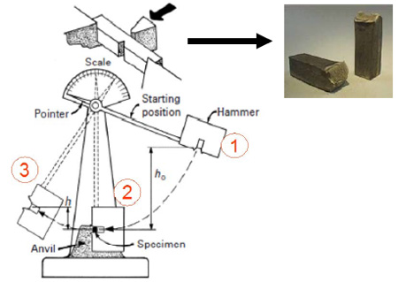
Figure 4 shows a broken standard CVN test specimen that, before testing, measured 0.394 x 0.394 x 2.165 inches (10 x 10 x 55 mm). The figure also shows a sketch of the pendulum machine in which the CVN test is performed. At position 1, the hammer has a potential energy determined by its mass and original height (h0). At position 2, the hammer potential energy is converted fully to kinetic energy immediately before it impacts the Charpy specimen. Position 3 illustrates the hammer position after the specimen fracture. The final potential energy is determined by the final height, h, and the energy absorbed by the Charpy specimen is determined by the mass of the hammer and the difference between h0 and h.
Before the specimen is placed in the machine, it is chilled to the required test temperature. The test temperature is important because bridge steels undergo a transition in fracture behavior as the test temperature decreases. The Charpy requirements depend on whether or not the bridge element is fracture critical (FC).(2) For NFC applications, the Charpy test temperatures prescribed in ASTM A709 are 10 °F (-12 °C) and -10 °F (-23 °C) for grades 50W and 70W, respectively. Recent production experience for ASTM A1010 steel is shown in table 1 for 1,243 T (1,128,000 kg) of production plates.
Figure 4. Illustration. Charpy impact test machine and broken specimen.
For purposes of this study, the goal of the new improved corrosion-resistant steel is to exceed the minimum requirements as currently stipulated in ASTM A709 for NFC grades 50W and 70W and to be comparable to (or superior to) the required properties in table 1.(2)
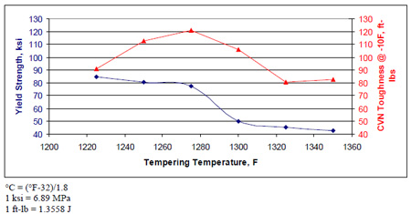
To achieve these mechanical properties, the rolled steel may be heat treated by normalizing and tempering. Normalizing steel involves placing the steel plate in a furnace and heating it to a temperature greater than the critical temperature for the particular grade of steel. The crystal structure changes from its room temperature form to its high-temperature form called austenite. The plate is then removed into still air and is cooled naturally. During cooling, the steel crystal structure transforms from austenite to one of several possible room temperature forms. Tempering is a process where the normalized steel is reheated to a temperature below the critical temperature for the steel. Tempering causes the steel to become softer, and its YS and TS diminish. Tempering changes the strength/impact toughness balance of all steels, including ASTM A1010. Figure 5 shows the results of a tempering study conducted on 2.5-inch (63.5-mm)-thick ASTM A1010 steel. In this case, tempering the steel at temperatures as high as 1,280 °F (693 °C) provided a 70-ksi (483-MPa) minimum YS, while the Charpy impact toughness greater than 80 ft-lb (108 J) was greater than the 25 ft-lb (34 J) needed for NFC bridge members. Similar tempering studies were performed to confirm whether any newly developed steel met the requirements in table 1.
Figure 5. Graph. Effect of tempering temperature on YS and Charpy impact toughness of ASTM A1010 steel.
Fabrication of steel bridges requires excellent weldability to keep construction costs to a minimum. The weldability of ASTM A1010 has been studied extensively, and the steel is readily weldable by flux core arc welding, gas metal arc welding, shielded metal arc welding, and gas tungsten arc welding processes employing austenitic stainless steel filler metal.(8) High heat input submerged arc welding is also possible after verifying that the post-weld mechanical properties are suitable for application. Preheating before welding is necessary to eliminate surface moisture. The principle reason for the good weldability of ASTM A1010 is its low carbon (C) content, with typically less than 0.02 percent C. The proposed new steels all contain less than 0.02 percent C to assure their good weldability.
The atmospheric corrosion performance of structural steels for bridges has been measured using many methods. The most common representation of steel corrosion is reported as thickness loss per surface. This is determined by measuring the mass loss of a sample divided by the surface area of the sample. The resulting value is reported as thickness loss, but it is understood to mean the average thickness loss per surface. This terminology will be used throughout this report.
Thickness loss of exposed test coupons and spectroscopic analysis of the corrosion products are commonly used in tandem to evaluate the corrosion performance of steel. Both of these characterizations were used in this study to quantify and understand the corrosion properties of the various steels and to evaluate how the corrosion properties are affected by different environmental conditions that bridges are exposed to in chloride-containing locations.
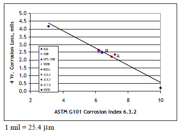
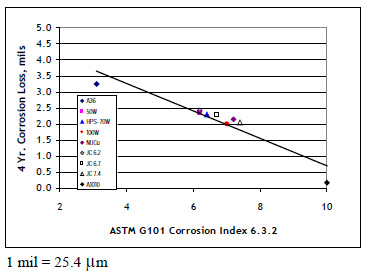
As illustrated in figure 6 and figure 7, the corrosion behavior of plain carbon steel (designated in the figures as A36), low alloy (weathering) steels, and ASTM A1010 stainless steels in coastal atmospheric corrosion has been shown to be reasonably well predicted by ASTM G101 corrosion index (CI) 6.3.2.(9) This dimensionless CI is calculated by applying the chemical composition of the steel to an algorithm in ASTM G101. Most weathering steels have a CI between 6 and 7.(4) It is reasonable to conclude that to achieve significantly better chloride-containing atmospheric corrosion resistance than weathering steels, a candidate steel should have a CI close to 10. ASTM A1010 steel has a CI value of 10. The approach used in this study was to design steels with a CI greater than 9.5. This was accomplished by varying the concentration of alloying elements in the new steels with the calculated index from ASTM G101.(9) The idea was to reduce the Cr content and, therefore, the cost of ASTM A1010 steel.
Determination of the corrosion rates of the candidate steels after corrosion exposure in accelerated tests and at a standard U.S. test site was a central component of this project. Historically, a corrosion test site on the Atlantic Ocean in Kure Beach, NC, has been a standard U.S. test site. There are two test lots at Kure Beach. One is located 82 ft (25 m) from the mean high water mark, while the other is 656 ft (200 m) from the water's edge. These lots are designated the 82- and 656-ft (25- and 200-m) lots, respectively (see figure 6 and figure 7).
Figure 6. Graph. 4-year thickness loss at the 82-ft (25-m) lot in Kure Beach, NC.
Figure 7. Graph. 4-year thickness loss at the 656-ft (200-m) lot in Kure Beach, NC.
The thickness loss for weathering steel ASTM A588B, (ASTM G101 CI of 6.2), exposed at the 82-ft (25-m) lot in Kure Beach, NC, averages approximately 0.6 mil per year (mpy) (15.24 m per year).(10) This is about twice the generally accepted maximum corrosion rate for weathering steel structures less than 0.25 mpy (6.35 m per year). In another field corrosion test site, weathering steel coupons were exposed on racks mounted to the underside of Moore Drive Bridge in Rochester, NY, which is 25 years old. The Moore Drive Bridge is in an area of high deicing salt usage on the interstate highway passing beneath the bridge. Following 4 years of exposure, ASTM A588B coupons had experienced thickness loss of 10 mil (254 m), or a rate of 2.5 mpy (63.5 m per year), which is 10 times the generally accepted maximum rate for weathering steel.(11) This corrosion rate approximately agrees with the measured thickness loss of the lower flanges on the Moore Drive Bridge of about 0.14 inches (3.56 mm) but is about five times the rate of thickness loss measured at the 82-ft (25-m) lot in Kure Beach, NC. Spectroscopic analysis shows that the protective patina containing nanophase goethite does not form on the exposed coupons at the Moore Drive Bridge due to the high deicing salt deposition.(11)
The marine chloride deposition at the 82-ft (25-m) lot in Kure Beach, NC, is about 0.118 oz per inch2 per day (250 mg per m2 per day), which is essentially the same amount deposited on average on the underside of Moore Drive Bridge.(12) The reason the corrosion rate is five times higher on the bridge than at Kure Beach is primarily due to the accumulation of salts on the steel flanges and test coupons, a feature not occurring to the boldly exposed test coupons at Kure Beach that experience periodic washing by rain. The Moore Drive Bridge data demonstrate that standard marine coastal test site data are not always indicative of corrosion rates that steel bridge structures may undergo in adverse microclimate situations.
Accelerated corrosion testing in a laboratory is another means by which corrosion rates of test coupons can be measured. Advantages of the laboratory exposures include the reduced time required to observe significant corrosion and the ability to modify the exposure conditions and subsequently determine the corrosion response of the steel. Whereas there are many limitations on the applicability of an accelerated cyclic corrosion test (CCT), one benefit to the procedure is the measurement of the relative corrosion rates of different steels under the same exposure conditions. As such, accelerated CCT was chosen to quickly evaluate the relative corrosion rates of the newly developed steels.
The Society of Automotive Engineers (SAE) J2334 laboratory accelerated CCT was standardized to simulate the corrosion of autobody steel sheet caused by road salts.(13) It involves daily cycles of repeated exposure to dilute salt solution and high and low relative humidity at elevated temperatures. Specifically, for each cycle, the test coupons undergo the salt application stage, where they are placed in a salt solution of 0.5 percent sodium chloride (NaCl), 0.1 percent calcium chloride, and 0.075 percent sodium bicarbonate (buffer) at 77 °F (25 °C) for 15 minutes. Coupons are then exposed to a dry stage of 50 percent relative humidity at 140 °F (60 °C) for 17.75 h, followed by a humid stage of 100 percent relative humidity at 122 °F (50 °C) for 6 h.
To simulate the atmospheric corrosion of bare structural bridge steels in chloride environments, the standard J2334 CCT was studied on ASTM A588B weathering steel coupons.(14) Mass loss of weathering steel coupons showed that 80 test cycles corresponded to an 11-year total thickness loss of 1 mpy (25.4 m per year) at the Kure Beach 82-ft (25-m) marine location. However, the chloride levels on the SAE J2334 test coupons were an order of magnitude lower (0.1 weight percent) than measured on the bridges, and the rust composition in the preliminary tests subsequently lacked akaganeite in the bridge rusts. Spectroscopic analysis of the SAE J2334 coupons showed that the rust formed was maghemite, an iron oxy-hydroxide known to form due to high time-of-wetness, which dominates the corrosion in low chloride locations.
Modifications to the original SAE J2334 solution chemistry (the chloride concentration was increased by a factor of 10 to 5 percent NaCl) were made.(14) The modified J2334 CCT was successful in forming akaganeite on the bare weathering steel. The chloride in the rust was measured to be 2 percent, the same as the rust on the Moore Drive Bridge. Therefore, successful simulation of the under-bridge environment in adverse locations of high chloride deposition was achieved with the modified J2334 CCT. As a result of this preliminary research, the use of the modified SAE J2334 CCT shows promise for simulating structural steel exposures in adverse environments containing high chloride concentrations and high time-of-wetness.
One limitation of test site coupon exposure projects is the significant time, typically greater than 5 years, needed to expose the coupons to measure meaningful trends in the mass loss as rust forms. To some extent, this is now circumvented by either x-ray, micro-Raman, or Mössbauer spectroscopy to identify the corrosion products forming in early exposure periods. Such data can quickly determine formation, or lack thereof, of the most effective protective patina (mainly nanophase goethite) on weathering steel, and thereby predict long-term corrosion rates of the test steel. It is important to analyze the corrosion products on exposed steel by suitable spectroscopy.(5)
The current study was based on the objective of modifying the composition of ASTM A1010 steel to lower its cost of production without significantly reducing its chloride-containing atmospheric corrosion resistance, while achieving the strength and impact toughness required by ASTM A709.
ASTM A1010 steel exhibits a dual-phase microstructure of ferrite plus martensite. To obtain this particular microstructure, the composition of the steel must be carefully balanced. In high-Cr steels, some alloying elements (e.g., nickel (Ni), C, nitrogen (N), manganese (Mn), and copper (Cu)) promote the formation of austenite, while others (e.g., Cr, molybdenum (Mo), vanadium (V), silicon (Si), aluminum (Al), and titanium) promote the formation of ferrite.(15) Modifying ASTM A1010 steel to reduce its manufacturing cost, which was the approach taken in this project, must take into account the changed phase balance between austenite and ferrite so that comparable microstructures, mechanical properties, and weldability can be expected. Simply reducing the Cr content of ASTM A1010 steel unbalances the ferrite-austenite phase mixture. As a result, compensating changes must be made to other alloying elements in the steel. To achieve the 50- and 70-ksi (345- and 482-MPa) targeted YS, the compositions were designed to have either a fully martensitic or a dual phase (martensite plus ferrite) microstructure.
The alloy design selected to reduce the cost of ASTM A1010 steel containing 11 percent Cr was to reduce the Cr content to 9, 7, and 5 percent. To compensate for the concomitant diminished corrosion resistance as estimated by ASTM G101, additions of 2 percent Si, 2 percent Al, or a combination of 2 percent Si plus 2 percent Al were made in the lower percentage Cr experimental steels. Table 2 shows the nominal composition of each experimental steel and its associated CI. All steels contain nominally 0.015 percent C, 1.29 percent Mn, 0.022 percent phosphorus (P), 0.004 percent sulfur (S), 0.08 percent Cu, 0.43 percent Ni, 0.24 percent Mo, 0.020 percent V, 0.005 percent tungsten, 0.014 percent cobalt, 0.001 percent arsenic, 0.002 percent tin, and 0.0150 percent N.
Table 2. Target compositions of experimental steels.
Steel |
Cr |
Si |
Al |
CI |
11Cr |
11.43 |
0.54 |
0.007 |
9.98 |
9Cr |
9.00 |
0.54 |
0.007 |
9.95 |
9Cr 2Si |
9.00 |
2.00 |
0.007 |
9.98 |
7Cr 2Al |
7.00 |
0.54 |
2.000 |
9.86 |
7Cr 2Si |
7.00 |
2.00 |
0.007 |
9.95 |
5Cr2Al2Si |
5.00 |
2.00 |
2.000 |
9.87 |
All of the steels have a CI greater than 9.5 as calculated by ASTM G101.(9) As a result, it was expected that comparable atmospheric corrosion resistance may be achieved with the reduced-Cr experimental steels. The question to be determined is how these steels will actually perform in chloride-containing environments.
The historic market price for ASTM A1010 steel plates is significantly higher than the price of ASTM A709-50W. The higher price for ASTM A1010 steel is related to its higher Cr content and other manufacturing features. Improving the atmospheric corrosion resistance of any uncoated steel (compared to existing weathering steels) requires higher alloying levels and, thus, concomitant higher steel manufacturing cost. Reducing the Cr level in the existing ASTM A1010 steel could reduce the steel manufacturing cost and thereby permit a lower selling price. This is the fundamental assumption made by this study. Steel, such as ASTM A1010, that is free of maintenance costs over the life of the bridge should have a significantly advantageous LCC compared to conventional weathering steels that must be painted to perform in a chloride-containing environment. A key element of the current project was to project the LCC of the new steels that are candidates for bridge construction.