U.S. Department of Transportation
Federal Highway Administration
1200 New Jersey Avenue, SE
Washington, DC 20590
202-366-4000
Federal Highway Administration Research and Technology
Coordinating, Developing, and Delivering Highway Transportation Innovations
| REPORT |
| This report is an archived publication and may contain dated technical, contact, and link information |
|
| Publication Number: FHWA-HRT-15-063 Date: March 2017 |
Publication Number: FHWA-HRT-15-063 Date: March 2017 |
The prevalence of dynamic conditions shown in the LTPP database, as discussed in chapter 3 and in the FWD tests conducted on Waverly Road (near Lansing, MI) as part of this project, emphasized the necessity of using a time-domain based dynamic solution that could also model the viscoelastic response of the HMA layer(s). A new forward dynamic viscoelastic time-domain solution was implemented based on the solution developed by Lee.(98) The new code was written in-house by the research team using the MATLAB® environment and coded for parallel processing to achieve better computational efficiency. This new version of the program is referred to as ViscoWave-II. In addition, a dynamic backcalculation program using ViscoWave‑II as its forward engine was developed with GA as its search core. This was done to ensure uniqueness of the backcalculated solution from the search algorithm. This new dynamic backcalculation program with viscoelastic AC layers and damped elastic unbound layers is called DYNABACK-VE.
This chapter first describes in detail the mathematical development of the dynamic viscoelastic time-domain algorithm. It then presents the verification results for the developed algorithm by comparing the simulation results from the developed algorithm to some of the other existing solutions. Later, this chapter describes different backcalculation schemes using the new forward solution developed in this research. Finally, this chapter reports on the backcalculation algorithms tested using theoretically generated deflection time histories and field-measured FWD data collected as part of this project. Note that the current forward solution (ViscoWave-II) can be extended to include nonlinearity of unbound layers. However, when such a forward solution was used in the backcalculation algorithm, computational efficiency decreased significantly and became unreasonable. Therefore, although nonlinearity of unbound layers was considered in chapter 4, it was not investigated in the dynamic analysis for two reasons: (1) unreasonable computational time and (2) lack of development time.
The time-domain dynamic solution (ViscoWave) developed by Lee was selected as the forward solution.(98) The theoretical development for the proposed methodology followed steps similar to those of the spectral element method, which uses the discrete transforms for solving the wave equations.(2,40) However, the new solution used continuous integral transforms (namely Laplace and Hankel transforms) that were more appropriate for transient, nonperiodic signals in the time domain.(3) The new algorithm code was written in both MATLAB® and C++ and coded for serial and parallel processing with and without multithreading to achieve better computational efficiency. This new version of the program is referred to as ViscoWave-II. The new algorithm represents the master curve using Prony series of 14 elements, not including E∞, instead of the power law used in ViscoWave. The algorithm also was changed so that it accepts the input of temperature profile along the viscoelastic layer. Appendix C describes in detail the mathematical development of the new algorithm.
The algorithm was first implemented in MATLAB® so that the computation would run serially. Then, to speed up the computations, two different parallelization schemes were coded and tested using: (1) a local cluster of 8 and 12 cores and (2) a cluster of 60 computers in the High Performance Computing Center (HPCC) network of Michigan State University using the Message Passing Interface (MPI). Subsequently, as is described later in this chapter, the code was rewritten in C++ to speed the computations even further.
The algorithm was used to simulate the behavior of elastic and viscoelastic structures subjected to an FWD loading. In addition, other available solutions were used to simulate the response of the same pavement structures for validation of the ViscoWave-II algorithm. The results of these numerical simulations and the preliminary validation efforts are presented. For viscoelastic simulation, the master curve was fitted using a Prony series of 14 elements, not including E∞.
Simulation of an Elastic Pavement Structure
The properties of the pavement layers used for the elastic analysis are shown in table 33. The FWD loading was idealized to be a half-sine load distributed over a circular area of with a radius of 6inches, a peak magnitude of 9,000 lb, and a duration of 26 ms. The surface deflections were calculated at radial distances of 0, 8, 12, 18, 24, 36, and 60 inches from the center of the loadingplate.
To verify the results from ViscoWave-II, the elastic simulation was also conducted using the axisymmetric spectral element algorithm LAMDA, which was already verified through a comparison with the 3-D FEA solution.(2) A summary of the theory behind LAMDA is presented in chapter 2. The time histories for the resulting surface deflections are shown in figure 149. The figure indicates that ViscoWave-II and LAMDA showed almost identical results, validating the algorithm behind ViscoWave-II.
Table 33. Layer properties for elastic simulation using LAMDA and ViscoWave-II.
| Layer | Elastic Modulus (ksi) |
Poisson’s Ratio | Thickness (inches) |
Unit Weight (pcf) |
|---|---|---|---|---|
| Asphalt | 145 | 0.35 | 6 | 145 |
| Base | 30 | 0.4 | 10 | 125 |
| Subgrade | 15 | 0.45 | Infinity | 100 |

Figure 149. Graphs. Comparison of surface deflections of a layered elastic structure using ViscoWave-II and LAMDA.
Simulation of Viscoelastic Pavement Structures
The viscoelastic simulation was carried out for thin, medium, and thick pavement structures. The layer parameters considered/assumed are presented in table 34. The FWD loading used in this simulation is presented in figure 150, and it was assumed to be uniformly distributed over a circular area with a radius of 6 inches, a peak magnitude of 9,000 lb, and a duration of 35 ms. The surface deflections were calculated at radial distances of 0, 8, 12, 18, 24, 36, 48, 60, and 72 inches from the center of the loading plate. The viscoelasticity of the AC layer was modeled using a Prony series of the simulated master curve presented in figure 151. The results are shown in figure 152
Table 34. Layer properties for viscoelastic simulation using ViscoWave-II.
| Layer | Thickness (inches) |
Modulus (ksi) |
Poisson Ratio |
Unit Weight (pcf) |
|---|---|---|---|---|
| AC (thin) | 3 | Master Curve | 0.35 | 145 |
| AC (medium) | 6 | |||
| AC (thick) | 10 | |||
| Base | 15 | 25.0 | 0.40 | 125 |
| Subgrade | Infinity | 7.0 | 0.45 | 100 |

Figure 150. Graph. Simulated FWD load.

151. Graph. AC layer master curve for viscoelastic simulation.

Figure 152. Graphs. Results from ViscoWave-II for viscoelastic simulations of thin (top), medium (middle), and thick (bottom) pavements.
Another viscoelastic simulation was carried out using the same pavement structure that was used for the previous elastic simulation (table 33) with a couple of exceptions. The viscoelasticity of the AC was modeled using two different creep compliance functions: one that represents low‑temperature behavior (figure 153 (left)) and the other representing high-temperature behavior in which the viscoelastic effects are more pronounced (figure 153 (right)). In addition, for each of the creep compliance functions shown in figure 153, the subgrade layer was first modeled to be a half-space (infinite thickness) and then with a shallow bedrock (infinite stiffness) located 10 ft below the pavement surface (figure 154). To verify the results of the viscoelastic simulation from ViscoWave-II, a commercially available FEA package, ADINA, was used to simulate the dynamic response of the viscoelastic pavement subjected to the FWD loading. Figure 155 shows the geometry and the FEA mesh that was used for the analysis. The simulations using ADINA were reported by Lee.(98) Although the elements in ViscoWave-II assumed that the elements extend to infinity in the horizontal direction and also in the vertical direction for the one-noded element, the FEA simulation was inevitably conducted with a finite geometry. More specifically, the FEA model only extended to 20 ft in the horizontal direction and 41.3 ft in the vertical direction for the simulation of the half-space (figure 155 (top)).

Figure 153. Graphs. Low- (left) and high- (right) temperature AC creep compliance curves used for ViscoWave-II simulation.

154. Diagrams. Schematic of the pavement structure with half-space (left) and bedrock (right).
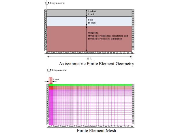
Figure 155. Diagrams. Axisymmetric FEM geometry (top) and FEM mesh (bottom) used for simulation of pavement response under FWD loading.
The FEA mesh was generated in such a way that finer meshes were used near the loaded area, and coarser meshes were used near the geometric boundaries. A total of approximately 8,600 axisymmetric elements, each consisting of 9 nodes, were consistently used for all FEA simulations. The results of the simulations are presented in figure 156 through figure 159. This further verified the implementation of the ViscoWave-II program.

Figure 156. Graphs. Surface deflections of a layered viscoelastic structure with a half-space at low temperature simulated using ViscoWave-II and ADINA.

Figure 157. Graphs. Surface deflections of a layered viscoelastic structure with a bedrock at low temperature simulated using ViscoWave-II and ADINA.

158. Graphs. Surface deflections of a layered viscoelastic structure with a half-space at high temperature simulated using ViscoWave-II and ADINA.

159. Graphs. Surface deflections of a layered viscoelastic structure with a bedrock at high temperature simulated using ViscoWave-II and ADINA.
Simulation of Viscoelastic Pavement Structures With Stiff Soils
The analyses in chapter 3 showed a prevalence of dynamic behavior (in the form of free vibrations of deflection sensor time histories) observed in a large pool of LTPP FWD test data. A sensitivity analysis was then conducted to show that the stiff layer condition did not necessarily correspond to the presence of shallow bedrock, which often lies at much greater depths. Instead, the stiff layer condition can manifest anytime the soils below the subgrade layer are stiffer than that subgrade layer. In this section, the research team describes the investigation using an increasing subgrade modulus with depth instead of a single stiff layer at a fixed depth. The rationale behind this analysis was that in reality, soil profiles generally exhibited increasing soil modulus with depth. This can be due to increased confinement with depth for sands or consolidation level with depth in clay—these situations are very common in any soil profile. This is a commonly observed behavior in the geotechnical engineering profession.
The viscoelastic simulation was carried out using the pavement structure presented in table 35. The FWD loading used in this simulation was assumed to be uniformly distributed over a circular area with a radius of 6inches, a peak magnitude of 9,000 lb, and a duration of 35 ms. Two cases of stiff soils modeling were simulated. The subgrade layer was first modeled to be with a shallow stiff layer (2,000,000 psi) located at about 9 ft below the pavement surface (base case scenario), and then with soils having E-values increasing with depth (figure 160). The surface deflections were calculated at radial distances of 0, 8, 12, 18, 24, 36, 48, 60, and 72 inches from the center of the loading plate. The viscoelasticity of the AC was modeled using a Prony series of the master curve presented in figure 161 (top). The AC layer was divided into two layers with different temperatures as shown in figure 161 (bottom). In addition, the roadbed soil was divided into 11 sublayers of 50 ft total depth (a 2-ft top layer representing the compacted subgrade layer and 10 sublayers of 4.8 ft each with stiffness increasing as a function of depth). The results of the simulations are presented in figure 162. The results indicate that (1) the deflection amplification was higher when a stiff layer modulus was fixed as a high value as opposed to increasing with depth, and (2) the free vibrations (at the tail of the deflection pulses) were lower when the soil modulus was gradually increasing with depth.
Table 35. Layer properties for viscoelastic simulation of structure with stiff soils.
| Layer | Elastic Modulus (psi) |
Poisson’s Ratio | Thickness (inches) |
Unit Weight (pcf) |
|---|---|---|---|---|
| Asphalt | Master curve | 0.35 | 4 | 145 |
| Base | 20,000 | 0.4 | 6 | 125 |
| Subgrade | 13,500 | 0.45 | 600 | 100 |

Figure 160. Diagram. Pavement structure with soils having E-values increasing with depth.

161. Graph and Diagram. AC layer parameters.

Figure 162. Graphs. Surface deflections of pavement structure with shallow stiff layer and soils having E-values increasing with depth.
All the simulations previously described in this chapter were run both serially (ViscoWave) and using parallel computing (ViscoWave-II). Note that the efficiency of ViscoWave-II using the MPI parallelization scheme was only an estimate. Because the program was written in MATLAB®, the parallelization relied totally on the MATLAB® distributed computing server, which was known to have problems with long jobs. To overcome this problem, the research team re-implemented the algorithm using a low-level programming language (C++). The new code was tested on a four-core central processing unit (CPU) computer, and the runtime with Δt = 0.2 ms was reduced from 9min (540 s) to 0.5 min (30 s) in serial (CPU) computing. This represented an 18-fold reduction in computational time. Table 36 presents the computation time for each simulation. It is clear that significant computational savings were achieved when using parallel computation. ViscoWave-II is 8 times faster when using 8 cores, 12 times faster when using 12 cores, and 60 times faster when using 60 cores (available only through the HPCC housed in the Michigan State University College of Engineering). Also, the reduction in computation time by using the code written in C++ language and rather than MATLAB® is significant (almost half). Computation time could be further reduced by using a 64‑bit machine. The computational efficiency went from 5 min (300 s) to 2.5 min (153 s) in a two-core CPU machine without multithreading.
Table 36. ViscoWave-II computational efficiency.
| Time Step (ms) |
Simulation | Serial Computation1 (s) |
Parallel Computation (s) | ||||||||
|---|---|---|---|---|---|---|---|---|---|---|---|
| MATLAB® | C++ With Multicore | C++ With Multithreading | |||||||||
| 2 cores2 | 4 cores3 | 8 cores3 | 2 cores2 | 4 cores3 | 8 cores3 | 2 cores4 | 4 cores4 | 8 cores4 | |||
| 0.1 | Elastic | 1,800 | 900 | 450 | 225 | 500 | 75 | 38 | 250 | 38 | 20 |
| Viscoelastic three-layer system | 2,100 | 1,050 | 525 | 262 | 584 | 88 | 45 | 295 | 45 | 22.5 | |
| Viscoelastic with shallow stiff layer | 2,593 | 1,297 | 649 | 325 | 720 | 108 | 53 | 360 | 54 | 27 | |
| Viscoelastic with soils stiffening with depth | 3,342 | 1,670 | 836 | 418 | 928 | 139 | 70 | 465 | 70 | 35 | |
| 0.2 | Elastic | 840 | 420 | 210 | 105 | 230 | 35 | 19 | 115 | 17 | 8.5 |
| Viscoelastic three-layer system | 1,080 | 540 | 270 | 135 | 300 | 45 | 22.5 | 150 | 22.5 | 11.5 | |
| Viscoelastic with shallow stiff layer | 1,210 | 605 | 304 | 153 | 336 | 50 | 25 | 169 | 26 | 13 | |
| Viscoelastic with soils stiffening with depth | 1,560 | 780 | 390 | 195 | 435 | 66 | 34 | 218 | 33 | 17 | |
| 1Only MATLAB® was used for serial computation. 2Intel core 2 duo CPU with 2.5 GHz (32-bit CPU). 3Intel core 4 duo CPU with 3.5 GHz (32-bit CPU). 4Two threads per core. |
|||||||||||
As part of this project, FWD tests were conducted at Waverly Road test sections. The FWD was provided by FHWA. Testing included the following:
1. Morning set: Four different sections and four different load levels.
2. Afternoon set: Four different sections and four different load levels.
3. Evening set: Four different sections and four different load levels.
The top AC layer configurations of the four different sections selected for FWD are presented in table 37.
Table 37. Waverly Road pavement section information.
| Station Number | Layer 1 (Thickness) | Layer 2 (Thickness) |
|---|---|---|
| 1 | Crumb rubber modified asphalt (4E03a—CRTB) (2 inches) |
Crumb rubber modified asphalt (4E03—CRTB) (2 inches) |
| 2 | Crumb rubber modified asphalt (4E03—CRTB) (2 inches) |
Control 4E03 (2 inches) |
| 3 | Control 4E03 (2 inches) |
Control 4E03 (2 inches) |
| 4 | Control LVSPb (2 inches) |
Control LVSPb (2 inches) |
| a4E03 = MDOT 4E03 Superpave mix bLVSP = Low-Volume Superpave mix. |
||
During the test, different loads were dropped, and deflection histories at each load level were measured. To measure deflection histories, sensors were kept at specified spacing measured from the loading unit. The FWD test loading system and deflection sensors are shown in figure 163.

Figure 163. Photos. FWD used during the field tests.
Temperature in pavements typically varies with depth, which may significantly affect pavement response. Holes at depths 2, 4, 6, 8, and 10 inches were drilled to measure temperature. The drills were made close to the testing location as shown in figure 164. Temperature measurements were taken each time the test was run. The test load levels, deflection sensor locations, temperature profile, and the peak FWD deflection measurements at stations 1 and 3 are given in appendix D. The research team used only stations 1 and 3 because stations 2 and 4 have an asphalt base with a different mix. Use of the latter would cause a problem for the backcalculation algorithm because it was not designed to backcalculate the modulus of more than one AC layer in the pavement structures with different mixes. The same is true if there were multiple subgrade layers with similar modulus values.

Figure 164. Photo. Illustration of temperature measurement at different depths of the pavement.
In this analysis, the ViscoWave-II program was used to analyze the response under the FWD test for the Waverly Road site (stations 1 and 3). The purpose of the exercise was to verify the observations from measurements with theory. To minimize the trials for a reasonable match, the AC dynamic modulus curves from laboratory tests on cores obtained from the field (and presented in appendix D in the section entitled Laboratory-Measured Results for Waverly Road) were used. The corresponding relaxation modulus curves were fitted with appropriate Prony series. The average AC layer temperature measured in the field was used. The depth to the stiff layer was estimated at 8ft using the Ullidtz analysis procedure (described in chapter 4 in the section entitled Backcalculation of the Viscoelastic Properties of the LTPP Sections Using a Single FWD Test With Known Temperature Profile).(94) Initially, the stiff layer modulus was set at 2 million psi, which was the value used for the static and viscoelastic backcalculation described earlier. The moduli of the unbound layers were varied until a reasonable match was obtained. Table 38 and table 39 show the final pavement stations used in the analysis for stations 1 and 3, respectively. The same pavement cross sections with identical layer properties were then used for running the program LAVA for comparison purposes.
Table 38. Pavement properties used in dynamic analysis of station 1 with ViscoWave-II.
| Layer | Modulus (psi) |
Poisson’s Ratio |
Mass Density (pcf) |
Thickness (inches) |
|---|---|---|---|---|
| HMA | Master curve | 0.35 | 145 | 4 |
| Base | 20,000 | 0.4 | 125 | 6 |
| Subgrade | 13,500 | 0.45 | 100 | 96 |
| Stiff Layer | 2,000,000 | 0.2 | 125 | Infinity |
Table 39. Pavement properties used in dynamic analysis of station 3 with ViscoWave-II.
| Layer | Modulus (psi) |
Poisson’s Ratio |
Mass Density (pcf) |
Thickness (inches) |
|---|---|---|---|---|
| HMA | Master curve | 0.35 | 145 | 4 |
| Base | 15,000 | 0.4 | 125 | 6 |
| Subgrade | 12,500 | 0.45 | 100 | 96 |
| Stiff Layer | 2,000,000 | 0.2 | 125 | Infinity |
Figure 165 and figure 166 show the predicted deflection time histories from ViscoWave-II and LAVA together with measured ones for stations 1 and 3, respectively. Figure 167 shows comparisons of ViscoWave-II and LAVA solutions with measured deflections for station 1 in terms of peak deflections (top graph); ratio of predicted to measured deflections (bottom graph).
The following useful observations were made:

Figure 165. Graphs. Comparison of deflection response from ViscoWave-II and LAVA predictions for station 1.

Figure 166. Graphs. Comparison of deflection response from ViscoWave-II and LAVA predictions for station 3.

Figure 167. Graphs. Comparison of ViscoWave-II and LAVA solutions with measured deflections for station 1.
Because of the prevalence of dynamic behavior (in the form of free vibrations of deflection sensor time histories) observed in the large sample of LTPP FWD test data (as shown in chapter 3 of this report), it was hypothesized that in the great majority of the cases, the stiff layer condition may not correspond to the presence of shallow bedrock. Such bedrock would be highly unlikely given that it typically lies at much greater depths. Instead, the stiff layer condition could manifest anytime the soils below the subgrade layer are stiffer than the subgrade layer itself. This could be caused by increased confinement with depth, overconsolidation, or existence of a shallow groundwater table for example; these situations are very common in any soil profile. This would explain the high percentage of sections from the LTPP database that showed dynamic behavior.
Given that argument, the research team decided to conduct a small sensitivity analysis on the value of the stiff layer modulus. This value was reduced from the initial value of 2 million psi, first in 200,000-psi increments (i.e., 1.8 million, 1.6 million psi, etc.), then in 20,000-psi increments below 200,000 psi (i.e., 180,000, 160,000 psi, etc.), and finally used a minimum value of 10,000 psi, which was lower than the subgrade modulus (taken as 13,500 psi).
Figure 168 shows example deflection time histories with the stiff layer modulus decreasing from 2 million to 10,000 psi. The figure shows that the sensors close to the load were mostly not affected by the stiff layer modulus value while those farther from the load were. Free vibrations, while decreasing in magnitude and delayed further, will occur even at low values of the stiff layer modulus, as long as this value is higher that the subgrade modulus value.
Figure 169 and figure 170 summarize the sensitivity analysis results for all sensors in terms of (1) the ratio of predicted to measured peak deflection values and (2) the amplification factor relative to the base case of 2 million psi. The figures show that only the farther sensors (6 through 8) were affected by the stiff layer modulus value and that the effect became visible when the stiff layer modulus was 200,000 psi or lower (compared with the base case of 2 million psi). The effect is significant for the farther sensors, with up to a 50-percent error in the ratio of predicted to measured value and up to a factor of 2 for the amplification ratio, for the lower stiff layer modulus values. Even though these observations used one structure, they could be generalized.
The results of the above analyses clearly showed the superiority of a fully dynamic solution with a viscoelastic AC layer modulus in predicting deflection responses that were in line with the physical reality, as evidenced by the close match in the details of the deflection time histories between theory and observation.

Figure 168. Graphs. Example time histories from ViscoWave-II with decreasing stiff layer modulus and measured sensor deflections for station 1.

Figure 169. Graph. Effect of stiff layer modulus on ratio of predicted to measured sensor deflections for station 1.

Figure 170. Graph. Effect of stiff layer modulus on predicted sensor deflection amplification for station 1.
As discussed in chapter 4, one of the problems with gradient-based methods is that the multidimensional surface represented by the objective function may have many local minima. As a result, the program may converge to different solutions for different sets of seed moduli, as is discussed later in this chapter. The key disadvantages of gradient-based methods are precisely the strengths of the other two categories. In principle, GAs and direct search methods find a global optimum. The key disadvantage is that they can converge very slowly, especially near an optimum, requiring numerous calls to the dynamic forward solution. A second weakness is that determining a termination criterion is not straightforward.
These strengths and weaknesses are considered in choosing an optimization algorithm. A key tradeoff is between the possibility of converging to a local minimum using gradient-based methods and the high computational cost of the GA. The more frequently the algorithm is to be used, the more beneficial the gradient-based algorithm becomes. Therefore, the research team decided to use a hybrid approach—use GA to obtain a good set of seed values that would then be used by the modified LM gradient-based algorithm to backcalculate the master curve of HMA layers and the layer properties for base and subgrade.
The forward solution used a Prony series with 14 coefficients to model the master curve in the Laplace domain. Considering the Prony coefficients as unknown parameters during the backcalculation increased the search domain; thus, it may take a longer time to converge. Therefore, during the backcalculation, Prony series was first fitted to a sigmoidal function using nonlinear least squares optimization. The equation shown in figure 171 presents the fitting steps.(98) Using this approach, the research team had 6 unknowns instead of 17 for the master curve. Table 40 identifies the type of variables for the backcalculation. The equation shown in figure 172 presents the formulation of the optimization problem.

Figure 171. Equation. Fitting steps of the Prony series.
Table 40. Known and unknown parameters.
| Known Parameters | Backcalculated Parameters |
|---|---|
| Thickness of each layer | Master curve coefficients (c1, c2, c3, c4) |
| Poisson’s ratio of each layer | Master curve shift factors (a1, a2) |
| FWD load and setup | Moduli of base, subbase, subgrade, stiff layer |
| Mass density of each layer | Thickness of subgrade if stiff layer exists |

Figure 172. Equation. Optimization problem.
Where:
m = Number of sensors
di = Input deflection information obtained from field at sensor k.
dok = Output deflection information obtained from forward analysis at sensor k.
n = Total number of deflection data points recorded by a sensor.
ci = Sigmoid coefficients.
Eb and Esg = Base and subgrade moduli.
ai = Shift factor polynomial coefficients.
The superscript l represents the lower limit, and u superscript represents the upper limit. Table 41 presents bounds of the variables used as input to the backcalculation algorithm.
Table 41. Bounds of the variables.
| Variable | Lower Limit | Upper Limit |
|---|---|---|
| c1 | 0.045 | 2.155 |
| c2 | 1.800 | 4.400 |
| c3 | -0.523 | 1.025 |
| c4 | -0.845 | -0.380 |
| a1 | -0.00053801 | 0.00113610 |
| a2 | -0.159792 | -0.077 |
| a3 | 1.656202 | 2.763 |
| Ebase(psi) | 10,000 | 30,000 |
| Esubgrade(psi) | 5,000 | 20,000 |
To check the accuracy and robustness of the backcalculation using the new dynamic forward solution, the research team first used only GA and did not focus on the computational efficiency of the algorithm. The verification and evaluation of the new backcalculation program DYNABACK-VE was carried out for the following:
Backcalculation Using Simulated Deflections
This section describes the results of backcalculation using simulated deflections.
Sensitivity Analysis: Sensitivity analysis was conducted to assess the optimal number of populations and generations to be used for backcalculation. The pavement structure used in that sensitivity analysis is presented in table 42. The population-generation combinations used were 30/15, 70/15, 100/15, 200/15, and 300/15. Figure 173 and table 43 summarize the results of the backcalculation. Based on the sensitivity analysis, the optimal population/generation combination was 200/15. Therefore, all the following backcalculations were performed using a population size of 200 with 15 generations. Because the optimal numbers of populations and generations were affected by the number of unknown variables and how smooth the objective function was, the recommendation to use a population size of 200 with 15 generations held true for all cases with 10 or fewer unknowns.
Table 42. Layer properties for the simulated pavement structure.
| Layer | Elastic Modulus (psi) | Poisson’s Ratio |
Thickness (inches) |
Unit Weight (pcf) |
|---|---|---|---|---|
| Asphalt | Master curve (figure 161 (top)) (86.9 °F, 79.3 °F) |
0.35 | 4 | 145 |
| Base | 20,000 | 0.4 | 6 | 125 |
| Subgrade | 13,500 | 0.45 | 96 | 100 |
| Stiff layer | 2,000,000 | 0.25 | Infinity | 125 |

Figure 173. Graph. Backcalculated master curve for different population-generation combinations optimization problem.
Table 43. Backcalculated layer moduli.
| Layer | Elastic Modulus (psi) |
Backcalculated Moduli (psi) for Various Population Sizes | ||||
|---|---|---|---|---|---|---|
| 35 | 70 | 100 | 200 | 300 | ||
| Base | 20,000 | 13,857 | 15,315 | 16,281 | 16,736 | 20,246 |
| Subgrade | 13500 | 6,886 | 11,027 | 13,928 | 13,548 | 13,559 |
| Stiff layer | 2,000,000 | 1,381,454 | 1,473,155 | 1,573,994 | 1,824,154 | 1,591,451 |
Backcalculation of Layer Moduli Only: The viscoelastic simulation was carried out using the same pavement structure presented in table 42. The FWD loading used in all simulations was assumed to be uniformly distributed over a circular area with a radius of 6 inches, a peak magnitude of 9,000 lb, and a duration of 35 ms (same pulse as figure 150). Two cases of stiff soils modeling were simulated. The subgrade layer was first modeled to be with a shallow stiff layer (2 million psi) located at about 8 ft below the pavement surface (figure 174 (left)) and then with subgrade having E-values increasing with depth (figure 174 (right)). The surface deflections were calculated at radial distances of 0, 8, 12, 18, 24, 36, 48, 60, and 72 inches from the center of the loading plate. The viscoelasticity of the AC was modeled using a Prony series of the master curve presented in figure 175 (left). The AC layer was divided into two layers with different temperatures as shown in figure 175 (right). In the backcalculation, the two AC layers were considered to have the same master curve coefficients but different shift factors (computed using the same shift factor coefficients and different temperatures). In addition, for the case where E‑values are increasing with depth (figure 174 (right)), the subgrade layer was divided into 11 sublayers of 50-ft total depth (a 2-ft top layer representing the compacted subgrade layer and 10 sublayers of 4.8 ft each with stiffness increasing as a function of depth). The semi-infinite layer in the case where the subgrade had E-values increasing with depth was a half-space. Therefore, the modulus of the half-space was the same as the lowest sublayer.

Figure 174. Diagrams. Schematic of the pavement structure with stiff soils.

Figure 175. Graph and Diagram. AC layer master curve and temperature profile.
Table 44 shows the viscoelastic dynamic backcalculation results of the pavement structure presented in table 42. Figure 176 shows the errors in deflection time histories. Figure 177 shows the backcalculated relaxation modulus master curve and the corresponding error. Note that the symbols in the plot show the useful range of reduced time for the temperatures in the upper and lower halves of the AC layer. The results were quite reasonable, except for the tail end of the E(t) curve (longer reduced time range). Note that the next section of this chapter describes the results when the research team ran a second backcalculation using the best 100 populations from run 1 as seed values in run 2—the backcalculation of the AC relaxation modulus curve greatly improved.
Table 44. Backcalculated layer moduli.
| Parameter | Simulation | Backcalculated |
|---|---|---|
| c1 | 1.271 | 1.55083 |
| c2 | 2.883 | 2.64494 |
| c3 | 0.22 | 0.04296 |
| c4 | -0.497 | -0.441535 |
| a1 | 0.000442 | 0.000483158 |
| a2 | -0.132 | -0.139815 |
| a3 | 2.34 | 2.68989 |
| Ebase(psi) | 20,000 | 20,246 |
| Esubgrade(psi) | 13,500 | 13,559 |
| Estiff (psi) | 2,000,000 | 1,591,450 |

Figure 176. Graphs. Error in the backcalculated time histories by sensor—backcalculation of layer moduli only.

Figure 177. Graphs. Backcalculation results of the master curve—backcalculation of layer moduli only.
Backcalculation of Layer Moduli and Subgrade Thickness: This section presents the results of the team’s effort to backcalculate the depth to the stiff layer in addition to the stiff layer modulus. The previous profile was used with similar input parameters with the exception of the subgrade thickness, which was unknown and needed to be backcalculated. The backcalculation algorithm was run twice. The final population of the last run was input as the initial population for the second run. Table 45 shows the viscoelastic dynamic backcalculation results. Figure 178 shows the percent error of the deflection time histories. Figure 179 shows the backcalculated relaxation modulus master curves and the corresponding percent error. It was clear that running a second backcalculation using the results from the first run as seed populations led to a much improved backcalculated AC modulus master curve. Note that the curves with circular and triangular symbols in figure 177 show the useful range of reduced time for the temperatures in the upper and lower halves of the AC layer.
Table 45. Backcalculated layer moduli and subgrade thickness.
| Parameter | Simulation | Backcalculated |
|---|---|---|
| c1 | 1.271 | 1.304318 |
| c2 | 2.883 | 2.950314 |
| c3 | 0.22 | 0.107608 |
| c4 | -0.497 | -0.40963 |
| a1 | 0.000442 | 0.000489292 |
| a2 | -0.132 | -0.15225078 |
| a3 | 2.34 | 2.948735039 |
| Ebase(psi) | 20,000 | 20,568 |
| Esubgrade (psi) | 13,500 | 13,372 |
| hsubgrade (inches) | 96 | 95.5 |
| Estiff(psi) | 2,000,000 | 2,281,374 |

Figure 178. Graphs. Error in the backcalculated time histories by sensor—backcalculation of layer moduli and subgrade thickness.

Figure 179. Graphs. Backcalculation results of the AC master curve—backcalculation of layer moduli and subgrade thickness.
Backcalculation Using Field Data
This section provides an evaluation of the new dynamic viscoelastic backcalculation program DYNABACK-VE using the field FWD test results from the Waverly Road tests conducted as part of this study and from two LTPP sections. As discussed previously, the forward solution used a Prony series with 14 coefficients to model the master curve in the Laplace domain. To reduce the number of backcalculated variables, it was decided to reduce the number of coefficients for the shift factor by one using a simple mathematical transformation.(99) The equations in figure 180 show the old and new equations for shift factor. Figure 180 shows the formulation of the optimization problem.
![]()
Figure 180. Equation. New and old shift factor equations.
For figure 181, it was decided to constraint the sum of the first two coefficients of the master curve instead of constraining the two coefficients to reduce the search domain as explained in chapter 4.
 Click for description
Figure 181. Equation. New optimization problem.
Where:
m = the number of sensors.
di = the input deflection information obtained from the field at sensor k
dok = the output deflection information obtained from forward analysis at sensor k.
n = the total number of deflection data points recorded by a sensor.
ci = the sigmoid coefficients.
Eb and Esg = base and subgrade modulus.
ai = the shift factor polynomial coefficients.
The superscript l represents the lower limit, and u represents the upper limit. Table 46 presents the bounds of the variables used as input to the backcalculation algorithm.
Table 46. Bounds of the variables.
| Variable | Lower Limit | Upper Limit |
|---|---|---|
| c1 | 0.045 | 2.155 |
| c1 + c2 | 3.239 | 4.535 |
| c3 | -0.523 | 1.025 |
| c4 | -0.845 | -0.380 |
| a1 | -0.000536829 | 0.00113638 |
| a2 | -0.140735 | -0.097358 |
| Ebase (psi) | 10,000 | 30,000 |
| Esubgrade (psi) | 5,000 | 20,000 |
Waverly Road: The pavement structure used in the backcalculation is presented in table 47. The AC layer was assumed to have a two-step piecewise temperature profile. Figure 182 shows the two-step temperature profile assumed along the AC layer at station 1 (based on measurement in the field). The field data collected for drop 2 section 1 at 9 a.m. and 1 p.m. were used as input to the GA algorithm in DYNABACK-VE to search for the layer moduli as well as the subgrade thickness. Figure 183 shows the collected data. Using the morning and afternoon data together increased over-determinacy of the problem. However, trying to fit more data at the same time using GA would require increasing the variability in the initial population of the GA; which would mean increasing the number of populations and generations. This would have led to an increase in the computational time of the backcalculation algorithm. Therefore, the research team decided to use only the morning test data in the first run to obtain a good initial population; then the afternoon test data was input to the GA in DYNABACK-VE during the second run, using the final population of the first run, taking advantage of elitism.
Table 47. Known layer properties for Waverly Road.
| Layer | Elastic Modulus (psi) |
Poisson’s Ratio | Thickness (inches) |
Unit Weight (pcf) |
|---|---|---|---|---|
| Asphalt | — | 0.35 | 4 | 145 |
| Base | — | 0.4 | 6 | 125 |
| Subgrade | — | 0.45 | — | 100 |
| Stiff layer | — | 0.25 | Infinity | 125 |
| — Indicates unknown value. | ||||

Figure 182. Diagrams. Waverly Road section 1 temperature profile at 9 a.m. and 1 p.m.

Figure 183. Graphs. Waverly Road FWD time histories for section 1 collected at 9 a.m. and 1 p.m.
Table 48 shows the backcalculated layer parameters from the DYNABACK-VE backcalculation. The results were very promising, indicating good stability and realistic values. The following two interesting facts are worth noting:
Table 48. Backcalculated layer parameters for drop 1 section 1—Waverly Road.
| Parameter | Laboratory Test/ Estimation |
Backcalculated |
|---|---|---|
| c1 | 1.482 | 1.58391 |
| c2 | 2.642 | 2.57049 |
| c3 | 0.417 | 0.3894 |
| c4 | -0.569 | -0.55199 |
| a1 | -6.85E-05 | 0.000916 |
| a2 | -1.06E-01 | -0.1126 |
| Ebase (psi) | 20,000 | 20,482 |
| Esubgrade (psi) | 13,500 | 12,987 |
| hsubgrade (inches) | 96 (1/r method) | 98.7 |
| Estiff (psi) | — | 795,304 |
| — Indicates value was not measured. | ||
Figure 184 shows the backcalculated relaxation modulus master curve and the measured laboratory master curve from laboratory testing on field cores. Figure 185 shows the corresponding percent error. Figure 186 and figure 187 show the measured and predicted deflection time histories and the corresponding percent errors for the 1 p.m. test, respectively. The backcalculation results were very good. Running a second backcalculation using the results from the first run as seed populations led to a much improved backcalculated AC modulus master curve.

Figure 184. Graph. Backcalculated master curve for Waverly Road.

185. Graph. Error in the backcalculated master curve for Waverly Road.

Figure 186. Graphs. Predicted versus measured deflection time histories by sensor for 1 p.m. test for Waverly Road.

Figure 187. Graphs. Error in the backcalculated deflection time histories by sensor for 1 p.m. tests for Waverly Road.
The significant practical implications from these results are the following:
LTPP Section 350801 Station 1: The Strategic Highway Research Program ID of the selected section is 0801 in New Mexico (State 35). The section was selected because the deflection time histories showed free vibrations at the end of the load pulse, suggesting that there were dynamic effects (the existence of stiff layer) and that the LTPP database included creep data for these sites to allow verification of the backcalculated results. In this analysis, the research team sought to backcalculate the depth to the stiff layer in addition to the stiff layer modulus using DYNABACK-VE. The backcalculation algorithm was run in two steps. The final population of the first step was entered as the initial population to the second step. Table 49 shows the pavement structure of section 350801. The AC layer was assumed to have a two-step piecewise temperature profile, as shown in figure 188. The measured deflection time histories are presented in figure 189. The FWD deflection data obtained from section 350801 showed some waviness at the end of the load pulse suggesting the existence of a stiff layer. Table 50 shows the backcalculated layer parameters from the DYNABACK-VE backcalculation after all the steps of the algorithm. The results, as shown in figure 190 through figure 192 were very promising, indicating good stability and realistic values.
Table 49. Known layer properties for LTPP section 350801.
| Layer | Elastic Modulus (psi) |
Poisson’s Ratio | Thickness (inches) |
Unit Weight (pcf) |
|---|---|---|---|---|
| Asphalt | — | 0.35 | 4.2 | 145 |
| Base | — | 0.4 | 9.7 | 125 |
| Subgrade | — | 0.45 | — | 100 |
| Stiff layer | — | 0.25 | Infinity | 125 |
| — Indicates unknown value. | ||||

Figure 188. Diagram. Temperature profile for LTPP section 350801.

Figure 189. Graph. Measured FWD time histories for LTPP section 350801.
Table 50. Backcalculated layer parameters for drop 1, station 1—LTPP section 350801.
| Parameters | Backcalculated |
|---|---|
| c1 | 1.09999 |
| c2 | 3.401333 |
| c3 | 1.024748 |
| c4 | -0.50124 |
| a1 | 0.001096 |
| a2 | -0.0926 |
| Ebase (psi) | 20,822.38 |
| Esubgrade (psi) | 18,857.25 |
| hsubgrade (inches) | 193.32 |
| Estiff (psi) | 236,363.82 |

Figure 190. Graph. Backcalculation results of the AC master curve for LTPP section 350801.

Figure 191. Graph. Error in the backcalculated master curve for LTPP section 350801.

Figure 192. Graphs. Error in the backcalculated time histories by sensor for LTPP section 350801.
The following two interesting observations are worth noting:

Figure 193. Graphs. Backcalculated versus measured deflection time histories by sensor for LTPP section 350801, station 1.
LTPP Section 350801 Station 8: The deflection time histories of section 350801 station 8 also showed free vibrations at the end of the load pulse. The approach described in the previous section was used to backcalculate the master AC master curve, the moduli of the unbound layers, and the depth to the stiff layer. Table 49 shows the pavement structure of section 350801. For this section, the AC layer was assumed to have a three-step piecewise temperature profile, as shown in figure 194. The measured deflection time histories are presented in figure 195.
Table 51 shows the backcalculated layer parameters from the DYNABACK-VE backcalculation. Recall that the algorithm is minimizing the error on (c1 + c2). Therefore, the evaluation of the backcalculation algorithm should be based on (c1 + c2). The results were very promising, indicating good stability and realistic values. Figure 196 shows the backcalculated relaxation modulus master curves. Figure 197 shows the corresponding percent error. It was clear that running a second backcalculation using the results from the first run as seed populations led to a much improved backcalculated AC modulus master curve. Figure 198 shows the measured and predicted deflection time histories. The backcalculation results were good, although relatively large errors were seen in the farther deflection sensors. The error results were good compared with the results presented in the previous section for station 1. The backcalculation results for station 8 were significantly better than those for station 1. The error was less than 20percent for reduced times up to 104 s (laboratory value of 20,000 psi versus backcalculated value of 24,000 psi at 104 s). Figure 198 shows very good agreement between the measured and predicted deflection histories for station 8, although there was a larger time shift for sensors 6 through 8. It is believed that this could be due to a synchronization problem between the load and deflection measurements.
To summarize, the backcalculation results were very promising, indicating good stability and realistic values. The backcalculation results for the LTPP section, while reasonable, were not as good as those for the Waverly Road section because only one temperature profile was available; using the morning and afternoon data in the Waverly test increased the over-determinacy of the optimization problem.
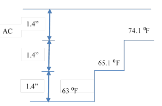
Figure 194. Diagram. Temperature profile for LTPP section 350801.

Figure 195. Graphs. Measured FWD load and deflection time histories for LTPP section 350801.
Table 51. Backcalculated layer parameters for drop 1 station 8 for LTPP section 350801.
| Parameter | Laboratory | Backcalculated |
|---|---|---|
| c1 | 0.120 | 0.804351 |
| c2 | 4.049 | 3.350811 |
| c3 | 1.112 | 0.905003 |
| c4 | -0.423 | -0.48508 |
| a1 | 6.66E-05 | 0.0011361 |
| a2 | -1.41E-01 | -0.13538745 |
| Ebase (psi) | — | 26,183 |
| Esubgrade (psi) | — | 21,579 |
| hsubgrade (inches) | 180 (1/r method) | 185.93 |
| Estiff (psi) | — | 714,658 |
| — Indicates data were not available. | ||

Figure 196. Graph. Backcalculation results of the AC master curve for LTPP section 350801.

Figure 197. Graph. Error in the backcalculated master curve for LTPP section 350801.

Figure 198. Graphs. Backcalculated versus measured deflection time histories by sensor for LTPP section 350801, station 8.
The previous section included a discussion of how conducting two FWD tests in the field with a pavement temperature difference of 50 to 59 °F between the two tests seemed to be sufficient to backcalculate the damaged AC modulus master curve accurately without the need to change the FWD load pulse duration. However, for budgetary and time constraints, it might be impractical to conduct two FWD tests. For these reasons, the research team investigated the effect of increasing the pulse width to increase the useful time range and improve the backcalculation results. However, the team also considered the temperature profile along the AC layer to be able to backcalculate the shift factor coefficients. The effect of using multiple pulses is discussed in appendix B.
The dynamic viscoelastic simulation was carried out using the pavement structure presented in table 52. The FWD loading used in this simulation was assumed to be uniformly distributed over a circular area of a radius of 6 inches, a peak magnitude of 9,000 lb, and pulse durations of 35, 40, 45, and 50 ms (figure 199). The subgrade layer was modeled to be with a shallow stiff layer (2 million psi) located at about 9 ft below the pavement surface (figure 200). The surface deflections were calculated at radial distances of 0, 8, 12, 18, 24, 36, 48, 60, and 72 inches from the center of the loading plate. The viscoelasticity of the AC was modeled using a Prony series of the master curve presented in figure 201 (left). The AC layer was divided into two layers with different temperatures as shown in figure 201 (right). The results of the simulations are presented in figure 202.
Table 52. Layer properties for dynamic viscoelastic simulation.
| Layer | Elastic Modulus (psi) | Poisson’s Ratio | Thickness (inches) |
Unit Weight (pcf) |
|---|---|---|---|---|
| Asphalt | Master curve (86.9 °F) | 0.35 | 2 | 145 |
| Asphalt | Master curve (79.3 °F) | 0.35 | 2 | 145 |
| Base | 20,000 | 0.4 | 6 | 125 |
| Subgrade | 13,500 | 0.45 | 96 | 100 |
| Stiff layer | 2,000,000 | 0.25 | Infinity | 125 |

Figure 199. Graph. Simulated FWD load pulses with various durations.

Figure 200. Diagram. Schematic of the pavement structure with bedrock.

Figure 201. Graph and Diagram. AC layer parameters.

Figure 202. Graphs. Surface deflections of pavement structure for different width of load pulses.
The analysis shows that increasing the width of the FWD pulse would improve the backcalculation of the master curve. However, it would not improve the backcalculation of unbound layer moduli. In the previous section, it was shown that running a second backcalculation using the results from the first run as seed populations not only led to a much improved backcalculated AC modulus master curve but also to much closer base and subgrade moduli. This was because running the second backcalculation after replacing half of the population with random strings increased not only the diversity of the population but the number of generations. As the number of generation increased, the individuals in the population got closer together and approached the minimum point. For all these reasons, the research team recommends increasing the size of the population to 300 when increasing the pulse width instead of testing at different temperatures. Table 53 shows the viscoelastic dynamic backcalculation results of the pavement structure presented in table 52. Figure 203 through figure 206 show the error in the deflection time histories.
Table 53. Backcalculated layer parameters for different pulse durations.
| Parameter | Simulation | Backcalculated | |||
|---|---|---|---|---|---|
| 35 ms | 40 ms | 45 ms | 50 ms | ||
| c1 | 1.271 | 1.606 | 1.501 | 1.404 | 1.359 |
| c2 | 2.883 | 2.405 | 2.550 | 2.677 | 2.796 |
| c3 | 0.22 | 0.323 | 0.302 | 0.286 | 0.152 |
| c4 | -0.497 | -0.595 | -0.582 | -0.574 | -0.526 |
| a1 | 0.00109568 | 1.12E-06 | 0.000163 | 0.000574 | 0.001516 |
| a2 | -0.0925978 | -0.08675 | -0.12647 | -0.09447 | -0.09126 |
| Ebase(psi) | 20,000 | 20,373 | 20,744 | 20,546 | 20,386 |
| Esubgrade (psi) | 13,500 | 15,235 | 16,311 | 17,667 | 14,289 |
| hsubgrade(inches) | 96 | 103.1 | 110.1 | 121.4 | 100.4 |
| Estiff(psi) | 2,000,000 | 773,111 | 607,944 | 701,243 | 898,816 |

Figure 203. Graphs. Error in the backcalculated time histories by sensor for a pulse width of 35 ms.
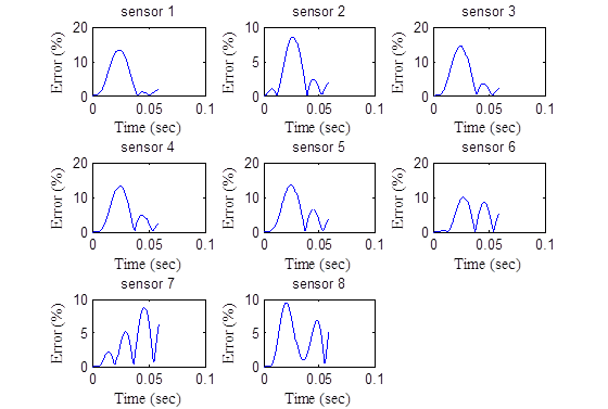
Figure 204. Graphs. Error in the backcalculated time histories by sensor for a pulse width of 40 ms.

Figure 205. Graphs. Error in the backcalculated time histories by sensor for a pulse width of 45 ms.

Figure 206. Graphs. Error in the backcalculated time histories by sensor for a pulse width of 50 ms.
Figure 207 shows the backcalculated relaxation modulus master curve. Figure 208 shows the corresponding error using different pulse widths. The results were quite reasonable, except for the tail end of the E(t) curve (longer reduced time range).

Figure 207. Graph. Backcalculation results of the AC master curve for different pulse widths.

Figure 208. Graph. Error in the backcalculated master curve for different pulse widths.
To conclude, the research team concluded that increasing the pulse width will improve the backcalculation of the master curve, which can be used instead of having to test at multiple temperatures. However, the team also concluded that including a temperature profile is important to be able to backcalculate the shift factors. Two major studies looked at a method to predict the temperature profile using air and pavement surface temperatures. The empirical relationships provided in the LTPP guide and in the Ongel and Harvey study reported errors of 9 and 18 °F, respectively.(5,100) The analysis conducted as part of the current project showed that the temperature gradient in the AC layer is 18 °F at most, which is the same order of magnitude as the error reported by both studies. Therefore, using predicted temperature with depth using such models does not lead to reliable results. It is recommended at this point to use the LTPP manual to manually measure the temperature profile.(5)
Table 54 presents the computation efficiency of the backcalculation algorithm for all the previously discussed analyses. Note that the efficiency of the backcalculation using the MPI parallelization scheme is only an estimate. The algorithm written in MATLAB® was used in all runs.
Table 54. Backcalculation algorithm computational efficiency using GA only.
| Backcalculation | Computational Efficiency | ||
|---|---|---|---|
| Analysis Type | Characteristics | Eight Cores | MPI1 |
| Sensitivity | 35/15 | 5 | 0.67 |
| 70/15 | 11.5 | 1.5 | |
| 100/15 | 17 | 2.25 | |
| 200/15 | 33 | 4.4 | |
| 300/15 | 50 | 6.5 | |
| Simulation | Stiffness and thickness run 1 | 43 | 5.6 |
| Stiffness and thickness run 2 | 44 | 5.8 | |
| Slope run 1 | 75 | 10 | |
| Slope run 2 | 74.5 | 9.9 | |
| Field data | Waverly run 1 | 43.5 | 5.8 |
| Waverly run 2 | 44 | 5.8 | |
| 1Estimated using equal distribution between cores. | |||
In this part of the project, the research team first used GA to obtain a good seed value and to make sure that the algorithm did not converge to a local minimum. Then, the team used the gradient-based LM algorithm to obtain the final results.
Sensitivity Analysis
The research team conducted a sensitivity analysis to select the optimal population/number of generations for the GA and maximum iteration for the LM algorithm. The viscoelastic simulation was carried out using the pavement structure presented in table 55. Figure 209 presents the simulated master curve for the asphalt layer along with the temperature profile. The FWD loading used in all simulations was assumed to be uniformly distributed over a circular area of a radius of 6 inches, a peak magnitude of 9,000 lb, and a duration of 35 ms. Figure 210 (left) presents the simulated FWD load pulse. The subgrade layer was modeled to have a shallow stiff layer (250,000 psi) located at about 8 ft below the pavement surface. The surface deflections were calculated at radial distances of 0, 8, 12, 18, 24, 36, 48, 60, and 72 inches from the center of the loading plate. Figure 210 (right) shows the simulated deflections time histories for all sensors.
Table 55. Layer properties for the simulated pavement structure.
| Layer | Elastic Modulus(psi) | Poisson’s Ratio | Thickness (inches) |
Unit Weight (pcf) |
|---|---|---|---|---|
| Asphalt | Master curve (86.9 °F) | 0.35 | 2 | 145 |
| Master curve (79.3 °F) | 0.35 | 2 | 145 | |
| Base | 20,000 | 0.35 | 6 | 125 |
| Subgrade | 13,500 | 0.45 | 96 | 120 |
| Stiff layer | 250,000 | 0.30 | Infinity | 145 |

Figure 209. Graph and Diagram. AC layer master curve and temperature profile.

Figure 210. Graphs. Simulated FWD pulse and deflection time histories.
Table 56 presents the information for all 60 runs (19 LM method runs, 25 hybrid method runs, and 16 GA method runs). The last column for each method shows the total number of calls to the forward solution (ViscoWave-II) and hence gives an indication of computational cost, i.e., the higher the number the higher the computational cost.
It was observed during the sensitivity analysis that the convergence of the backcalculation using only the LM algorithm was not guaranteed. The algorithm was very sensitive to the seed values. If the seed values were close to the real values, the algorithm converged very fast (about 25 iterations). However, when the seed values were picked randomly inside the search domain, the algorithm converged fast to a local solution or sometimes it diverged as shown in figure 211.
Table 56. Runs information for the sensitivity analysis.
| Method | Run Number |
Population Size |
Number of Generations |
Number of Iterations |
Number of Calls to ViscoWave-II |
|---|---|---|---|---|---|
| LM | 1 | — | — | 100 | 100 |
| 2 | — | — | 150 | 150 | |
| 3 | — | — | 200 | 200 | |
| 4 | — | — | 250 | 250 | |
| 5 | — | — | 300 | 300 | |
| 6 | — | — | 350 | 350 | |
| 7 | — | — | 400 | 400 | |
| 8 | — | — | 450 | 450 | |
| 9 | — | — | 500 | 500 | |
| 10 | — | — | 550 | 550 | |
| 11 | — | — | 600 | 600 | |
| 12 | — | — | 650 | 650 | |
| 13 | — | — | 700 | 700 | |
| 14 | — | — | 750 | 750 | |
| 15 | — | — | 800 | 800 | |
| 16 | — | — | 850 | 850 | |
| 17 | — | — | 900 | 900 | |
| 18 | — | — | 950 | 950 | |
| 19 | — | — | 1,000 | 1,000 | |
| GA+LM | 20 | 50 | 5 | 100 | 350 |
| 21 | 50 | 5 | 150 | 400 | |
| 22 | 50 | 5 | 200 | 450 | |
| 23 | 50 | 5 | 250 | 500 | |
| 24 | 50 | 5 | 300 | 550 | |
| 25 | 75 | 5 | 100 | 475 | |
| 26 | 75 | 5 | 150 | 525 | |
| 27 | 75 | 5 | 200 | 575 | |
| 28 | 75 | 5 | 250 | 625 | |
| 29 | 75 | 5 | 300 | 675 | |
| 30 | 100 | 5 | 100 | 600 | |
| 31 | 100 | 5 | 150 | 650 | |
| 32 | 100 | 5 | 200 | 700 | |
| 33 | 100 | 5 | 250 | 750 | |
| 34 | 100 | 5 | 300 | 800 | |
| 35 | 150 | 5 | 100 | 850 | |
| 36 | 150 | 5 | 150 | 900 | |
| 37 | 150 | 5 | 200 | 950 | |
| 38 | 150 | 5 | 250 | 1,000 | |
| 39 | 150 | 5 | 300 | 1,050 | |
| 40 | 200 | 5 | 100 | 1,100 | |
| 41 | 200 | 5 | 150 | 1,150 | |
| 42 | 200 | 5 | 200 | 1,200 | |
| 43 | 200 | 5 | 250 | 1,250 | |
| 44 | 200 | 5 | 300 | 1,300 | |
| GA | 45 | 35 | 5 | — | 175 |
| 46 | 50 | 5 | — | 250 | |
| 47 | 75 | 5 | — | 375 | |
| 48 | 100 | 5 | — | 500 | |
| 49 | 150 | 5 | — | 750 | |
| 50 | 200 | 5 | — | 1,000 | |
| 51 | 250 | 5 | — | 1,250 | |
| 52 | 300 | 5 | — | 1,500 | |
| 53 | 35 | 15 | — | 525 | |
| 54 | 50 | 15 | — | 750 | |
| 55 | 75 | 15 | — | 1,125 | |
| 56 | 100 | 15 | — | 1,500 | |
| 57 | 150 | 15 | — | 2,250 | |
| 58 | 200 | 15 | — | 3,000 | |
| 59 | 250 | 15 | — | 3,750 | |
| 60 | 300 | 15 | — | 4,500 | |
| — Indicates not applicable. | |||||

Figure 211. Graph. Average error in the backcalculated AC layer master curve for all runs in LM method.
The average error (over reduced times from 10-8 to 108 s) in the E(t) master curve was defined in figure 211. The runs in which the algorithm diverged were repeated. Figure 212 shows the results in terms of average errors in E(t) from the DYNABACK-VE. Figure 213 through figure 216 show the results for base, subgrade, and stiff layer moduli as well as the depth to the stiff layer.

Figure 212. Graph. Average error in the backcalculated AC layer master curve for all runs.

Figure 213. Graph. Average error in the backcalculated base layer modulus for all runs.

Figure 214. Graph. Average error in the backcalculated subgrade modulus for all runs.

Figure 215. Graph. Average error in the backcalculated stiff layer modulus for all runs.

Figure 216. Graph. Average error in the backcalculated depth to the stiff layer for all runs.
It can be observed from figure 212 that the average error in backcalculated E(t) was below the maximum acceptable level (American Association of State Highway and Transportation Officials threshold of 7.5 percent) as defined in figure 87 when any of the following options are true:(1)
Next, assuming a maximum tolerable error of 20 and 10 percent for the remaining parameters (base and subgrade layer moduli, stiff layer modulus and depth to the stiff layer, as seen in figure 212 through figure 216), the optimal runs and corresponding minimum number of computations to arrive at an acceptable solution for each search method are shown in table 57. It can be seen that the hybrid GA+LM approach is the best approach; it is guaranteed to converge within the search domain and is the most computationally efficient.
Table 57. Optimal runs for the various search methods.
| Search Method |
10-Percent Error Tolerance | 20-Percent Error Tolerance | ||
|---|---|---|---|---|
| Optimal Run Number |
Number of Calls to ViscoWave-II |
Optimal Run Number |
Number of Calls to ViscoWave-II |
|
| LMa | 17 | 900 | 16 | 850 |
| GA+LMb | 35 | 850c | 30 | 600c |
| GAb | 59 | 3,750 | 56 | 1,500 |
| aConvergence is not guaranteed (depending on seed values). bConvergence is guaranteed (within the search domain). cComputationally most efficient. The time to run ViscoWave-II depends on the speed and number of processors (cores) used during the backcalculation. |
||||
Figure 217 and figure 218 show the measured and predicted deflection time histories for GA+LM runs 30 and 32, respectively, for comparison purposes. Table 58 shows the backcalculation results. The backcalculation results were good, although relatively large errors were seen in the farther deflection sensors. Figure 219 shows the backcalculated relaxation modulus master curves for both combinations. Figure 220 shows the corresponding percent error. Running a GA algorithm along with the LM algorithm led to a much improved backcalculated AC modulus master curve that was achieved faster and more efficiently.

Figure 217. Graphs. Error in the backcalculated deflections for run 30.

Figure 218. Graphs. Error in the backcalculated deflections for run 35.
Table 58. Backcalculated layer parameters for the simulated structure.
| Layer | Simulated | Run 35 | Run 30 | ||
|---|---|---|---|---|---|
| AC | Master Curve Coefficient | Master Curve Coefficient | Error (Percent) | Master Curve Coefficient | Error (Percent) |
| c1 | 1.271 | 1.296 | 1.96 | 1.112 | -12.5 |
| c2 | 2.883 | 2.883 | 0.01 | 3.085 | 7.1 |
| c3 | 0.22 | 0.145 | -33.9 | 0.291 | 32.2 |
| c4 | -0.497 | -0.512 | 3.1 | -0.427 | -14.2 |
| a1 | 0.001096 | 0.000647 | -40.9 | 0.000448 | -59.1 |
| a2 | -0.0926 | -0.09686 | 4.6 | -0.1317 | 42.3 |
| Base, subgrade, and stiff layer | Elastic Modulus (psi) | Elastic Modulus (psi) | Error (Percent) | Elastic Modulus (psi) | Error (Percent) |
| Ebase (psi) | 20,000 | 21,769.7 | 8.8 | 23,797 | 19.0 |
| Esubgrade (psi) | 13,500 | 14,464.4 | 7.1 | 14,473 | 7.2 |
| Estiff (psi) | 200,000 | 331,313 | 32.5 | 349,894 | 40.0 |
| hsubgrade (inches) | 96 | 103.5 | 7.8 | 106.0 | 10.4 |

Figure 219. Graph. Backcalculated master curves for runs 30 and 35.

Figure 220. Graph. Percent error in the backcalculated master curves for all combinations.
Backcalculation Using Field Data
This section presents the evaluation of the new dynamic viscoelastic backcalculation program DYNABACK-VE using the field FWD test results from six LTPP sections. The details of the identified sections are presented in table 59. Table 60 shows the pavement structure of all the identified sections. These sections were identified based on the following criteria:
Table 59. Identified LTPP sections for the verification of DYNABACK-VE.
| State Code |
Section | Date of Construction |
Total Number of Constructions |
Section Type |
Experiment Number |
Test Date |
Test Time |
|---|---|---|---|---|---|---|---|
| 1 | 0101 | 04/28/05 | 1 | SPS | 1 | 04/28/05 | 15:59 |
| 6 | A805 | 11/16/11 | 1 | SPS | 8 | 11/16/11 | 12:23 |
| 6 | A806 | 11/16/11 | 1 | SPS | 8 | 11/16/11 | 13:50 |
| 30 | 0113 | 07/12/10 | 5 | SPS | 1 | 07/12/10 | 09:39 |
Table 60. Layer properties for LTPP sections.
| Section | Property | Asphalt Concrete Layer | Granular Base | Subgrade | Stiff Layer | ||
|---|---|---|---|---|---|---|---|
| Layer 1 |
Layer 2 |
Layer 3 |
|||||
| 10101 | Thickness (inches) | 2.47 | 2.47 | 2.47 | 6 | Semi-infinite | No stiff layer |
| Temperature (°F) | 100.0 | 92.5 | 91.6 | N/A | N/A | ||
| Poisson’s ratio | 0.35 | 0.40 | 0.45 | ||||
| Unit weight (pcf) | 145 | 125 | 100 | ||||
| Relaxation modulus | E(t) coefficients (c1, c2 ,c3, c4) Backcalculated | Backcalculated | Backcalculated | ||||
| a(T) coefficients | (a1, a2)—Backcalculated | N/A | N/A | ||||
| 6A805 | Thickness (inches) | 1.3 | 1.3 | 1.3 | 8.2 | Backcalculated | Semi-infinite |
| Temperature (°F) | 73.6 | 69.1 | 68.2 | N/A | N/A | N/A | |
| Poisson’s ratio | 0.35 | 0.4 | 0.45 | 0.2 | |||
| Unit weight (pcf) | 145 | 125 | 100 | 125 | |||
| Relaxation modulus (ksi) | E(t) coefficients (c1 ,c2, c3, c4) Backcalculated | Backcalculated | Backcalculated | Backcalculated | |||
| a(T) coefficients | (a1, a2) Backcalculated | N/A | N/A | N/A | |||
| 6A806 | Thickness (inches) | 2 | 2 | 2.8 | 12.1 | Backcalculated | Semi-infinite |
| Temperature (°F) | 79.1 | 75.1 | 71.2 | N/A | N/A | N/A | |
| Poisson’s ratio | 0.35 | 0.4 | 0.45 | 0.2 | |||
| Unit weight (pcf) | 145 | 125 | 100 | 125 | |||
| Relaxation modulus (ksi) | E(t) coefficients (c1, c2, c3, c4) Backcalculated | Backcalculated | Backcalculated | Backcalculated | |||
| a(T) coefficients | (a1, a2) Backcalculated | N/A | N/A | N/A | |||
| 300113 | Thickness (inches) | 2 | 2 | 2 | No stiff layer | Semi-infinite | No stiff layer |
| Temperature (°F) | 84.7 | 80.1 | 79.2 | N/A | N/A | ||
| Poisson’s ratio | 0.35 | 0.4 | 0.45 | ||||
| Unit weight (pcf) | 145 | 125 | 100 | ||||
| Relaxation modulus (ksi) | E(t) coefficients (c1 ,c2, c3, c4) Backcalculated | Backcalculated | Backcalculated | ||||
| a(T) coefficients | (a1, a2) Backcalculated | N/A | N/A | ||||
| N/A = Not applicable. | |||||||
In this analysis, the research team sought to backcalculate the depth to the stiff layer in addition to the stiff layer modulus using DYNABACK-VE. The backcalculation algorithm was run in two steps. The final population of the first step was input as initial population to the second step. The AC layer was assumed to have a three-step piecewise temperature profile for all the sections, as shown in table 60.
LTPP Section 10101: The measured deflection time histories from all the drops for section 10101 are presented in figure 221. The deflection time histories did not show waviness at the end of the signal, which indicated that there was no stiff layer or that the depth to the stiff layer was greater than 15 ft. The presence of a stiff layer was further evaluated using the graphical method suggested by Ullidtz.(94) The method involves plotting peak deflections obtained from FWD testing versus the reciprocal of the corresponding sensor location (measured from the center of loading). The analysis showed that a stiff layer existed at 86.9, 32.7, 109.8, and 26.6 ft using the deflection histories from drops 1 through 4, respectively. Even though the 1/r method suggested that there was no stiff layer, the research team decided to include a stiff layer in the pavement structure. The backcalculation results from all the drops are presented in table 61. Figure 222 shows the backcalculated master curves. Figure 223 shows the backcalculated time-temperature shift factors. For section 10101, the backcalculated relaxation modulus master curves from all the drops matched very well with the measured master curve (figure 222). However, it can be seen from figure 223 that the backcalculated shift factor functions for all the drops showed a good match over the temperature range of 50 to 131 °F, whereas the laboratory-measured values deviated from the backcalculated values. This could be because laboratory creep compliance tests are usually not reliable in determining time-temperature superposition properties because a perfect stress-step function is very difficult to achieve in the laboratory and also because the results are contaminated with viscoplasticity, especially at the high temperatures and long creep times.
Table 61. Backcalculation results for LTPP section 10101 using DYNABACK-VE.
| Parameter | Laboratory Results |
Backcalculated Results | ||||
|---|---|---|---|---|---|---|
| Drop 1 | Drop 2 | Drop 3 | Drop 4 | |||
| c1 | 0.304 | 0.420 | 0.402 | 0.431 | 0.391 | |
| c2 | 4.160 | 4.049 | 4.042 | 4.009 | 4.053 | |
| c3 | 0.684 | 0.611 | 0.731 | 0.711 | 0.656 | |
| c4 | -0.428 | -0.442 | -0.450 | -0.457 | -0.418 | |
| a1 | 3.14E-04 | 0.0011364 | 0.0008364 | 0.0010633 | 0.0010246 | |
| a2 | -1.47E-01 | -0.070735 | -0.0587358 | -0.064368 | -0.04627 | |
| Ebase(psi) | — | 28,519 | 23,433 | 20,121 | 20,124 | |
| Esubgrade (psi) | — | 48,899 | 46,669 | 42,889 | 45,371 | |
| hsubgrade (ft) | Drop 1 | 86.9 (1/r) | 25 | 29 | 34.5 | 32.5 |
| Drop 2 | 32.7(1/r) | |||||
| Drop 3 | 109.8(1/r) | |||||
| Drop 4 | 26.6(1/r) | |||||
| Estiff (psi) | — | 814,826 | 922,537 | 732,145 | 655,421 | |
| — Indicates data were not available. | ||||||

Figure 221. Graphs. Measured FWD load and time histories for LTPP section 10101.

Figure 222. Graph. Backcalculated master curves for LTPP section 10101 from all the drops.

Figure 223. Graph. Backcalculated shift factors for LTPP section 10101 from all the drops.
From table 61, the backcalculated moduli for unbound layers from all the drops suggest that the subgrade layer was stiffer than the base layer. Also, it was observed that the backcalculated moduli for the unbound layers were lower as the load level increased, which suggests softening conditions. The same section was used in LTPP data analysis presented in chapter 3. Figure 224 presents the load-to-deflection ratio at each load level. The plots also suggest softening conditions. The practical implication of these observations suggests that one could backcalculate the moduli for the unbound layers from all the drops to capture the nonlinearity. This could merit discussion for future research.

Figure 224. Graph. Softening behavior for LTPP section 10101.
LTPP Section 6A805: The measured deflection time histories from all the drops for section 6A805 are presented in figure 225. The deflection time histories did show waviness at the end of the signal, which indicates that there was a stiff layer. The depth to the stiff layer estimated using Ullidtz method is about 70.4 ft using the deflection histories from drop 1.(94) Even though the 1/r method suggests that there was no stiff layer, the research team also decided to include a stiff layer in the pavement structure. The backcalculation results using drop 1 time histories are presented in table 62. Figure 226 shows the backcalculated and measured master curves. Figure 227 shows the backcalculated and measured time-temperature shift factors. For section 6A805, the backcalculated and the laboratory-measured relaxation modulus master curves matched very well with the measured master curve until reduced time of 10 s (figure 226). However, it can be seen from figure 227 that the backcalculated shift factor functions did not match.
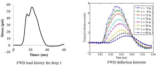
Figure 225. Graphs. Measured FWD load and time histories for LTPP section 6A805.
Table 62. Backcalculation results for LTPP section 6A805 using DYNABACK-VE.
| Parameter | Laboratory Results |
Drop 1 Backcalculation |
|---|---|---|
| c1 | 1.381 | 1.609 |
| c2 | 2.983 | 2.758 |
| c3 | 1.625 | 1.425 |
| c4 | -0.784 | -0.845 |
| a1 | -0.00169 | 0.001 |
| a2 | -0.08729 | -0.077 |
| Ebase (psi) | — | 43,546 |
| Esubgrade (psi) | — | 17,435 |
| hsubgrade (ft) drop1 | 70.4 (1/r) | 14 |
| Estiff (psi) | — | 315,452 |
| — Indicates data values were not measured. | ||

Figure 226. Graph. Backcalculated master curves for LTPP section 6A805.

Figure 227. Graph. Backcalculated shift factors for LTPP section 6A805.
In table 62, the backcalculated depth to the stiff layer is about 14 ft, which suggests that there was a stiff layer at a shallow depth. This contradicts the results from the 1/r method. However, because this estimated depth is close to the depth to the stiff layer beyond which dynamic effects are insignificant, i.e., 15 ft, the possible existence of a stiff layer could be ignored.(96) The load-to-deflection ratio presented in figure 228 shows a maximum slope of about 4 percent seen for sensor 8, which suggests that nonlinearity can be ignored.

Figure 228. Graph. Load-to-deflection ratio for LTPP section 6A805.
LTPP Section 06A806: The measured deflection time histories from all the drops for section 06A806 are presented in figure 229. The deflection time histories did show waviness at the end of the signal, which indicated that there was a stiff layer. Using the Ullidtz method, the depth to the stiff layer was estimated as a negative value, which was interpreted as the absence of a stiff layer.(94) Even though the 1/r method suggests that there was no stiff layer, the research team also decided to include a stiff layer in the pavement structure. The backcalculation results using drop 1 time histories are presented in table 63. Figure 230 shows the backcalculated and measured master curves. Figure 231 shows the backcalculated and measured time-temperature shift factors. For section 6A806, the backcalculated and the laboratory-measured relaxation modulus master curves matched very well with the measured master curve until reduced time of 1 s (figure 230). However, it can be seen from figure 231 that the backcalculated shift factor functions did not match.

Figure 229. Graphs. Measured FWD load and time histories for LTPP section 6A806.
Table 63. Backcalculation results for LTPP section 6A806 using DYNABACK-VE.
| Parameter | Laboratory Results |
Drop 1 Backcalculation |
|---|---|---|
| c1 | 1.157 | 1.252 |
| c2 | 3.356 | 3.259 |
| c3 | 1.388 | 1.025 |
| c4 | -0.673 | -0.723 |
| a1 | -0.0027 | -0.001 |
| a2 | -0.06976 | -0.140735 |
| Ebase (psi) | — | 26,546 |
| Esubgrade (psi) | — | 19,075 |
| hsubgrade (ft) drop 1 | No stiff (1/r) | 13.33 |
| Estiff (psi) | — | 316,575 |
| — Indicates data were not available. | ||

Figure 230. Graph. Backcalculated master curves for LTPP section 6A806.

Figure 231. Graph. Backcalculated shift factors for LTPP section 6A806.
In table 63, the backcalculated depth to the stiff layer is about 13 ft, which suggests that there was a stiff layer at a shallow depth. This contradicts the results from the 1/r method. However, because this estimated depth is close to the depth to the stiff layer beyond which dynamic effects are insignificant, i.e., 15 ft, the possible existence of a stiff layer could be ignored.(95) The load-to-deflection ratio presented in figure 232 shows a maximum slope of about 5 percent seen for only sensor 8, which suggests that nonlinearity can be ignored.

Figure 232. Graph. Load-to-deflection ratio for LTPP section 6A806.
LTPP Section 300113: The measured deflection time histories from drop 1 for section 300113 are presented in figure 233. The deflection time histories did not show waviness at the end of the signal, which indicates that there was no stiff layer or that the depth to the stiff layer was greater than 15 ft. Using the Ullidtz method, the depth to the stiff layer was estimated at about 96.4 ft.(94) Even though the 1/r method suggests that there was no stiff layer, the research team included a stiff layer in the pavement structure. The backcalculation results using drop 1 time histories are presented in table 64. Figure 234 shows the backcalculated and measured master curves. Figure 235 shows the backcalculated and measured time-temperature shift factors. For section 6A806, the backcalculated and the laboratory-measured relaxation modulus master curves matched very well until reduced time of 1 s (figure 234). However, it can be seen from figure 235 that the backcalculated shift factor functions did not match.

Figure 233. Graphs. Measured FWD load and time histories for LTPP section 300113.
Table 64. Backcalculation results for LTPP section 6A806 using DYNABACK-VE.
| Parameter | Laboratory Results |
Drop 1 Backcalculation |
|---|---|---|
| c1 | 0.778 | 1.098 |
| c2 | 3.789 | 3.449 |
| c3 | 0.000 | -0.081 |
| c4 | -0.400 | -0.423 |
| a1 | 4.97E-04 | 0.001 |
| a2 | -1.57E-01 | -0.077 |
| Ebase (psi) | — | 10,745 |
| Esubgrade (psi) | — | 22,995 |
| hsubgrade(ft) drop1 | 96.4 (1/r) | 16 |
| Estiff (psi) | — | 215,298 |
| — Indicates data were not available. | ||

Figure 234. Graph. Backcalculated master curves for LTPP section 300113.

Figure 235. Graph. Backcalculated shift factors for LTPP section 300113.
In table 63, the backcalculated depth to the stiff layer is about 16 ft, which is close to the depth to the stiff layer beyond which dynamic effects are insignificant, i.e., 15 ft.(96) Therefore, the possible existence of a stiff layer could be ignored. Figure 236 shows the load-to-deflection ratio for all the sensors. The maximum slope is about 5 percent for only sensor 7, which means that nonlinearity could be ignored.

Figure 236. Graph. Load-to-deflection ratio for LTPP section 300113.
A new solution and its associated computer program were developed for dynamic viscoelastic time-domain backcalculation of multilayered flexible pavement parameters under FWD tests in the time domain. The method uses a time-domain viscoelastic solution as a forward routine (ViscoWave-II) and a hybrid routine (DYNABACK-VE: GA and modified LM method) for backcalculation analysis. For the GA-based backcalculation procedure, the research team recommends using DYNABACK-VE twice with a population of 200 and 15 generations. When increasing the pulse width, the team recommends using a population of 300 and 15 generations. The advantage of the new solution is that it can analyze the response of pavement systems in the time domain and can therefore accommodate time-dependent layer properties and incorporate wave propagation. Also, because the backcalculation is performed in the time domain, the algorithm is not sensitive to truncation in the deflection time histories. The new algorithm is capable of backcalculating layer moduli, including the master curve of the AC layer at every reduced time and depth to the stiff layer, if it exists, and its modulus value. The results using simulated deflection time histories and field FWD data showed excellent stability and accuracy. Note that the backcalculation algorithm is not designed to backcalculate the modulus of more than one AC layer in pavement structures with different mixes or in cases where there are multiple subgrade layers with similar moduli values.
The sensitivity of dynamic backcalculation solutions to signal noise and synchronization problems is high. The remedy to noise is to preprocess the raw data by filtering out the high-frequency content of the signal (anything above 100 Hz) in deflection and load pulse data. Also, in the analysis presented in chapter 5, the percent error between the computed and measured displacement was used as the minimizing error. If percent error were used as the minimizing objective, it could lead to overemphasis of lower magnitudes of deflections at the later portion of the time history, which typically includes noise and integration errors. Hence another fit function was proposed in which the percent error was calculated with respect to the peak of deflection at each sensor. This de-emphasizes the tail data by normalizing them with respect to the peak.
If synchronization problems occur, the dynamic backcalculation algorithm may not work as well, although one could shift the signals similar to what was done in the quasi-static viscoelastic solution (chapter 4). Because the quasi-static solution presented in chapter 4 is already coded to remove the time delay between sensors, the research team recommends the use of BACKLAVA instead of DYNABACK-VE when such a synchronization problem exists and cannot be removed manually.
The results from dynamic analyses clearly showed the superiority of a fully dynamic solution with a viscoelastic AC layer modulus in predicting deflection responses that are in line with what one would expect from soil, as evidenced by the close match in the details of the deflection time histories between theory and observation. The theoretical predictions from ViscoWave-II showed very good agreement with the measured deflection time histories. The fact that theory and measurement showed the same behavior with time was proof that these observations were physically real. This is important in that it reinforces the following: (1) a comprehensive model that takes into account viscoelasticity of the AC layer, damping in the unbound layers, and dynamics in terms of inertial and wave propagation effects can explain the measured data with all their complexities; and (2) the FWD sensor measurements, if properly calibrated, can show the physical behavior for most of the time range, with the exception of the drift problems at the tail of the records.
In contrast, the layered viscoelastic solution cannot simulate the true deflection time histories because it cannot account for inertial and wave propagation effects. As such, it cannot predict the time delays in the response, the initial rebounds of the farther sensors, and the free vibrations after the load is applied. Also, the layered viscoelastic solution significantly underestimates the deflections when a stiff layer is present. This is because it cannot account for dynamic amplification caused by the wave energy trapped in the unbound layers when a stiff layer condition exists.

