U.S. Department of Transportation
Federal Highway Administration
1200 New Jersey Avenue, SE
Washington, DC 20590
202-366-4000
Federal Highway Administration Research and Technology
Coordinating, Developing, and Delivering Highway Transportation Innovations
| REPORT |
| This report is an archived publication and may contain dated technical, contact, and link information |
|
| Publication Number: FHWA-HRT-15-063 Date: March 2017 |
Publication Number: FHWA-HRT-15-063 Date: March 2017 |
Unbound layers typically exhibit nonlinearity, i.e., their responses are affected by the state of stress. This stress includes the induced stress due to the applied load on the surface and the geostatic stress. Software programs such as KENLAYER and MICHPAVE consider the constitutive equation between resilient modulus and stress invariants as that shown in figure 266.
![]()
Figure 266. Equation. Relationship between resilient modulus and stress invariants.
Where:
θ = σ1 + σ2 + σ3 + γz(1 + 2K0).
k1 and k2 = material constants.
K0 = the coefficient of earth pressure at rest.
σ1, σ2, and σ3 = principle stresses.
MICHPAVE is a FEM-based software program and hence can consider both the radial and vertical nonlinearity in calculations, whereas KENLAYER (being a “layered” algorithm) can consider only the vertical nonlinearity. In KENLAYER, the elastic nonlinearity is solved iteratively assuming an initial set of elastic moduli. The developed algorithm used in this section is similar to KENLAYER in that the evaluated stresses obtained using the current values of moduli are used to evaluate a new set of moduli using the equation in figure 266 iteratively. Note that the appropriate stress adjustments were made because unbound granular material cannot take tension. This means that in such a case, a residual stress would be generated that should make the stress zero or such that it would obey the yield criterion.
The algorithm developed to obtain response in nonlinear system was compared with the more robust nonlinear FEM software program MICHPAVE. Two cases were considered. In the first case, the unbound layer was considered as a single layer for nonlinearity calculations (algorithm1), and in the second case, the layer was divided into two sections (algorithm 2). The pavement section used in the analysis is described in table 65.
Table 65. Pavement section used in the nonlinear comparison analysis.
| Physical Layer | Modulus | Thickness (inches) |
Poisson’s Ratio |
Density (pcf) |
K0 |
|---|---|---|---|---|---|
| AC (Elastic) | E(t) psi | 6 | 0.45 | 138 | 0.6 |
| Base (Nonlinear) | Nonlinear: k1=11,450, k2=0.33 | 20 | 0.35 | 121 | 0.6 |
| Subgrade (Elastic) | 25,500 psi | Infinity | 0.45 | 130 | 0.6 |
Results for surface deflection at the center of the load (r = 0 inches) at contact pressures of 10, 30, 60, and 80 psi are shown in figure 267. From the figure, it can be seen that the deflections obtained from the developed algorithms 1 and 2 match well at all the load values. This means that subdividing the 20-inch base layer into two layers and computing the nonlinear deflections on the surface did not produce an improvement in the results.

Figure 267. Graph. Results for multilayer nonlinear structure surface deflection at the center of the load (r = 0 inches).
For the multilayered viscoelastic nonlinear pavement model to follow Fung’s QLV nonlinearity model, it should satisfy figure 63 through figure 66. However, it was shown that these conditions are not satisfied for k-θ-τ type of nonlinearity. Subsequently, a generalized form of QLV model was used to develop a nonlinear viscoelastic pavement response model for k-θ-τ type nonlinearity.
In this section, the same analysis is presented for the k-θ model, shown as in figure 268.

Figure 268. Equation. Resilient modulus.
As the first step it was shown that Fung’s model of nonlinear viscoelasticity was not applicable for this type of nonlinearity. Subsequently, the LAVA algorithm was modified to implement the granular base nonlinearity using the iterative solution for the pavement properties shown in table 66.
Table 66. Pavement section used in the nonlinear viscoelastic validation of k-θ model.
| Physical Layer | Modulus | Thickness (inches) |
Poisson’s Ratio |
Density (pcf) |
K0 |
|---|---|---|---|---|---|
| AC (viscoelastic) | E(t) sigmoid constants: 1.598,2.937,0.512,-0.562 |
5.9 | 0.35 | 130 | 0.6 |
| Base (nonlinear) | Nonlinear: k1 = 3,626, k2 = 0.5 |
9.84 | 0.4 | 130 | 0.6 |
| Subgrade (linear) | 10,000 psi | Infinity | 0.4 | 130 | 0.6 |
Figure 269 shows the variation of g(σ) calculated using the procedure already explained in the section in chapter 4 entitled Layered Viscoelastic Nonlinear (LAVAN) Pavement Model. From the figure, it can be seen that similar to the results obtained for k-θ-τ nonlinearity, the g(σ) values decreased with increasing stress (σ). This shows that g(σ) was not solely based on the stress, and Fung’s model cannot be used in a layered pavement structure.
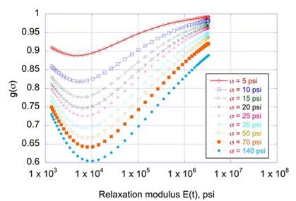
Figure 269. Graph. Variation of g(σ) with stress and E(t) of AC layer.
Subsequently, similar to the k-θ-τ model, the k-θ model was also implemented in the proposed generalized QLV algorithm and was analyzed on a 35-ms haversine load (synthetic FWD pulse load). As shown in table 58, the section properties were kept the same as used for k-θ-τ model. Two HMA mix properties were considered: control and CRTB (for mix properties refer to figure 73). Again stresses at two radial distance r = 0 and 3.5a within the center of the layer (vertically) were used in calculating unbound base modulus value. In the first trial, the modulus value of unbound granular material in LAVA was calculated using stress state at r = 0. In the second trial, the modulus value of unbound granular material in LAVA was calculated using stress state at r = 3.5a.
Figure 270 (top) and figure 271 (top) show the results when r = 0 was used in LAVAN, whereas Figure 270 (bottom) and figure 271 (bottom) show the results when r = 3.5a was used in LAVAN. The difference between the ABAQUS and LAVAN was quantified using the two variables PEpeak and PEavg defined earlier for k-θ-τ model in figure 78 and figure 79, respectively. Because the model integrated both viscoelastic and nonlinear material properties, both peak deflection as well as creeping of deflection should be predicted with accuracy. PEavg was used to examine the model performance in creeping.
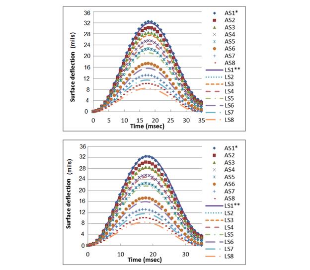
Figure 270. Graphs. Comparison of ABAQUS and LAVAN for nonlinear viscoelastic
structure for the control mix where (top) LAVAN uses stress at r = 0, and (bottom)
LAVAN uses stress at r = 3.5a.
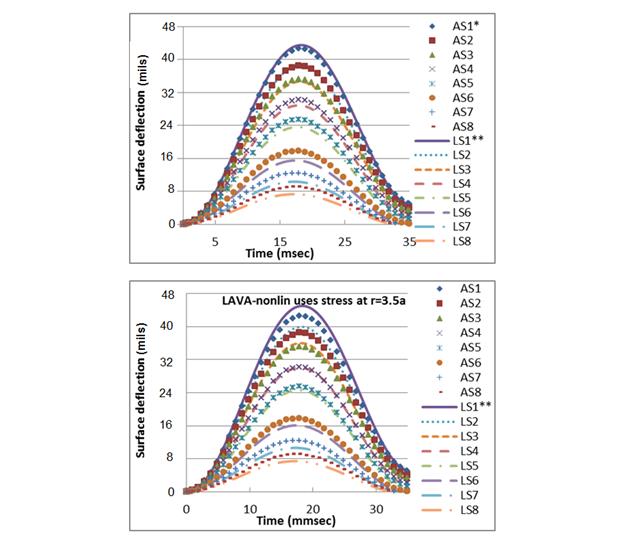
Figure 271. Graphs. Comparison of ABAQUS and LAVA for nonlinear viscoelastic
structure for the CRTB mix where (top) LAVAN uses stress at r = 0 and (bottom) LAVAN
uses stress at r = 3.5a.
As seen in figure 272, slight improvement was observed in PEpeak values for the control mix when stress at r = 3.5a was used to obtain a resilient modulus. However, PEpeak values for CRTB (figure 273) showed a different trend, where first three sensors exhibited lower errors when r = 0 was used. The rest of the sensors did show improvement when r = 3.5a was used. For both the mixes, the creep behavior of the response was well predicted by the model, which can be seen from the low PEavg values in figure 274 and figure 275. However, similar to the k-θ-τ results, r= 0 produced relatively good results, especially in the first four to five sensors.
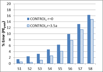
Figure 272. Graph. Percent error (PEpeak) calculated using the peaks of the deflections for
LAVAN-ABAQUS comparison (control mix).
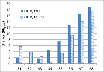
Figure 273. Graph. Percent error (PEpeak) calculated using the peaks of the deflections for
LAVAN-ABAQUS comparison (CRTB mix).

Figure 274. Graph. Average percent error (PEavg) calculated using the entire time history
for LAVAN-ABAQUS comparison (control mix).

Figure 275. Graph. Average percent error (PEavg) calculated using the entire time history
for LAVAN-ABAQUS comparison (CRTB mix).

