U.S. Department of Transportation
Federal Highway Administration
1200 New Jersey Avenue, SE
Washington, DC 20590
202-366-4000
Federal Highway Administration Research and Technology
Coordinating, Developing, and Delivering Highway Transportation Innovations
| REPORT |
| This report is an archived publication and may contain dated technical, contact, and link information |
|
| Publication Number: FHWA-HRT-15-063 Date: March 2017 |
Publication Number: FHWA-HRT-15-063 Date: March 2017 |
This chapter describes the results from a set of experimental procedures designed to evaluate the performance of FWD measurement systems (seismometers, geophones, and accelerometers). Parameters such as accuracy and sensitivity were considered. Observations were used to help test certain features of the numerical tools presented in chapter 5. A high-precision laser system was used in the experimental setups as a reference system and also to evaluate limitations on potential recommendation of its use in FWD systems.
In this section, the research team focused on the key issues to address for potential improvements to FWD testing and interpretation. The identified issues were the following: (1) FWD data collection and measurement; and (2) analysis methods, i.e., static versus dynamic, linear versus nonlinear; and viscoelastic behavior of the AC material. A review of the basic mechanisms and characteristics of the measurement systems available in FWD equipment was conducted.
The research team found that FWD systems available in North America used either geophones or seismometers as sensors to measure the deflection basins. Geophones fell between accelerometers and seismometers in function and price. Seismometers were typically larger and more expensive and usually detected extremely small movements at lower frequencies than geophones. The team learned that some seismometers could be very fragile, and calibrating a seismometer was critical to obtaining useful data. Therefore, a geophone or an accelerometer would more likely be used to get a simpler signal. Because accelerometers are nearly solid state, they are good at handling more violent motion.
Because the measurements are done in a moving reference frame (the pavement surface), almost all sensors are based on the inertia of a suspended mass, which tends to remain stationary in response to external motion. The mass is used as the reference in the system. Therefore, the relative motion of the suspended mass and the ground is a function of the pavement’s motion. Because the sensor is moving with the ground and there is no fixed, undisturbed reference available means that the displacement cannot be measured directly, and according to the inertia principle, one can observe the motion only if it has an acceleration. The frequency response of the mass-spring system is thus a critical factor that greatly influences the sensitivity and the accuracy of the measurement devices.
The basic principle of a geophone involves use of a moving coil within a magnetic field. This can be implemented by having a fixed coil and a magnet that moves with the mass or a fixed magnet and the coil moves with the mass. The output from the coil is proportional to the velocity of the mass relative to the frame. This kind of electromagnetic geophone is called a velocity transducer. Therefore, the measured output from a geophone is related to ground movement through a two-stage transfer function—first a second-order differential transformation describing the mechanical system movement, followed by the electrical system relation obeying the Faraday’s law and describing the generated current in the coil, which is theoretically proportional to velocity. Figure 237 shows an example of the frequency response characteristics for the two stages. Even though the mechanical system exhibited a relatively flat response at low frequencies, the performance of the overall combined response for an in-series configuration fell considerably for low frequencies.

Figure 237. Graphs. Frequency response of geophone components.
For a seismometer, the relative motion of the mass with respect to the casing of the sensor is measured directly using LVDTs. The natural frequency of the mass-spring system and the damping must be tuned to control the sensitivity of the module. The sensitivity (of a seismometer) is defined as the ratio of the maximum motion of the mass to the maximum ground motion during steady-state motion; it is a measure of magnification developed directly at the transducer.
Figure 238 shows the amplitude response of a sensor with a natural period of 1 s and damping ranging from 0.25 to 4 h. As can be seen, low damping resulted in a peak in the response function that occurred for ratio values less than 1. If damping was equal to 1, the seismometer mass returned to its rest position in the least possible time without overshooting, the response curve had no peak, and the seismometer is said to be critically damped. From the shape of the curve, it can be seen that the seismometer could be considered a second-order high pass filter for ground displacement. Seismometers perform optimally at damping close to critical. When the damping increases above 1, the sensitivity decreases and the response approaches that of a velocity sensor.
If the ground displacement frequency were near the resonance frequency, a larger relative motion would be induced (depending on damping). If the damping was low, the mass could get a push at precisely the right time such that the mass would move with a larger and larger amplitude, thus the gain would be larger than 1. For this to occur, the push from the ground would have to occur when the mass was at an extreme position (top or bottom) and there must be a phase shift of - π/2.
Below the resonance frequency, the relative displacement due to ground displacement would decrease. With the ground moving very slowly, the mass would have time to follow the ground motion; in other words, there would be little relative motion and less phase shift. Thus the gain would be low. Therefore, for small frequencies, the relative displacement of the mass would be directly proportional to the ground acceleration. The sensitivity of the sensor to low frequency ground acceleration would be inversely proportional to the squared natural frequency of the sensor.
Strictly speaking, none of the sensors are linear—in the sense that an arbitrary waveform of ground motion can be exactly reproduced at scale—for any kind of response.

Figure 238. Diagram and Graph. A mechanical inertial seismometer with a natural frequency of 1 Hz.
Based on the collected information concerning the frequency behavior of the different measuring devices, a time-frequency analysis was conducted. Measured real field signals were analyzed in the time and frequency domains. The objective was to determine the location, with respect to the signal peak, of frequencies that were artificially filtered by the mechanical spring-mass system, which reduces the accuracy of the sensors (figure 239 through figure 244). The spectrograms, or time-frequency representations of a signal shown in these figures, are 2-D visual representations of the spectrum of frequencies in a signal as they vary with time. The colors illustrate the distribution of the energy contained in the signal as a function of time (x-axis) and frequency (y‑axis). The spectrogram is equivalent to a tracing of the frequency response of the analyzed signal in a moving time window. The unit is the decibel, which is a logarithmic unit commonly used to express the ratio between a reference value and the value of a physical quantity measured in units of power or intensity.
As discussed in the previous paragraph, the different measuring instruments eliminate certain frequencies because of poor performance in some specific ranges. Therefore, it is important to know in what time window (before or after the peak) the eliminated frequencies occur. Also, the comparison between the time-frequency contents of the load and the response from the sensors help in determining the effect of time synchronization.

Figure 239. Graphs. Time-frequency content of the load for LTPP section 60565.

Figure 240. Graphs. Time-frequency content of the load for LTPP section 320101.

Figure 241. Graphs. Time-frequency content of the load for LTPP section 400113.

Figure 242. Graphs. Spectrum of deflection at each sensor for LTPP section 60565.

Figure 243. Graphs. Spectrum of deflection at each sensor for LTPP section 320101.

Figure 244. Graphs. Spectrum of deflection at each sensor for LTPP section 400113.
In light of the literature review of the FWD equipment and the above interpretations, the following issues and observations were identified:
Different sensor types were identified and acquired. A seismometer, a geophone, and an accelerometer were tested. Figure 245 shows the acquired systems. An in-house data acquisition module was built to extract the raw unfiltered data from all the measurement sensors.

Figure 245. Photos. Geophone (left), seismometer (center), and high-accuracy piezoelectric accelerometer (right).
A laser head capable of noncontact measurement of deflections was also tested. Preliminary evaluations of the laser under simulated real field conditions were conducted at the testing facility at FHWA’s Turner-Fairbank Highway Research Center (TFHRC) (see figure 246).

Figure 246. Photos. Setup attached to the FWD system at TFHRC.
The objective was to determine the induced errors (noise) in the recorded signal from the laser in a non-controlled environment. A sample of the obtained signal and its frequency content are shown in figure 247.

Figure 247. Graphs. Sample measured signal (left) and frequency content (right).
The signal-to-noise ratio (SNR) was calculated as 122 for the recording shown in figure 247. This high SNR factor indicated that most of the power in the signal was useful information, and there was very little background noise, which can be identified and filtered. A variation of ±10percent was observed in the calculated ratios for all measured signals. In addition, the accuracy was evaluated to be on the order of 10-5 mil.
The recorded deflection was not compared with the output of the FWD system because of the unavailability of the control laptop computer for the machine during the testing.
To improve the accuracy of the laser measurements, a new more accurate system was acquired. The system and the properties of the new laser head are shown in figure 248. Furthermore, observations during the testing showed that vibrations in the mounting device were a major cause of induced noises. Specific fixtures were built to attach to different models of FWD machines. Figure 249 shows the design for the fixture.

Figure 248. Photos. LK-H008 laser head for deflection measurement.

Figure 249. Diagram. Schematic of the designed fixture.
A set of laboratory tests were conducted to evaluate the performance of the geophone sensor. Two series of tests were conducted: First, the research team placed the geophone directly on the beam and side by side with the laser sensor (see figure 250). Then the geophone was placed in its encasement provided by the manufacturer and situated symmetrically opposite to the laser sensor relative the MTS® load actuator (see figure 251). For this second set of tests, the team also introduced noise on the system by independently vibrating the test setup while placing an accelerometer on the MTS® system so that the noise could be filtered out of the signal.
Figure 252 shows an example of raw velocity signal data from the geophone, and figure 253 shows the filtered velocity data. The figures show that the velocity signal was not symmetrical about zero and that some cyclic behavior occurred post loading time.
Figure 254 shows multiple replications of the laser displacement readings. The data show that the laser was capable of producing a faithful and repeatable deflection signal.

Figure 250. Photo. Geophone placed directly on beam next to laser sensor.
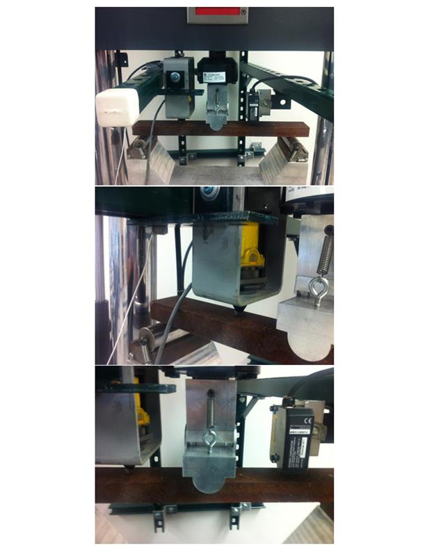
Figure 251. Photos. Test setup for mounted geophone and laser sensor.

Figure 252. Graph. Example of raw data from geophone.

Figure 253. Graph. Filtered geophone data with multiple replications.

Figure 254. Graph. Laser data with multiple replications.
Figure 255 and figure 256 show comparisons between the geophone and laser data for the first test series. When comparing velocity measurements, laser displacement signal was differentiated with respect to time. When comparing deflection measurements, geophone measurements were integrated with respect to time. The measurements showed some significant differences between the two systems, especially after the load returned to zero.
Figure 257 shows similar behavior for the second test series. From the conducted tests, it was clear that numerical errors played a significant role in altering the recorded signals. A set of tests was devised to illustrate the effect of numerical integrations on the collected data to be used in the tools introduced in chapter 5.

Figure 255. Graphs. Comparison of filtered geophone velocity data with the laser derivative output for test series 1.

Figure 256. Graphs. Comparison of integrated geophone data with direct laser displacement output for test series 1.

Figure 257. Graphs. Comparison of integrated geophone data with direct laser displacement output for test series 2.
A series of field tests were performed with the objective of illustrating the effects of drifts and errors induced by numerical integrations and filtering/treatment of raw data collected from inertial sensors (geophones). A KUAB FWD system (owned by the Michigan Department of Transportation (MDOT)), which uses seismometers, was outfitted with a geophone (see figure 258). Loading tests, at four different load levels, were performed on a thin asphalt layer covering a granular structure. Raw data were collected directly from the sensors and compared with the output rendered by the device software (see figure 259).

Figure 258. Photos. Test setup.

Figure 259. Graphs. Sample of recorded raw geophone data.
The use of numerical integration of acceleration or velocity information from inertial sensors to obtain position information inherently causes errors to grow with time, commonly known as “integration drift.” The main problem is that integrating a signal contaminated with noise and drift leads to an output that has an RMS value that increases with integration time even in the absence of any motion of the sensor. For a single integration, the errors are a function of the duration of the signal. For that reason, estimation of deflections using inertial sensors is usually performed with the help of externally reference-aided sensors or sensing systems, or prior knowledge about the motion to correct for the drift. With aided sensors or sensing systems, KFs or EKFs are commonly used to fuse different sources of information in an attempt to correct for the drift.
For real-time compensation, zero-phase adaptive filtering algorithms are employed. These algorithms are based on truncated Fourier series such as weighted-frequency Fourier linear combiner (WFLC) or band-limited multiple Fourier linear combiners (BMFLCs), which can detect periodic or quasi-periodic signals. These algorithms can estimate desired periodic signals from a mixture of desired periodic signals and undesired signals without altering the phase and magnitude of the desired periodic signal. However, to achieve satisfactory accuracy of the estimate, the WFLC and the BMFLC have limitations—the magnitude of the undesired signals compared with that of the desired periodic signal cannot be too large. Because the magnitude of the integration drift is too large compared with that of the periodic signal, the algorithms are not well suited for the problem of drift.
For the tests performed, the research team needed to obtain drift-free deflection estimates of the quasi-periodic motion using the geophone sensor without employing other aided sensors or sensing systems. An example of the effects induced by the numerical integration is shown in figure 260. The methods used to obtain the test results are based on linear high-pass filtering of drifted position by selecting a cutoff frequency between the frequencies of low-frequency drift signals and that of the periodic motion, which had relatively high frequency (the effect of the cutoff frequency selection is shown in figure 261). A specific cutoff frequency was selected for each dataset. Optimal values were used to obtain the final result shown in figure 262 and figure 263. One of the issues observed was that linear filtering inherently introduced phase shift and attenuation, resulting in inaccurate deflection-amplitude estimates. A combination of linear filtering and WFLC was used. The integrated signal was filtered using a high-pass linear filter. The filtered signal, which was the phase-shifted and amplitude-modified version of the actual desired signal, was then estimated using WFLC algorithms. The estimate of the actual periodic signal was recovered from the phase-shifted and modified estimate by compensating for the phase-shift and amplitude alteration introduced by the filter.

Figure 260. Graph. Example of numerical drift resulting from integration of raw geophone data.

Figure 261. Graphs. Illustration of the windowing and filtering procedure and the observed
effects on the raw velocity data: frequency content of the velocity signal (left) and effect of
the selected cutoff frequency on the signal magnitude as a source of errors (right).
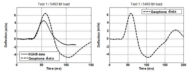
Figure 262. Graphs. Comparison between the filtered and treated seismometer data
rendered by the device software and the integrated unfiltered geophone data (left); and
integrated and filtered geophone data showing post-peak effects due to propagation of
cumulative errors (right).

Figure 263. Graphs. Comparison between the filtered and treated seismometer data
rendered by the device software and the integrated unfiltered geophone data at different
load levels.
The FWD system (owned by the MDOT), which uses seismometers, was outfitted with a laser for direct deflection measurements. Loading tests, at four different load levels, were performed on a section of a local road. Raw data were collected directly from the laser and compared with the output rendered by the commercial software used.
The laser was mounted on a beam that was attached to the ground on the roadside (see figure 264). The objective was to isolate the beam from the effects of the vibrations in the pavement.
Given the high accuracy of the laser system, even small vibrations are picked up in the signal. For the tests performed, a poor SNR was observed. The measurements from the laser had to be filtered and adjusted. An example is shown in figure 265.
As figure 265 shows, the post peak fluctuations rendered in the laser signal were not included in the KUAB signal, which was cut off at 120 ms. More important, the difference in deflection time histories seemed to be much larger in the post peak region. This would seem to confirm anecdotal assertions made by FWD specialists over the years.

Figure 264. Photos. FWD test setup: view of the beam used for mounting the laser (top left),
close-up view of mounted laser (top right), and view of laser sensor setup (bottom).

Figure 265. Graph. Comparison between the seismometer data rendered by the KUAB
software and the filtered and treated laser data measured for a 9,500-lbf load.
This chapter describes a set of experimental procedures conducted both in the laboratory and in the field using seismometers, geophones, and accelerometers. The experiments were designed to evaluate the performance of the sensors in term of accuracy and sensitivity, with the objective of including the effects of these parameters in the tools described in previous chapters.
Based on the observations, the following issues were discussed:
In addition, a study was presented to illustrate the effects of numerical integrations and drifts, confirming their significant influence on the output results.
For all the tests presented, a high-precision laser system was used in the experimental setups as a reference system and also to evaluate limitations on potential recommendation of its use in FWD systems. Even though the laser system performed flawlessly under laboratory conditions and was successfully used as a reference for characterizing the other devices, it was much more difficult to use in the field. Given the high accuracy of the laser, even small vibrations were picked up in the signal. Therefore, field measurements from the laser also had to be filtered and adjusted. The advantages of using a laser were mainly that it eliminated all the undesirable effects from numerical artifacts because it directly measured the deflection. This is similar to seismometers but with the added advantage that it was a noncontact method so there were no seating errors. The main disadvantage was that lasers still need a fixed reference in the system to extract the pavement’s true surface motion. This could be achieved by either disconnecting the rigid bar that holds the sensors away from the FWD machine frame, thus isolating the frame from the vibration noise, or by placing an external reference mechanism away from the influence of the deflection basin induced by the load drop. The external reference could be position sensors that track the movement of the beam holding the sensors. This was previously done using accelerometers but would not solve the problem because it would require a double integration for the accelerometer data.
Geophones have the advantage of not requiring an added reference, but it was shown in the studies reported in this chapter that data were relatively less reliable post-peak. Geophones are based on the inertia of a suspended mass, which means they have performance issues at low frequencies. Furthermore, the requirement for a numerical integration induces several numerical artifacts such as errors in post-peak amplitude and drifts.
The issue with time synchronization between the load and the measurements output was an easy technological fix. The focus of existing FWD systems has been to determine the response peaks, which are not affected by the synchronization problem. This becomes important when the whole time response is of interest. This issue could be resolved by adding a position sensor that records the exact position of the dropping mass. The position sensor should be connected to the same data acquisition system as all the sensors so that it uses the same timer.

