Enhanced Analysis of Falling Weight Deflectometer Data for Use With Mechanistic-Empirical Flexible Pavement Design and Analysis and Recommendations for Improvements to Falling Weight Deflectometers

APPENDIX B. THEORETICAL ANALYSES ON MULTIPLE-PULSE FWD'S IN BACKCALCULATION

As discussed in chapter 4, responses of viscoelastic materials show dependence on time (or frequency), rate of loading, and temperature. The relationship of characteristic viscoelastic properties such as relaxation modulus, creep compliance, and dynamic modulus with time (or frequency) are often expressed at a specific reference temperature, in terms of a master curve. In theory, it should be possible to obtain such a curve if data containing time-changing responses at different temperature levels are known. The available analysis window for the current FWD devices is short, extending up to 25 to 35 ms of stress pulse. However, the recorded information can be used to infer part of the relaxation function. As for temperature information, it is possible to test the same location at different times within a day. Although a series of FWD tests at different temperatures could be useful in developing the entire master curve, in theory the prediction can be improved if information at different rates of loading or over a larger time interval were known. In this appendix, these possibilities are explored. Note that backcalculation in this appendix was performed using the MATLAB® optimization function fminsearch.

BACKCALCULATION USING MULTIPLE PULSES AT DIFFERENT FREQUENCIES

To illustrate the possibility of exploiting information from multiple frequencies in backcalculation of the damaged HMA master curve, two examples are presented. In the first, a typical FWD pulse was backcalculated, and in the second example, multiple FWD pulses at different frequencies were backcalculated. For these two examples, forward computations were performed using a known E(t) to compute the deflection basin. Figure 276 shows the E(t) master curve that was used in these examples. For simplicity, the AC layer temperature was assumed to be equal to the reference temperature of the master curve (T_ref = 66.2 °F); therefore, t_R= t = actual time.

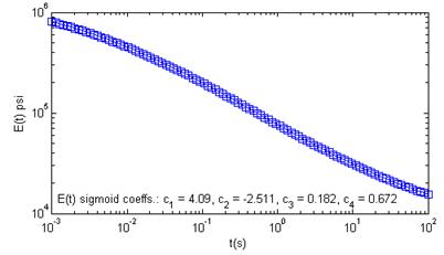
Figure 276. Graph. E(t) used to compute the deflection basin in examples 1 and 2.

Example 1–Typical FWD Pulse

In this example, to simulate a typical FWD pulse, a haversine loading with a duration of 35 ms, followed by a rest period of 35 ms, was simulated (figure 277 (left)). Figure 277 (right) shows the resulting deflection basin at different radial distances from the centerline of the load.

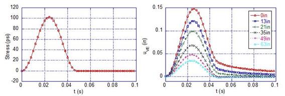
Figure 277. Graphs. FWD deflection history for example 1.

In this example, the only unknown parameter was the E(t) master curve of the AC layer. Other parameters, such as unbound layer modulus, Poisson’s ratio, and thicknesses of AC and unbound layers, were known. In addition, a constant Poisson’s ratio of 0.35 was assumed for the AC layer. Initially, a random number generator was used to determine the initial sigmoid constants. Figure 278 (left) shows the initial sigmoid coefficients and the resulting initial E(t) curve, which was quite different from the actual E(t) curve. Such an initial difference was important to ensure that the backcalculation procedure worked accurately without depending on the initial values. Backcalculation results at the starting and the ending stage of optimization are shown as continuous line in the figure. Figure 278 (right) shows the final backcalculation results obtained at the end of the optimization, where a very good agreement was observed. Figure 279 shows the backcalculated |E*| and Φ values, along with the actual values. Consistent with E(t), a good match between the backcalculated and actual values was obtained at frequencies higher than 10^-3 Hz in both |E*| and Φ. However, curves diverged at lower frequencies. This was not unexpected because only the early portion of the E(t) curve was used in calculation of deflection history shown in figure 276. Later portions of the E(t) curve (and |E*| and Φ values at low frequencies) can be obtained by increasing the pulse duration or using a different form of stress history, which is shown in the next example.

Figure 278. Graphs. E(t) and deflection history at the initial (left) and final (right) backcalculation stage in example 1.

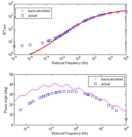
Figure 279. Graphs. Comparison of backcalculated and actual |E*| and phase angle master curves for example 1

Example 2–Cyclic Pulses With Two Different Frequencies

In this example, four successive pulses with durations of 35 ms, followed by four pulses with 10s durations, were simulated to generate the deflection basin (figure 280). This example was used to investigate whether a different loading history could result in better estimation of E(t). Figure 281 shows the backcalculated E(t), where a much better fit can be seen. Note that the accuracy of the backcalculated E(t) depended on the duration of the stress pulse, where longer duration allowed calculation of E(t) at longer durations. It was also important to apply high-frequency (short duration) pulse load to increase the accuracy of E(t) at very short times. Backcalculation of E(t) for this example took less than 5 min. Figure 282 shows the backcalculated |E*| and phase angle master curves, where a much better match can be seen compared with example 1.

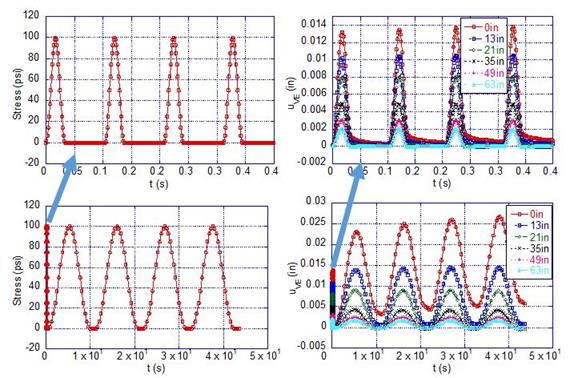
Figure 280. Graphs. Applied stress and resulting deflection basin for example 2.

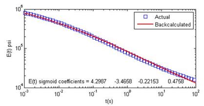
Figure 281. Graph. Backcalculated E(t) using multiple stress pulses.

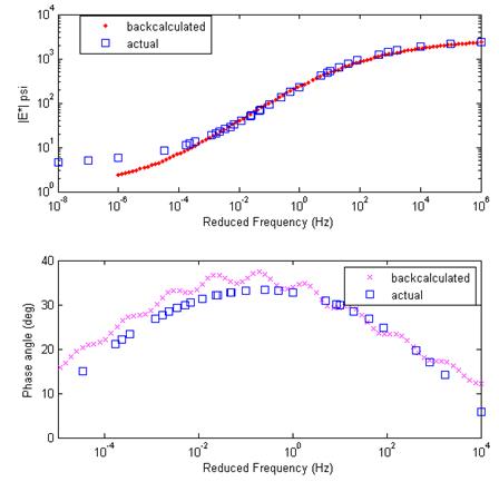
Figure 282. Graphs. Comparison of backcalculated and actual |E*| and master curves for example 2.

BACKCALCULATION USING SERIES OF MULTIPLE-PULSE FWDS AT CONSTANT FREQUENCY AND DIFFERENT TEMPERATURE

The theoretical FWD stress history shown in figure 283 was used to investigate whether a loading history with multiple pulses at constant frequency could improve the backcalculation results. First, deflection time histories were computed at several temperatures using LAVA. Then, BACKLAVA was used to backcalculate the E(t) master curve. Two examples are shown. In the first, three successive pulses with durations of 80 ms, followed by a rest period of 760ms, were simulated to generate deflections. In the second, only the initial three successive pulses were used, and deflection over the remainder of the period was ignored.

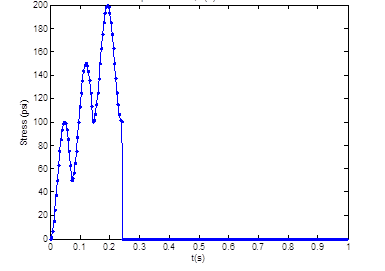
Figure 283. Graph. Stress history used in the constant frequency multiple pulse analysis.

Example 1

The LAVA algorithm was used to compute deflection histories resulting from the loading shown in figure 283 at the temperatures 50, 86, 104, 140, 176, 212, and 248 °F. Measured and backcalculated responses for temperatures 50, 86, 104, and 140 °F are shown in figure 284. The backcalculated E(t) curve after 1 h 7 min is shown in figure 285. The results obtained for the backcalculation using multiple pulses were encouraging because of the increased time and relaxation due to the stress history.

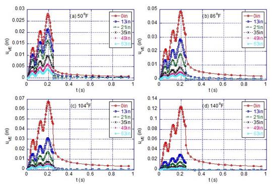
Figure 284. Graphs. Deflection at different sensors at different temperatures in example 1.

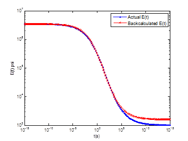
Figure 285. Graph. Result for backcalculated E(t) curve in example 1.

Example 2

In example 2, the problem was solved only for the pulse duration; the relaxation trend was omitted. The problem was solved for a temperature set of 32, 50, 68, 86, 104, 122, 140, 158, 176, 194, 212, 230, and 248 °F. The backcalculated E(t) values for example 2 at 1 h 7 min are plotted in figure 286. Measured and backcalculated deflection histories for temperature 32, 50, 68, and 86°F are shown in figure 287.

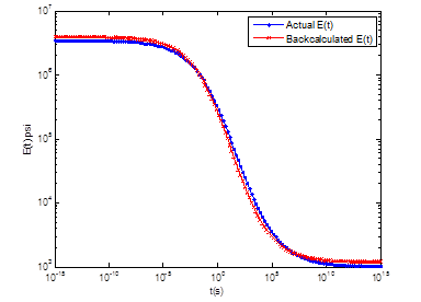
Figure 286. Graph. Result for backcalculated E(t) curve for example 2.

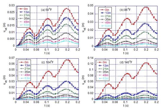
Figure 287. Graphs. Deflections at different sensors at different temperatures for example 2.

Note that the accuracy of the backcalculated E(t) curve depended on the duration and temperature of the stress pulse loading. Inclusion of high temperatures along with an elongated stress pulse in the theoretical analysis allowed calculation of E(t) at longer durations. It can be seen from figure 285 and figure 286 that the backcalculated E(t) curve obtained from using both truncated and nontruncated deflection curves showed good prediction. However, a much more accurate predicted E(t) curve up to 10⁵ s was obtained when nontruncated deflection curves were used in backcalculation.

CONCLUSIONS

The results from the four examples presented in this appendix suggest that including FWD pulses or multiple frequencies in backcalculation may improve the accuracy of the E(t) master curve prediction. The improvement in backcalculated E(t) master curve could be for two possible reasons—an increase in the deflection time history and a different rate of loading. However, more comprehensive theoretical analyses are needed to assert and determine the optimal loading history that should be applied by an FWD. Although the theoretical methods suggested in this appendix clearly have potential to improve the ability of BACKLAVA in predicting E(t) master curve, the methods have the following limitations:

• Increasing the number of FWD pulses (i.e., the frequency content) increases the computational time of the backcalculation, making it computationally expensive.
  
  
• Different frequencies in the loading history alone cannot be used to obtain both the time and temperature properties of the HMA layer, which are needed for complete characterization of the HMA layer.