U.S. Department of Transportation
Federal Highway Administration
1200 New Jersey Avenue, SE
Washington, DC 20590
202-366-4000
Federal Highway Administration Research and Technology
Coordinating, Developing, and Delivering Highway Transportation Innovations
| REPORT |
| This report is an archived publication and may contain dated technical, contact, and link information |
|
| Publication Number: FHWA-HRT-15-063 Date: March 2017 |
Publication Number: FHWA-HRT-15-063 Date: March 2017 |
Flexible pavements are multilayered structures typically with viscoelastic AC as the top layer and with unbound/bound granular layers below it. The combined response of linear viscoelastic and elastic materials that are in perfect bonding is linear viscoelastic. Assuming there is full bonding between the asphalt layer and the underlying base and subgrade layers, the overall response of the entire pavement system becomes viscoelastic. The characteristic mechanistic properties of an isotropic-thermorheologically simple viscoelastic systems are the relaxation modulus E(t), the creep compliance D(t), the complex (dynamic) modulus |E*|, and the time-temperature shift factors (aT(T)). These characteristic properties are often expressed at a specific reference temperature, in terms of a “master curve.” For thermorheologically simple materials, these characteristic properties can be generated at any time (or frequency) and temperature using the time-temperature superposition principle. It can be shown that if any of the three properties E(t), D(t), or |E*| is known, the other two can be obtained through an interconversion method such as the Prony series.(57) The dynamic modulus (|E*|) master curve of an AC layer is a fundamental material property that is required as an input in the MEPDG for a flexible pavement analysis. Knowledge of the |E*| master curve of an in-service pavement using FWD data can lead to a more accurate estimation of its remaining life and rehabilitation design.
The specific objectives of this component of the project were to (1) develop a layered viscoelastic flexible pavement response model in the time domain; (2) investigate whether the current FWD testing protocol generated data that were sufficient to backcalculate the |E*| master curve using such a model; and (3) if needed, recommend enhancements to the FWD testing protocol to be able to accurately backcalculate the |E*| master curve as well as the unbound material properties of in-service pavements. Readers should note that the methods presented in this report were developed for a single AC layer. However, in-service pavements may be composed of multiple layers of different types of asphalt mixtures. In such cases, the present form of the backcalculation algorithms would provide a single equivalent |E*| master curve for the asphalt mixture sublayers.
The models presented in this chapter can consider the unbound granular material as both linear elastic as well as nonlinear stress-dependent material. Depending on the assumed unbound granular material property, two generalized viscoelastic flexible pavement models were developed. The developed forward and backcalculation models for linear viscoelastic AC and elastic unbound layers are referred to as LAVA and BACKLAVA, respectively, in this report. The developed forward and backcalculation models for linear viscoelastic AC and nonlinear elastic unbound layers are termed LAVAN and BACKLAVAN, respectively, in the report. The LAVA and BACKLAVA algorithms assumed a constant temperature along the depth of the AC layer. The algorithms were subsequently modified for the temperature profile in the AC layer, and modified versions are referred to as LAVAP and BACKLAVAP in this report. The viscoelastic properties backcalculated from FWD data included two functions—a time function and a temperature function. The time function referred to the relaxation modulus master curve E(t,T0) in which t was physical time and T0 was the corresponding (constant) reference temperature. The temperature function referred to the time-temperature shift factor aT(T), which was a positive definite dimensionless scalar. In the present study, AC was assumed to be thermorheologically simple, which allowed applying E(t,T0) for any temperature level T (different than T0) by simply replacing physical time with a reduced time tR = t/aT(T); therefore, aT(T) is a function of both T and T0, such that aT(T)=1 if T = T0.
Typically, a load-displacement history of 60 ms is recorded in an FWD test (which constitutes 25to 35 ms of applied load pulse); it is generally observed that the later portion of deflection history (after the peak) is not reliable. This is due to the numerical error generated by velocity integration. (Most FWD sensors measure velocity or acceleration, which is integrated to obtain the deflections.) This can give only limited information about the time-varying E(t) behavior of the AC layer. However, in theory, it should be possible to obtain the two sought-after functions (i.e., E(t) and aT(T)). In this report, two different approaches are discussed to obtain the comprehensive behavior of asphalt: (1) using series of FWD deflection time histories at different temperature levels and (2) using uneven temperature profile information existing across the thickness of the asphaltic layer during a single or multiple FWD drops deflection histories.(59,60) Both of the models are presented in detail. Finally, the models were validated using frequency and FEM-based solutions.
Further, the effect of FWD test temperatures and number of surface deflection sensors on backcalculation of the |E*| master curve were studied. These suitable FWD test data requirements are discussed in the key findings from the study.
Traditionally, flexible pavements are analyzed using analytic multilayered elastic models (e.g., KENLAYER, BISAR, and CHEVRONX), which are based on Burmister’s elastic solution of multilayered structures. (See references 21, 23, 27, and 61–64.) These models assume the material in each pavement layer is linearly elastic. However, the AC (typically the top layer) is viscoelastic at low strain.(60,65,66) As with any viscoelastic material, it shows properties dependent on time (or frequency) as well as temperature.
In the proposed approach, the AC pavement system was modeled as a layered half-space, with the top layer as a linear viscoelastic solid. All other layers (base, subbase, subgrade, and bedrock) in the pavement were assumed linear elastic. Assuming there was full bonding between the AC layer and the underlying base and subgrade layers, the overall response of the entire pavement system became viscoelastic. Therefore, its response under arbitrary loading was obtained using Boltzmann’s superposition principle (i.e., the convolution integral) as shown in figure 26.(65,66)

Figure 26. Equation. Boltzmann’s superposition principle.
Where:
Rve(x, y, z, t) I = the linear viscoelastic response at coordinates (x,y,z) and time t.
RHve (x, y, z, t) = the (unit) viscoelastic response of the pavement system to a Heaviside step function input (H(t)).
dI(τ) is the change in input at time τ.
It is worth noting that for a uniaxial viscoelastic system (e.g., a cylindrical AC mixture), if response Rve= ε (t) = strain, then RHve = D(t) = creep compliance and I(t) = σ(t) = stress. Using Schapery’s quasi-elastic theory, the viscoelastic response at time t to a unit input function was efficiently and accurately approximated by the elastic response obtained using relaxation modulus at time t as shown in figure 27.(67,68)
![]()
Figure 27. Equation. Quasi-elastic approximation of a unit response function such as the creep compliance.
Where RHe(x,y,z, E(t)) is the unit elastic response at elastic modulus equal to relaxed modulus (E(t)). Flexible pavements are exposed to different temperatures over time, which in turn influence their response. For thermorheologically simple materials, this variation in response can be predicted by extending the equations shown in figure 26 and figure 27 to the equation shown in figure 28.

Figure 28. Equation. Hereditary integral using quasi-elastic approximation of a unit response function such as the creep compliance.
Where:
tR = t/aT(T).
aT (T) = a1 (T2- T2ref ) + a2 (T - Tref ) is the shift factor at temperature T.
Tref I = the reference temperature
a1 and a2 are the shift factor’s polynomial coefficients.
Using figure 28, the formulation for predicting vertical deflection of a linear viscoelastic AC pavement system subjected to an axisymmetric loading can be expressed as the equation shown in figure 29.
![]()
Figure 29. Equation. Hereditary integral using quasi-elastic approximation of unit vertical deflection at the surface.
Where:
uvevertical (r,z,t) = the viscoelastic response of the viscoelastic multilayered structure at time t and coordinates (r,z).
ueH -vertical (E(tr - τ ),r,z ) i = the elastic unit response of the pavement system at reduced time tR due to the unit (Heaviside step) contact stress (i.e., σ (t )= 1).
σ (τ) is the applied stress at the pavement surface.
Detailed derivation of the equation in figure 29 can be found in Levenberg’s research and are not repeated here for brevity.(69) In this implementation, the vertical surface displacements, i.e., uveH (t) ≅ ueH (t) values at the points of interest, were computed using the CHEVRONX layered elastic analysis program. Then the convolution integral in figure 29 was used to calculate the viscoelastic deflection uve(t). A description of the algorithm is given in the following section.
The algorithm steps were as follows:

Figure 30. Diagram. Typical flexible pavement geometry for analysis.

Figure 31. Graph. Discretization of stress history in forward analysis.
![]()
Figure 32. Equation. Sigmoid form of relaxation modulus master curve.
Where tR is the reduced time (tR = t/aT(T)) and ci are sigmoid coefficients. The shift factor coefficients were computed using the second order polynomial given in figure 33.
![]()
Figure 33. Equation. Shift factor coefficient polynomial.
Where a1 and a2 are the shift factor coefficients.

Figure 34. Graph. Discretization of the relaxation modulus master curve.
![]()
Figure 35. Equation. Quasi-elastic approximation of unit vertical deflection at the surface.
The equation in figure 35 is calculated using E(ti) where i = 1,2,3…NE. Figure 36 shows the ueH values calculated for points at different distances from the centerline of the circular load at the surface. These curves are called unit response master curves.

Figure 36. Graph. Deflections calculated under unit stress for points at different distances from the centerline of the circular load at the surface.
![]()
Figure 37. Equation. Discrete formulation.
Where I = 1,2,…Ns.

Figure 38. Graph. dσ( τj ) for each time step τj
To illustrate an example, the viscoelastic surface deflections of the three-layer pavement structure shown in figure 39 were computed. Figure 40 shows the vertical surface deflections at points located at different radial distances from the centerline of the load. Figure 40 clearly shows the relaxation behavior of deflection at each point.

Figure 39. Diagram. Example problem geometry.

Figure 40. Graph. Examples of computed viscoelastic surface deflections at different radial distances from the centerline of the load.
One of the primary reasons for implementing Schapery’s quasi-elastic solution is its extreme computational efficiency. Using a Pentium 2.66 GHz computer with 3.25 gigabytes (GB) of random access memory (RAM), the computation of the results shown in figure 40 took 1.96 s to calculate the solution for the three-layer system shown in figure 39 and NS = 50, NE = 50.
Table 10 shows the computation times for different numbers of discrete time steps in the three-layer system.
Table 10. LAVA computation times for different numbers of discrete time steps.
| NS | NE | Computation Time (s) |
|---|---|---|
| 50 | 50 | 1.96 |
| 24 | 100 | 2.88 |
| 50 | 100 | 3.03 |
| 100 | 100 | 3.05 |
| 100 | 200 | 5.01 |
| 200 | 200 | 5.13 |
The layered viscoelastic algorithm was verified by using two pavement structures selected from the SPS‑1 experiment of the LTPP database (table 11). Surface deflections at different radial distances due to a circular loading pulse of 0.045 s followed by 0.055-s rest period were calculated using two commonly known software packages, SAPSI and LAMDA, and compared with the layered viscoelastic solution implemented in this research. SAPSI is based on damped-elastic layer theory and FEM, whereas LAMDA is based on the spectral element technique, axisymmetric dynamic solution.(32,2) These software packages were selected because they were known to provide robust dynamic solutions, and their algorithms were based on frequency-domain calculations. This allows truly independent verification because the layered viscoelastic solution is in the time domain, whereas SAPSI and LAMDA are in the frequency domain.
Table 11. Pavement properties used in LAVA validation with SAPSI and LAMDA.
| Case No. | Physical Layer | Elastic Modulus | Thickness (inches) |
Poisson’s Ratio |
|---|---|---|---|---|
| 116 | AC | |E*|-fro | 3.9 | 0.35 |
| TB base | 29 ksi | 12.0 | 0.40 | |
| Subgrade (SS) | 14.5 ksi | Infinity | 0.45 | |
| 120 | AC | |E*|-fro | 3.6 | 0.35 |
| PATB base | 26.1 ksi | 4 | 0.40 | |
| GB base | 21.8 ksi | 8 | 0.40 | |
| Subgrade (SS) | 14.5 ksi | Infinity | 0.45 | |
| TB = Treated base. SS = Sandy subgrade. PATB = Permeable asphalt treated base. GB = Granular base. |
||||
Figure 41 and figure 42 show the comparison between the layered viscoelastic solution and solutions calculated with SAPSI and LAMDA. The figures clearly show that the layered viscoelastic result matched very well to the SAPSI and LAMDA solutions. Note that the layered viscoelastic algorithm did not consider the dynamics, whereas SAPSI and LAMDA did.
The dynamic solution developed a time delay in response to wave propagation. However, because the scope of this portion of the project included the backcalculation of viscoelastic characteristics of the AC layer, the effect of dynamics was not considered. Therefore, the time delay in dynamic solutions was eliminated by shifting the deflection curves to the left such that the beginning of each sensor response matched.

VE = viscoelastic.
41. Graphs. Comparison of dynamic solutions (time delay removed) and viscoelastic solution for case 116.

VE = viscoelastic.
Figure 42. Graphs. Comparison of dynamic solutions (time delay removed) and viscoelastic solution for case 120.
Temperature in pavements typically varies with depth, which affects the response of the HMA to the applied load. As shown in figure 43, the temperature may increase with depth (profile 1—linear, 2—piecewise, and profile 3—nonlinear) or decreasing with depth (profile 4—linear, profile 5—piecewise, and profile 6—nonlinear) depending on the time of the day. This variation in temperature with depth can be approximated with a piecewise continuous temperature profile function as shown in figure 43 (profiles 2 and 5). The advantage of using a piecewise function is that it can be used to approximate any arbitrary function.

Figure 43. Diagram. Schematic of temperature profile.
An algorithm that considers HMA sublayers with different temperatures within the HMA layer was developed and is referred to as LAVAP (T-profile LAVA). The algorithm was compared with LAVA as well as ABAQUS. Comparison with LAVA was made for deflection response at all the sensors for constant temperature throughout all the sublayers. The pavement section and layer properties used in the forward analysis are shown in table 12. Figure 44 shows the response obtained from the temperature profile algorithm at 32, 86, and 122 °F matched very well with LAVA.
Table 12. Pavement properties used in (T-profile LAVA) LAVAP validation with ABAQUS.
| Property | Constant Temperature | Temperature Profile (Three-Step Function) |
|
|---|---|---|---|
| Thickness (inches) |
AC sublayers | 6 | 2, 2, 2 |
| Granular layers | 20, infinite | 20, infinite | |
| Poisson ratio {layer 1, 2, 3…} | 0.35, 0.3, 0.45 | 0.35, 0.3, 0.45 | |
| Eunbound{layer 2, 3…}, psi | 11,450, 15,000 | 11,450, 15,000 | |
| Total number of sensors | 8 | ||
| Sensor spacing from the center of load (inches) | 0, 7.99, 12.01, 17.99, 24.02, 35.98, 47.99, 60 | ||
| E(t) sigmoid coefficient {AC} | 0.841, 3.54, 0.86, -0.515 | 0.841, 3.54, 0.86, -0.515 | |
| a(T) shift factor polynomial coefficients {AC} |
4.42E-04, -1.32E-01 | 4.42E-04, -1.32E-01 | |

Figure 44. Graphs. Comparison of response calculated using (T-profile LAVA) LAVAP and original LAVA.
To qualitatively examine the response of flexible pavement predicted using the (T-profile LAVA) LAVAP algorithm, the response obtained under temperature profile was compared with the response obtained under constant temperatures. As an example, a comparison of the response under a temperature profile of {104, 86, 68} °F, with that corresponding to a constant temperature of 104, 86, and 68 °F for the entire depth, is shown in figure 45, figure 46, and figure 47, respectively. It can be seen from the figures that the effect of AC temperature was most prominent in sensors closer to the load center (sensors 1 through 4). For sensors away from the loading center (sensors 5, 6, 7, and 8), the deflection histories were not influenced by the AC temperature. Figure 48 shows the region of the E(t) master curve (at 66.2 °F reference temperature) used by the (T-profile LAVA) LAVAP algorithm in calculating time histories.

Figure 45. Graph. Comparison of responses calculated using (T-profile LAVA) LAVAP at
temperature profile {104, 86, 68} °F and original LAVA at constant 104 °F temperature.

Figure 46. Graph. Comparison of responses calculated using (T-profile LAVA) LAVAP at
temperature profile {104, 86, 68} °F and original LAVA at a constant temperature of 86 °F.

Figure 47. Graph. Comparison of responses calculated using (T-profile LAVA) LAVAP at
temperature profile {104, 86, 68} °F and original LAVA at a constant temperature of 68 °F.

Figure 48. Graph. Region of E(t) master curve (at 66.2 °F reference temperature) used by
(T-profile LAVA) LAVAP for calculating response at temperature profile {104, 86, 68} °F .
As expected, for a condition of higher temperature at the top and lower temperature at the bottom, the response with a higher constant temperature was always greater than the response with a temperature profile. The response with a lower constant temperature was always less than the response with a temperature profile. The response with a medium constant temperature may or may not be less than the profile response, depending on the temperature profile and thickness of the sublayering.
Next, the LAVA algorithm was validated against a well-known FEM software, ABAQUS, where the temperature profile in the AC layer was simulated as two sublayers of AC with different temperatures. For this purpose, two different HMA types were considered, Terpolymer and SBS64-40. The viscoelastic properties of these two mixes are shown in figure 49. As shown in table 13, for both mixes, the AC layer was divided into two sublayers, with temperature in the top and bottom sublayer assumed to be 66 and 86 °F, respectively.

Figure 49. Graphs. Relaxation modulus and shift factor master curves at a reference temperature of 66 °F.
Table 13. Pavement section used in (T-profile LAVA) LAVAP validation.
| Layer | Modulus (E(t) or E) | Thickness (inches) (Temperature °F) |
Poisson’s Ratio |
|---|---|---|---|
| AC | Mix 1: Terpolymer (E(t) see figure 49) Mix 2: SBS 64-40 (E(t) see figure 49) |
Sublayer1 = 3.94 inches (66 °F) Sublayer2 = 3.94 inches (86 °F) |
0.45 |
| Base | 15,000 psi (linear elastic) | 7.88 inches | 0.35 |
| Subgrade | 10,000 psi (linear elastic) | Infinity | 0.45 |
Figure 50 and figure 51 show a comparison of surface deflection time histories measured at radial distances of 0, 7.99, 12.01, 17.99, 24.02, 35.98, 47.99, and 60 inches for mixes 1 and 2. From the figures, it can be observed that the results obtained from LAVAP and ABAQUS matched well.

Figure 50. Graph. Comparison between LAVAP and ABAQUS at a temperature profile of {66, 86} °F (terpolymer).

Figure 51. Graph. Comparison between LAVAP and ABAQUS at a temperature profile of {66, 86} °F (SBS 64-40).
As expected, it can be seen from table 14 that for both mixes, surface deflection in the pavement section at the two-step AC temperature profile of {66, 86} °F was between the deflections obtained for constant AC temperatures of 66 and 86 °F.
Table 14. Peak deflections at temperature profile {66, 86}°F and at a constant temperature of 86 °F using LAVA.
| Mix | Temperature (°F) | Sensor Deflection (mil) | |||||||
|---|---|---|---|---|---|---|---|---|---|
| 1 | 2 | 3 | 4 | 5 | 6 | 7 | 8 | ||
| Terpolymer | Constant: 66 | 28.1 | 24.7 | 22.5 | 19.5 | 16.8 | 12.4 | 9.3 | 7.2 |
| Profile: 66, 86 | 33.0 | 28.1 | 24.9 | 20.7 | 17.3 | 12.2 | 9.1 | 7.0 | |
| Constant 86 | 38.4 | 30.9 | 26.8 | 21.8 | 17.8 | 12.2 | 8.9 | 6.9 | |
| SBS 64-40 | Constant 66 | 35.2 | 29.1 | 25.7 | 21.3 | 17.6 | 12.3 | 9.1 | 7.0 |
| Profile: 66, 86 | 40.9 | 32.5 | 27.7 | 22.0 | 17.7 | 12.0 | 8.8 | 6.9 | |
| Constant 86 | 47.6 | 35.1 | 29.2 | 22.7 | 17.9 | 12.0 | 8.7 | 6.8 | |
This section presents a computationally efficient layered viscoelastic nonlinear model called LAVAN. LAVAN can consider linear viscoelasticity of AC layers as well as the stress-dependent modulus of granular layers. The formulation was inspired by quasilinear-viscoelastic (QLV) constitutive modeling, which is often used in analyzing nonlinear viscoelastic materials. In the literature, the various forms of the model are also called Fung’s model, Schapery’s nonlinearity model, and modified Boltzmann’s superposition. (See references 70–75.)
LAVAN combines Schapery’s quasi-elastic theory with generalized QLV theory to predict the response of multilayered viscoelastic nonlinear flexible pavement structures. Before introducing the generalized QLV model, a brief overview of granular nonlinear pavement models is presented. This is followed by development of a generalized QLV model for a multilayered system and numerical validation in which the response of flexible pavements under the FWD test was analyzed. The model was validated against the general-purpose FEM software, ABAQUS.
Under constant amplitude cyclic loading, granular unbound materials exhibit plastic deformation during the initial cycles. As the number of load cycles increases, plastic deformation ceases to occur, and the response becomes elastic in further load cycles. Often, elastic response in a triaxial cyclic loading is defined by resilient modulus (MR) at that load level, which is expressed as shown in figure 52.
![]()
Figure 52. Equation. Resilient modulus.
Where:
σd = ( σ1 – σ3), is the deviatoric stress in a triaxial test.
εr = recoverable strain.
If the granular layer reaches this steady state under repeated vehicular loading, then further response can be considered recoverable, and figure 52 can be used to characterize the material. The MR value shown in figure 52 is affected by the stress state (or load level). Typically, unbound granular materials exhibit stress hardening, i.e., MR increases with increasing stress.(76,77) As shown in figure 53, Hicks and Monismith related bulk stress and the resilient modulus obtained in figure 53 to characterize the stress dependency of the material.(78)
![]()
Figure 53. Equation. Resilient modulus as a function of stress invariant.
Where:
θ = the sum of principal stresses (i.e., θ = σ1 + σ2 + σ3)
k1 and k2 = regression constants.
The model suggested by Uzan and by Witczak and Uzan (figure 54 and figure 55, respectively) incorporated the distortional shear effect into the model using deviatoric and octahedral stresses, respectively.(79,80)

Figure 54. Equation. Uzan’s nonlinearity model.
Where:
pa = atmospheric pressure.
θ = the sum of principal stresses (i.e., θ = σ1 + σ2 + σ3).
σd = deviatoric stress.
k1, k2, and k3 = regression constants.

Figure 55. Equation. Witczak and Uzan’s nonlinearity model.
Where:
τoct = octahedral shear stress.
pa = atmospheric pressure.
θ = the sum of principal stresses (i.e., θ = σ1 + σ2 + σ3).
σd is deviatoric stress.
k1, k2, and k3 = regression constants.
The model has been further modified by various researchers. Yau and Von Quintus analyzed LTPP MR test data using the generalized form of the Uzan model expressed as the equation in figure 56.(76,79)

Figure 56. Equation. Generalized Uzan’s model.
Where k1, k2, k3, k6, k7 are regression constants. They found that parameter k6 regressed to zero for more than half of the tests, and hence the coefficient was set to zero for the subsequent analysis. The modified equation is shown in figure 57.

Figure 57. Equation. MEPDG model for resilient modulus.
Although the resilient modulus, MR, is not the Young’s modulus (E), when formulating granular material constitutive equations, it is often used to replace E in the equation in figure 58.(81)
![]()
Figure 58. Equation. Elasticity constitutive equation.
Where:
E = Young’s modulus
v = Poisson’s ratio.
σij is the stress tensor.
εij is the strain tensor.
εkk = (ε11 + ε22 + ε33).
δij is the Kroenecker delta.
Nonlinear MR in flexible pavements has been implemented in many FEM-based models, assuming AC layer to be elastic. These include GTPAVE, ILLIPAVE, and MICHPAVE.(82–84) Typically, FEM-based nonlinear pavement analysis is performed by choosing a user-defined material (UMAT) in FEM-based software packages such as ABAQUS and ADINA.(10,85,86) However, although FEM-based solutions are promising, they are computationally expensive.
An approximate nonlinear analysis of pavement can also be performed using Burmister’s multilayered elastic based solution.(62,63) However, because the multilayer elastic theory assumes each individual layer is both vertically and horizontally homogeneous, it can be used to depict nonlinearity only through approximation. For incorporating variation in modulus with depth, Huang suggested dividing the nonlinear layer into multiple sublayers.(27) Furthermore, he suggested choosing a representative location in the nonlinear layers to evaluate modulus based on the stress state of the point. He showed that when the midpoint of the nonlinear layer under the load was selected to calculate modulus values, the predicated response near the load was close to the actual response. However, the difference between actual and predicted response increased at points away from the loading. Zhou studied stress dependency of base layer modulus obtained from base layer mid-depth stress state.(87) He analyzed FWD testing at multiple load levels on two different pavement structures. The study showed that reasonable nonlinearity parameters k1 and k2 (figure 53) can be obtained, regressing backcalculated modulus with stress state at mid-depth of the base layer.
In the present study, the elastic nonlinearity was solved iteratively assuming an initial set of elastic moduli. The stresses computed at mid-depth of each nonlinear layer using the initial values of modulus were used to compute the new set of moduli. The iteration was continued until E computed from the stresses predicted by the layered solution and the E used in the layered solution converged. Note that the appropriate stress adjustments were made because unbound granular material cannot take tension. This means that in such a case, either residual stress would be generated such that the stress state obeyed a yield criterion or the tensile stresses would be replaced with zero.
The algorithm developed to obtain response in a nonlinear system was compared with a robust nonlinear FEM software—MICHPAVE. The algorithm was compared for the cases when the unbound layer was considered as a single layer for nonlinearity calculations (Algorithm1) and when the layer was divided into two sections (Algorithm2). The analysis results are presented in appendix A. From the results, it was observed that subdividing the unbound base layer into two layers for computing nonlinearity did not produce much improvement in the results, hence it was decided to use the base layer as a single layer in further analysis.
Mechanistic solutions for nonlinear viscoelastic materials exhibit variation depending on the type of nonlinearity present. Typical nonlinear viscoelasticity equations involve convolution integrals that are based on unit responses (e.g., relaxation modulus and creep compliance), which are a function of stress or strain. Figure 59 and figure 60 show typical forms of such expressions.

Figure 59. Equation. Nonlinear viscoelastic formulation for stress when relaxation modulus is a function of strain.
![]()
Figure 60. Equation. Nonlinear viscoelastic formulation for strain.
Where:
ε = strain.
σ = stress.
E(t, ε) = strain-dependent relaxation modulus.
D(t, σ) = stress-dependent creep compliance.
Typically, in many nonlinear materials, the shape of the relaxation modulus of the material is preserved, even though the material presents stress or strain dependency.(74,87) Such nonlinear viscoelastic (NLV) problems are solved by assuming that time dependence and stress (or strain) dependence can be decomposed into two functions as shown in figure 61 and figure 62.
![]()
Figure 61. Equation. Nonlinear creep compliance formulation.
![]()
Figure 62. Equation. Nonlinear relaxation modulus formulation.
Where:
g(σ) = a function of stress.
Dt(t) = the (only) time-dependent creep compliance.
f(ε) = a function of strain.
Et(t) = the (only) time-dependent relaxation modulus.
For such materials, the expression in figure 63 has been typically used in NLV formulations to develop the convolution integral.

Figure 63. Equation. Nonlinear viscoelastic formulation for stress when relaxation modulus is separated from strain dependence function.
Where Et is a relaxation function that remains unchanged at any strain level and f(ε (τ)) is a function of strain, such that df(ε (τ))/dε represents the elastic tangent stiffness.
These models are designated as Fung’s nonlinear viscoelastic material models, which were first proposed by Leaderman in 1943.(70) A generalized form of this nonlinearity model was presented by Schapery using thermodynamic principles.(71) Yong et al. used the model to describe nonlinear viscoelastic viscoplastic behavior of asphalt sand, whereas Masad et al. used the model to describe nonlinear viscoelastic creep behavior of binders.(72,73) The model suggests that the nonlinear relaxation function can be expressed as a product of the function of time (Et(tR– τ)) and the function of strain df(ε (τ))/dε. In figure 63, nonlinearity was introduced by the elastic component, df(ε (τ))/dε, and the viscoelasticity comes from Et.
Concepts of nonlinear viscoelastic material behavior can be used to develop formulations for a layered system where the unbound layer is nonlinear and the AC layer is linear viscoelastic. If the previous argument is directly adopted, then the corresponding QLV analysis of viscoelastic nonlinear multilayered analysis can be represented as shown in figure 64.
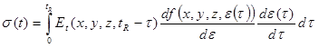
Figure 64. Equation. Nonlinear viscoelastic formulation for stress when relaxation modulus is separated from strain dependence function and when formulation is applied to a multilayered pavement structure.
Where Et(x,y,z,tR) is the relaxation function, and f(x,y,z, ε (τ))is a function of strain ε (τ) at location (x,y,z). Alternatively, to obtain vertical surface deflection in pavements, figure 64 can be expressed in terms of vertical deflection response to Heaviside step loading as shown in figure 65.

Figure 65. Equation. Nonlinear viscoelastic formulation for deflection.
Where:
uve(t) = the surface (nonlinear viscoelastic) displacement.
ueH-t (t, σ = 1) = the unit nonlinear elastic response due to a unit stress.
g(σ) = a function of stress, which can be expressed as shown in figure 66.
![]()
Figure 66. Equation. Nonlinear viscoelastic formulation.
Where ueH (tR , σ) is the nonlinear elastic unit displacement due to a given stress (σ). For Fung’s theory to hold (i.e., figure 63 through figure 66), g(σ) must be purely a function of stress. To investigate this, the g(σ) values were computed using figure 66 and plotted against surface stress and relaxation modulus (i.e., time). The LAVA algorithm was modified to implement an iterative nonlinear solution for the granular base, which was assumed to follow the following two nonlinearity expressions: MR = k1(θ /pa)k2 and MR = k1(θ /pa)k2(τ oct/pa + 1)k3. Analysis using the
k-θ-τ model is presented here whereas the k-θ model is presented in appendix A. The pavement section properties and material properties are shown in table 15 and figure 67.
Table 15. Pavement geometric and material properties for nonlinear viscoelastic pavement analysis.
| Property | Value |
|---|---|
| Thickness (inches) | 5.9 (AC), 9.84 (base), infinity (subgrade) |
| Poisson ratio (ν) | 0.35 (AC), 0.4 (base), 0.4 (subgrade) |
| Density (pci) | 0.0752 (AC), 0.0752 (base), 0.0752 (subgrade) |
| Nonlinear Ebase (psi) | k0 = 0.6; k1 = 3,626; k2= 0.5; k3 = -0.5 |
| Esubgrade (psi) | 10,000 |
| AC: E(t) sigmoid coefficient (ci) | 1.598, 2.937, 0.512, -0.562 |
| Haversine stress: 35 ms | Peak stress = 137.79 psi |
| Sensor spacing from the center of load (inches) | 0, 7.99, 12.01, 17.99, 24.02, 35.98, 47.99, 60 |

Figure 67. Diagram. Flexible pavement cross section for nonlinear viscoelastic pavement analysis.
The ueH (t, σ) in figure 66 was calculated at a range of stress values from 0.1 to 140 psi and using E(t) values for AC from 10-8 to 108 s. Then, ueH-t (t, σ = 1) was calculated for unit stress, and g(σ) was calculated using figure 66. Figure 68 shows the variation of g(σ), where the g(σ) values decrease with increasing stress (σ).

Figure 68. Graph. Variation of g(σ) with stress and E(t) of AC layer
This is expected behavior for a nonlinear material because as the stress increases, the unbound layer moduli also increase. However, figure 68 also illustrates that the g(σ) varies with change in E(t). This means that g(σ) is not solely based on the stress, and, as a result, Fung’s model cannot be used in a layered pavement structure. This is meaningful because the change in the stress distribution within the pavement layers due to viscoelastic effect (as E(t) varies) imposes changes in the behavior of stress-dependent granular layer. Note that as shown in appendix A, similar results were obtained when nonlinearity of k-θ type model was assumed. Hence, even though the viscoelastic layer in a nonlinear multilayered system is linear, it cannot be formulated as a Fung’s QLV model. The QLV model can still be formulated as a convolution integral, provided the stress-dependent relaxation function of the multilayered structure under all the load levels is known. Such a generalized QLV model for a multilayered structure can be expressed as nonlinear viscoelasticity equations involving the convolution integrals of unit response function of the structure, which is a function of stress or strain as shown in figure 69.

Figure 69. Equation. Generalized nonlinear viscoelastic formulation.
Where:
Rve(x,y,z,t) = the nonlinear viscoelastic response of the layered pavement structure.
ReH (x, y, z, I (τ), tR - τ) = the unit response function that is both a function of time.
input I(τ) = stress applied at the surface of the pavement.
Note that in this formulation, unlike Fung’s QLV model, time dependence and stress (or strain) dependence were not separated.
Figure 69 can be rewritten in terms of vertical surface deflection under axisymmetric surface loading (see figure 67) as shown in figure 70.

Figure 70. Equation. Generalized nonlinear viscoelastic formulation for deflection.
Where:
uvevertical (z,r,t) is the vertical deflection at time t and location (z,r).
ueH-vertical (z,r,σ(τ), tR - τ) = uevertical (z,r,σ(τ),tR - τ)/σ where
uevertical (z,r,σ,tR - τ) is the nonlinear response of the pavement at a loading stress level of σ.
The model in figure 70 can be expressed in discretized formulation as shown in figure 71.
![]()
Figure 71. Equation. Discretized nonlinear formulation.
Where τ1 = 0, τN = t. The ueH(σ, tRi - τj) values are computed via interpolation using the two-dimensional matrix pre-computed for ueH (t, σ) (which was computed at a range of stress values and E(t) values). The developed model has been referred to as LAVAN (short for LAVA-Nonlinear) in this report. The following step-by-step procedure can be used to numerically compute the response:
1. Define a discrete set of surface stress values: σk = 0.1 to 140 psi.
2. Calculate nonlinear elastic response ue(tRi, σk) at a range of tRi values, by using EAC = E(tRi) for each tRi value. Recursively compute Ebase until the stress in the middle of the base layer, at a radial distance r, results in the same Ebase as the one used in the layered elastic analysis (within acceptable error). For this step, the nonlinear formulation shown in figure 72 is assumed for the base.
![]()
Figure 72. Equation. Resilient modulus.
Where:
θ = σ1 + σ2 + σ3 + yz(1 + 2K0 ) (where K0 is the coefficient of earth pressure at rest).
τoct = octahedral shear stress.
k1, k2, and k3 = regression constants.
pa = atmospheric pressure.
3. ueH-vertical (r,z,ti,σk) =uevertical (r,z,ti,σk)σk
4. Perform convolution shown in figure 71 to calculate the nonlinear viscoelastic response.
To validate the LAVAN algorithm, ABAQUS was used. A flexible pavement was modeled as a three-layer structure, with a viscoelastic AC top layer over a stress-dependent granular base layer on an elastic half-space (subgrade). Figure 67 shows the geometric properties of the pavement structure used in the validation, where hAC = 5.9 inches and hbase=9.84 inches. The viscoelastic properties of two HMA mixes, called crumb rubber terminal blend (CRTB) and control (two materials from FHWA’s Accelerated Load Facility 2002 experiment) were used for the AC layer in the analysis as case 1 and 2, relaxation modulus master curve for the two mixes are shown in figure 73.(89) These curves were computed from their |E*| master curves by following the interconversion procedure suggested by.(58) The pavement properties in the analysis for each test case were the same, as shown in figure 15.

Figure 73. Graph. Relaxation moduli of mixes used in LAVAN validation.
In ABAQUS, the viscoelastic properties of the HMAs were input in the form of normalized bulk modulus (K) and normalized shear modulus (G).(90) For the unbound nonlinear layer, a UMAT was written, incorporating the nonlinear constitutive modeling as explained in the previous section. ABAQUS requires that any UMAT have at least two main components: (1) update of the stiffness Jacobian Matrix and (2) stress increment. Figure 74 and figure 75 show the mathematical expressions for these two operations implemented in the UMAT.
![]()
Figure 74. Equation. ABAQUS Jacobian formulation.
![]()
Figure 75. Equation. ABAQUS stress update formulation.
Where J is the Jacobian matrix; σijn+1 is the updated stress; and i, j, k, and l represent r, z, t, and θ in the cylindrical coordinate system. For nonlinear analysis using LAVAN, the unbound modulus was calculated using the stress state at the midpoint of the unbound base layer (vertically). Because LAVAN cannot incorporate nonlinearity along the horizontal direction, for comparison, modulus values were calculated using stress at r = 3.5a (r shown in figure 67). In ABAQUS, the FE domain size of 133R in the vertical direction and 53R in the horizontal direction was found to produce stable surface deflection (with less than 1-percent error at the center). For the selected domain size, the FEM mesh refinement of 0.4 inch in the AC layer and 1 inch in the base layer were used. ABAQUS took approximately 17 min to analyze a haversine loading of 138 psi and 35 ms, whereas LAVAN could generate the results in 3.6 min.
Comparison of surface deflection between LAVAN and ABAQUS for the control mix (figure 76) and CRTB mix (figure 77) shows good predictability of LAVAN. As expected, the stiffer mix (control) generated a lower response compared with the softer mix (CRTB) under the same geometric and loading conditions. The top graph in figure 76 shows the results when stress at r = 0 is used in LAVAN and was provided for comparison purposes. The bottom graph in figure 76 shows the results when stress at r = 3.5a was used in LAVAN. Note that S1, S2, S3, S4, S5, S6, S7, and S8 in the figures correspond to surface deflection Sensor-1 (r = 0 inches), Sensor-2 (r = 8 inches) etc. Sensors 1 through 8 were 0, 8, 12, 18, 24, 36, 48, and 60 inches away from the centerline of the load.

Figure 76. Graphs. Surface deflection comparison of ABAQUS and LAVAN for the control mix.

Figure 77. Graphs. Surface deflection comparison of ABAQUS and LAVA for the CRTB mix.
The difference between ABAQUS and LAVAN was quantified using the two variables shown in figure 78 and figure 79.

Figure 78. Equation. Error in peak deflection.

Figure 79. Equation. Average error in normalized deflection history.
Where:
PEpeak = Percent error in the peaks.
δ peakABACUS = Peak deflection predicted by ABAQUS.
δ peakLAVAN = Peak deflection predicted by LAVAN.
PEavg = Average percent error in normalized deflection history.
δABAQUS (ti) = Deflection predicted by ABAQUS at time ti.
δLAVAN (ti) = Deflection predicted by LAVAN at time ti.
N = Number of time intervals in the deflection time history.
Because the model integrates both viscoelastic and nonlinear material properties, both peak deflection and creeping of deflection should be predicted with accuracy. PEavg was used to examine the model performance in creeping.
As shown in figure 80 and figure 81, the PEpeak and PEavg values for the control mix showed a slight improvement in the results when r = 3.5a was used. However, from figure 82 and figure 83, it can be seen that PEpeak and PEavg values for CRTB mix showed more sensitivity to the location of the stress state.
In general, for the deflection basin at farther sensors, a better match between the ABAQUS and LAVAN results was found when stress state at r = 3.5a was used while incorporating nonlinearity. However, note that r = 0 also produced relatively good results, especially in the first four to five sensors. Also, note that, for the structure in table 15, the procedure leads to r = 2.8a when the trapezoidal stress distribution with (0.5 horizontal slope and 1 vertical slope) is assumed.(27)

Figure 80. Graph. Percent error (PEpeak) calculated using the peaks of the deflections for LAVAN-ABAQUS comparison (control mix).

Figure 81. Graph. Average percent error (PEavg) calculated using the entire time history for the LAVAN-ABAQUS comparison (control mix).

Figure 82. Graph. Percent error (PEpeak) calculated using the peaks of the deflections for the LAVAN-ABAQUS comparison (CRTB mix).

Figure 83. Graph. Average percent error (PEavg) calculated using the entire time history for the LAVAN-ABAQUS comparison (CRTB mix).
Backcalculation of pavement properties using FWD data is essentially an optimization problem. The analysis is based on formulating an objective function, which is minimized by varying the pavement properties. Response obtained from the forward analysis is matched with response obtained from the FWD test, and the difference is minimized by adjusting the layer properties of the system until a best match is achieved. Typically, the existing backcalculation methods either use RMS or percentage error of peak deflections as the objective function. However, because the viscoelastic properties are time dependent, the entire deflection history needs to be used. Hence, the primary component of the proposed backcalculation procedure was a layered viscoelastic forward solution. Such a solution should provide accurate and rapid displacement response histories owing to a time-varying (stationary) surface loading. For a linear viscoelastic pavement model, the research team used the computationally efficient layered viscoelastic algorithm LAVA to support the backcalculation algorithm called BACKLAVA, whereas for viscoelastic nonlinear pavement model, the team used the computationally efficient layered viscoelastic algorithm LAVAN to support the backcalculation algorithm called BACKLAVAN.(65)
Whenever mechanical properties are derived with inverse analysis, it is desirable to minimize the number of undetermined parameters by using an economical scheme. Such an approach is both advantageous from a computational speed perspective and addresses the non-uniqueness issue, i.e., test data may not be detailed, accurate, or precise enough to allow calibration of a complicated model. Moreover, it is beneficial to have some inherent “protection” within the formulation, forcing the analysis to a meaningful convergence—fully compliant with the physics of the problem. Therefore, as discussed before, the relaxation modulus (E(t)) master curve (figure 32) was initially assumed to follow a sigmoid shape defined by the equation in figure 84:
![]()
Figure 84. Equation. Sigmoid form of relaxation modulus curve.
Where ci are the sigmoid coefficients and tR is the reduced time, which is defined as tR = t/aT(T) (or log(tR) = log(t) – log(aT(T)), where, as discussed before (Figure 33), aT(T) is the shift factor coefficient, which is a function of temperature (T) and t is time. The shift factor coefficients has been defined as a second-order polynomial of the form log(aT(T)) = a1(T2–Tref2) + a2(T – Tref), where a1 and a2 are the shift factor coefficients. As shown by the relaxation modulus and shift factor equations, a total of six coefficients were needed to develop the E(t) master curve, including the temperature dependency (i.e., the shift factor coefficients).
In theory, it should be possible to obtain these six coefficients in two ways: (1) using data containing time-changing response at different temperature levels and (2) using uneven temperature profile information existing across the thickness of the asphaltic layer during a single drop containing time changing response data.
Reliability and accuracy of the backcalculated results depend on the optimization technique used. In the present work, several optimization techniques were tried to formulate a procedure to backcalculate these six viscoelastic properties along with unbound material properties. These optimization techniques can be broadly classified as classical methods and evolutionary methods. In this study, simplex-based classical optimization method was performed using MATLAB® function fminsearch, whereas, genetic algorithm (GA)-based evolutionary optimization method was performed using the MATLAB® function ga. The objective function, which is based on deflection differences in the current work, is a multidimensional surface that can include many local minima. In elastic backcalculation methods, the modulus of the AC layer is defined using a single value. However, in the present problem, the AC properties were represented by a sigmoid containing four parameters for E(t) and by a polynomial containing two parameters for aT(T). Hence, it was naturally expected that the probability of number of local minima would increase. In traditional methods, because of the presence of multiple local minima, selection of different initial solutions may lead to different subsequent solutions. Typically, classical optimization methods (such as the fminsearch) have the following issues:
These disadvantages do not mean that classical methods cannot be used in the backcalculation procedure. In fact, the classical methods can be hybridized along with evolutionary optimization techniques in developing more effective backcalculation procedures.
It is important to develop a backcalculation process such that FWD data obtained at a relatively small range of pavement temperatures can be sufficient to derive the viscoelastic properties of AC. Among various optimization techniques, GA was chosen because of its capability to converge to a unique global minimum solution, irrespective of the presence of local solutions.(91–93) GA was implemented using MATLAB® function ga. In general terms, GA performs the following operations: (1) initialization, (2) selection, (3) generation of offspring, and (4) termination. In initialization, GA generates a pool of solutions using a subset of the feasible search space, the so-called “population.” Each solution is a vector of feasible variable values. In the selection process, each solution is evaluated using an objective function, and the best fitted solutions are selected. The selected solutions are then used to generate the next generation population (offspring). This process mainly involves two operators: crossover and mutation. In crossover, a new solution is formed by exchanging information between two parent solutions, which is done by swapping a portion of parent vectors. In mutation, a new solution is formed by randomly changing a portion of the parent solution vector. The newly generated population is evaluated using the objective function. This process is repeated until a termination criterion is reached. Through guided random search from one generation to another, GA minimizes the desired objective function.
Formulation of the optimization model using GA is shown in figure 85.

Figure 85. Equation. Optimization model.
Where:
m = Number of sensors.
di = Input deflection information obtained from field at sensor k.
dok = Output deflection information obtained from forward analysis at sensor k.
n = Total number of deflection data points recorded by a sensor.
ci = Sigmoid coefficients.
Eb and Es = Base and subgrade moduli.
ai = Shift factor polynomial coefficients.
l = Lower limit.
u= Upper limit.
This model is also subject to the following constraints:
and
To obtain the lower and upper limits of ci and ai, values of sigmoid and shift factor coefficients of numerous HMA mixtures were calculated. Table 16 shows these limits, which were used in the GA constraints shown in figure 85. Limits to the elastic modulus were arbitrarily selected (based on typical values presented in the literature). Note that the sigmoid obtained by using the lower or upper limits of the coefficients gave a larger range compared with the actual range of E(t). This could potentially slow down the backcalculation process. Therefore, as described later in the report, additional constraints were defined to narrow the search window.
Table 16. Upper and lower limit values in backcalculation.
| Limit | c1 | c2 | c3 | c4 | a1 | a2 | E1 | E2 |
|---|---|---|---|---|---|---|---|---|
| Lower | 0.045 | 1.80 | -0.523 | -0.845 | -5.380E-04 | -1.598E-01 | 10,000 | 22,000 |
| Upper | 2.155 | 4.40 | 1.025 | -0.380 | 1.136E-03 | -0.770E-01 | 13,000 | 28,000 |
The duration of a single pulse of an FWD test is very short, which limits the portion of the E(t) curve used in the forward calculation using LAVA. As a result, it was not possible to backcalculate the entire E(t) curve accurately using deflection data of such short duration. The longer the duration of the pulse, the larger portion of the E(t) curve used in LAVA in the forward calculation process. Therefore, one may conclude that FWD tests need to produce a long-duration deflection-time history. However, owing to the thermorheologically simple behavior of AC, the time-temperature superposition principle can be used to obtain longer duration data by simply running the FWD tests at different temperatures and using the reduced time concept described at beginning of this chapter.
Before discussing into the details of the required number of FWD test temperatures and magnitudes, an analysis on the effects of different FWD deflection sensor data on the backcalculated E(t) master curve is presented in the following section.
This section presents an analysis of the contribution of individual and a group of sensors on the backcalculation of the E(t) master curve. Note that the analysis was based on a real coded GA, which uses double vector variables. All the existing applications of GA in pavement inverse analysis were based on a binary coded GA, and hence the GA parameters suggested in these references were not applicable to the approach presented in this section.(91–93) As a result, a new set of optimum parameters was determined. The backcalculation process was run using a population and generation of 70 and 15, respectively (selected after trying various combinations), using FWD time histories obtained at a temperature set of {32, 50, 68, 86, 104, 122, 140, 158, and 176} °F. The pavement properties used (see table 17) were kept the same throughout the study.
Table 17. Pavement properties in viscoelastic backcalculation of optimal number of sensors.
| Property | Case 1 |
|---|---|
| Thickness (AC followed by granular layers) (inches) | 10, 20, infinity |
| Poisson ratio {layer 1,2,3…} | 0.35, 0.3, 0.45 |
| Eunbound {layer 2,3…} (psi) | 11,450, 15,000 |
| E(t) sigmoid coefficient {layer 1} | 0.841, 3.54, 0.86, -0.515 |
| a(T) shift factor polynomial coefficients {layer 1} | 4.42E-04, -1.32E-01 |
| Sensor spacing from the center of load (inches) | 0, 8, 12,18,24, 36,48, 60 |
Convergence was evaluated based on the backcalculated moduli of the base and subgrade layers as well as the E(t) curve of the AC layer. Average error in the moduli of base and subgrade are defined as shown in figure 86.
![]()
Figure 86. Equation. Average error in backcalculated moduli of base and subgrade layers.
Where:
ξunbound = Absolute value of the error in the backcalculated unbound layer modulus.
Eact and Ebc are the actual and backcalculated moduli (of the unbound layer), respectively.
The variation of error in the backcalculated E(t) at different reduced times is defined as shown in figure 87.
![]()
Figure 87. Equation. Error in backcalculated relaxation moduli at different reduced times.
Where:
ξAC(ti) = E(t) error at reduced time ti, where i ranges from 1 to n such that t1 = 10-8 and tn = 108 s.
n = Total number of discrete points on the E(t) curve.
Eact(ti) = Actual E(t) value at point i.
Ebc(ti) = Backcalculated E(t) value at i.
Finally, average error in E(t) is defined as shown in figure 88.

Figure 88. Equation. Average error in backcalculated relaxation moduli.
Where ξavgAC is the average error in the E(t) of the AC layer.
Figure 89 shows the variation of ξunbound when data from different FWD sensors are used. As shown, the error decreased as data from farther sensors were incorporated in the backcalculation. This may be because at farther sensors, the deflections were primarily, if not solely, due to deformation in the lower layers.

Figure 89. Graph. Error in unbound layer modulus in optimal number of sensor analysis.
Figure 90 shows the actual and backcalculated E(t) curve, which is only based on data from sensor 1 (at the center of load plate). As shown, there was a very good match between the backcalculated and actual curves. Figure 91 shows the variation of percentage error in E(t) (calculated using figure 87) with time. The magnitude of percent error ranged from about -9 to 23 percent and increased with reduced time. This was expected because the E(t) in longer durations (> 10-6 s) were not used in the forward computations. Note that the result is shown over a time range of 10-8 to 108 s. However, the forward calculations were actually made using temperatures ranging from 32 to 176 °F, which corresponded to a reduced time range of approximately 10-6 to 106 s.
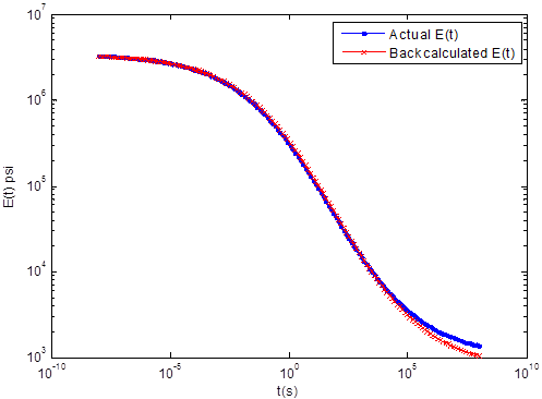
Figure 90. Graph. Backcalculated and actual E(t) master curve at the reference temperature of 66 °F using FWD data from only sensor 1.

Figure 91. Graph. Variation of error when using FWD data from only sensor 1.
To investigate whether using just the farther sensors improved the backcalculated Eunbound values, backcalculations were performed using data from different combinations of farther sensors. Figure 92 shows the error in backcalculation of the modulus of the base (layer 2) and the subgrade (Layer3), when data from only further sensors were used. As shown, for layer 3, error ranged between 0.27 to 1.43 percent, with no specific trend. The error in the modulus of the base (layer 2) was higher, ranging from 1 to 8.96 percent. However, a clear trend was not observed. By comparing with figure 89, one can conclude that using all the sensors produces the least error in Eunbound.

Figure 92. Graph. Error in unbound layer modulus using FWD data from only farther sensors.
It is typically not feasible to run the FWD test over a wide range of temperatures (e.g., from 32 to 176 °F). Depending on the region and the month of the year, the variation of temperature in a day can be anywhere between 50 and 86 °F during the fall, summer, and spring when most data collection is done. This means that the performance of the backcalculation algorithm needs to be checked for various narrow temperature ranges. The purpose of the study explained in this section was to determine the effect of different temperature ranges on the backcalculated E(t) values. Further, it was recognized that the results obtained from GA might not be exact but only an approximation of the overall solution. Hence a local search method was carried out through fminsearch using the results obtained from GA as seed. Figure 93 shows the error in the backcalculated elastic modulus values of base and subgrade when different pairs of temperatures were used. As shown, in most cases, the error was less than 0.1 percent. Note that the errors shown in figure 93 were less than the ones shown in figure 89 (when all sensors were used). This was because in figure 89, only GA was used, whereas in figure 93, fminsearch was used after the GA, which improved the results.

Figure 93. Graph. Variation of error in backcalculated unbound layer moduli when FWD data run at different sets of pavement temperatures are used.
Figure 94 shows the average error in E(t) (i.e., ξavgAC given in figure 88), where a pattern was observed. The error was the least when intermediate temperatures (i.e., {50-68}, {50-68-86}, {68-86-104}, {86-104}, {86-104-122} °F) were used. At low temperatures, the error seemed to increase. This was meaningful because at low temperatures, a small portion (upper left in figure 90) was used in BACKLAVA. Therefore, the chance of mismatch at the later portions of the curve (lower right in figure 90) was high. At high temperatures, error also seemed to increase. Theoretically, the higher the temperature, the larger the portion of the E(t) curve that was used because of the nature of the convolution integral, which starts from zero (figure 29). However, if only the high temperatures were used, the discrete nature of load and deflection time history led to a big jump from zero to the next time ti, during evaluation of the convolution integral. This jump occurred because when the physical time at high temperatures was converted to reduced time, actual magnitudes became large and, in a sense, a large portion at the upper left side of the E(t) curve was skipped during the convolution integral. At intermediate temperatures, however, a more balanced use of the E(t) curve in BACKLAVA improved the results.

Figure 94. Graph. Error in backcalculated E(t) curve in optimal backcalculation temperature set analysis minimizing percent error.
When results from GA were used as seed values in fminsearch, it was observed that in general, error in E(t) was reduced. Figure 95, figure 96, and figure 97 show backcalculated E(t) master curve using GA and corresponding backcalculated E(t) master curves obtained using GA and fminsearch. As shown, combined use of GA and fminsearch resulted in improved backcalculation.

Figure 95. Graphs. Results for backcalculation at {50, 86} °F temperature set: left side—only GA used, right side—GA+fminsearch used.

Figure 96. Graphs. Results for backcalculation at {86, 104} °F temperature set.

Figure 97. Graphs. Results for backcalculation at {86, 104, 122} °F temperature set.
Table 18 shows the time it takes to run the GA for population-generation size of 70 to 15, followed by fminsearch. The results are shown for a computer that has Intel Core 2, 2.40 GHz, and 1.98GB RAM.
Table 18. Backcalculation runtime for GA-fminsearch seed runs.
| Number of Temperature Data |
Backcalculation time (min) |
|---|---|
| Two (e.g., {50, 86}°F) | 30 |
| Three (e.g., {50, 68, 86} °F) | 40 |
| Seed run (fminsearch) | 15–20 |
In the analysis presented in the previous sections, percent error between the computed and measured displacement was used as the minimizing error. However, the deflection curve obtained from the field often includes noise, especially after the end of load pulse. If percent error is used as the minimizing objective, it may lead to overemphasis of lower magnitudes of deflections at the later portion of the time history, which typically includes noise and integration errors. Hence, another fit function was proposed in which the percent error was calculated with respect to the peak of deflection at each sensor. This approach penalized the tail data by normalizing it with respect to the peak, as shown in figure 98.

Figure 98. Equation. Normalized error in deflection history.
Where:
{d k}max = Peak response at sensor k.
m = Number of sensors.
dik = Measured deflection at sensor k.
dok = Output (calculated) deflection from forward analysis at sensor k.
n = Total number of deflection data points recorded by a sensor.
The limits considered for E(t) so far were the limits on the individual parameters of the sigmoid curve (table 16). The E(t) curves obtained by considering the upper and lower limits of the parameters represent curves well beyond the actual data base domain. To curtail this problem, constraints were introduced putting limits shown in figure 99 on the sum of the sigmoid coefficients c1 and c2.
![]()
Figure 99. Equation. Constraints in optimization model.
Where s1 and s2 are arbitrary constants.
The arbitrary constants s1 and s2were obtained by calculating maximum and minimum values of the sum of sigmoid coefficients c1 and c2 from numerous HMA mixes. Alternatively, the problem was reframed by incorporating the constraints in limit form by redefining the variables as shown in figure 100.

Figure 100. Equation. Sigmoid variables in optimization model.
Where c1 through c4 are sigmoidal function coifficents, and xu and x1 are the upper and lower limits of c1 + c2, respectively. The problem was then resolved after replacing the inequality constraint with limits on the variables. The new function gave good results at temperature sets of {50, 86} °F, {86, 104} °F, {50, 68, 86} °F, {68, 86, 104} °F, and {86, 104, 122} °F. The backcalculated E(t) curves were then converted to |E*| using the interconversion relationship given in Kutay et al.(65) Mathematically, the dynamic modulus can be defined as shown in figure 101:
![]()
Figure 101. Equation. Dynamic modulus in complex form.
Where f is frequency, E'(f) is storage modulus, and E"(f) loss modulus, which can be obtained for a generalized Maxwell model using the following equations shown in figure 102 and figure 103:

Figure 102. Equation. Real component of dynamic modulus.

Figure 103. Equation. Imaginary component of dynamic modulus.
Where:
Φ = the phase angle.
|E*| = the absolute value of the complex E* function (figure 101).
Ei = modulus of each Maxwell spring.
ρi = ηi /Ei = relaxation time
ηi = the viscosity of each dashpot element in the generalized Maxwell model as shown in figure 104.
![]()
Figure 104. Equation. Dynamic modulus and phase angle.
Backcalculated E(t) and |E*| master curves were compared with the actual curves for temperature sets {50, 86} °F and {50, 68, 86} °F in figure 105 and figure 106, respectively.

Figure 105. Graph. Backcalculated |E*| master curve using FWD data at temperature set {50,86} °F, minimizing normalized error.

Figure 106. Graph. Backcalculated E(t) master curve using FWD data at temperature set {50-68-86} °F, minimizing normalized error.
It can be seen from figure 107 that the results obtained for E(t) errors over temperature sets showed a distinct pattern. The E(t) and Eunbound errors with respect to temperature sets showed a trend similar to that observed in the case of percentage error (figure 93 and figure 94, respectively). The error was observed to be high at sets of low ({32, 50} °F) and high ({122,140} °F, {104, 122, 140} °F, {122, 140, 158} °F) temperatures. This is because the backcalculated E(t) at lower temperatures represents the left portion of the sigmoidal E(t) curve and higher temperatures represents the right. As explained earlier, both regions are fairly flat and hence represent constant values of E(t), which may not optimize to the actual E(t) curve. Better results were obtained for the temperature range of {50, 68} °F to {86, 104, 122} °F (figure 108). The backcalculated E(t) master curves and corresponding errors obtained at {50, 86} °F and {68,86, 104} °F for the proposed backcalculation model are shown in figure 109.

Figure 107. Graph. Variation of ξavgAC at different FWD temperature sets

Figure 108. Graph. Variation of ξ unbound at different FWD temperature sets

Figure 109. Graphs. Backcalculation results obtained using modified sigmoid variables.
In the previous sections, analyses were performed using only a single mix. To verify the conclusions made in the previous sections regarding the optimum range of temperatures of FWD testing, backcalculations were performed on nine typical mixtures. Actual viscoelastic properties—relaxation modulus and shift factors of the selected mixtures—are shown in figure 110.

Figure 110. Graphs. Viscoelastic properties of field mix in optimal temperature analysis.
Comparison of the average error in the backcalculated relaxation modulus function calculated over three time ranges—10-5 to 1 s, 10-5 to 102 s, and 10-5 to 103 s—as shown in figure 111. It can be seen from the figure that, for all the mixes, relaxation modulus curve can be predicted close to less than 15 percent over a range of relaxation time less than 10+3 s. Furthermore, it can be seen that, as suggested, the backcalculated relaxation modulus prediction provided a good match over an approximate temperature range of 50 to 86 °F.

Figure 111. Graphs. Variation of error calculated over three ranges of reduced time—top = 10-5 to 1 s, middle= 10-5 to 102 s, and bottom = 10-5 to 103 s.
In theory, it should be possible to obtain a relaxation modulus master curve if data containing the time-changing response at different temperature levels were known. The available analysis window in the current FWD devices is short, extending up to 25 to 35 ms of stress pulse, which could be used to infer part of the relaxation function. Although series of FWD tests at different temperatures could be useful in developing the entire master curve, in theory, the prediction could be improved if information at different rates of loading or over a larger time interval were known.
As shown in figure 112, a load of four successive pulses with a duration of 35 ms followed by four pulses with 10s duration each was simulated to generate the deflection basin. This example was used to investigate whether a different loading history could result in better estimation of E(t). Figure 113 shows the backcalculated E(t), where a good fit is visible. Note that the accuracy of the backcalculated E(t) depended on the duration of the stress pulse, where longer duration allowed calculation of E(t) at longer durations. It is also important to apply a high-frequency (short duration) pulse load to increase the accuracy of E(t) at very short times. Note that backcalculation of E(t) for this example took less than 5 min in the MATLAB® optimization tool fminsearch. These possibilities are explored in detail in appendix B.

Figure 112. Graphs. Applied stress and resulting deflection basin for multiple pulse loading analysis.

Figure 113. Graph. Backcalculated E(t) and deflection histories using the multiple stress pulses.
The uneven temperature profile existing across the thickness of the AC layer during a single FWD drop can theoretically be used to backcalculate the E(t) master curve and the shift factor coefficients (aT(T)). The AC layer can be divided into several sublayers with same viscoelastic properties but with different temperature levels. Two different approaches of backcalculation are discussed in this section. In the first approach, all the unknown variables (sigmoid coefficients, shift factor coefficients, and unbound modulus) in the forward algorithm were varied during backcalculation. In the second approach, a two-staged backcalculation procedure was adopted. The two-stage method involved static backcalculation in the first stage (unbound modulus assuming elastic AC layer) followed by viscoelastic backcalculation in the second (sigmoid and shift factor coefficients). Both approaches were explored in the present study.
As discussed earlier, a total of six coefficients are needed to represent the relaxation properties of the AC layer, including the temperature dependency. The backcalculation procedure used was same as used in the previous section (i.e., BACKLAVA), except the forward analysis was replaced by LAVAP, which can consider varying temperature along the depth of the AC layer. Subsequently, the new backcalculation algorithm was referred as BACKLAVAP. For executing the GA, the same lower and upper limits of ci and ai (sigmoid and shift factor coefficients) and other specifications were retained.
As a first step, the backcalculation algorithm was validated with a synthetic FWD deflection history, under two different temperature profiles. The data were generated using LAVAP and then used in BACKLAVAP for backcalculation of E(t). The AC layer was divided into three equal sublayers with three different temperatures. Pavement section, properties, and temperature used in the forward analysis are shown in table 19.
Table 19. Details of the pavement properties used in single FWD test backcalculation under a known temperature profile.
| Property | Asphalt Concrete Layer | Granular Base |
Subgrade | |||
|---|---|---|---|---|---|---|
| Sublayer 1 |
Sublayer 2 |
Sublayer 3 |
||||
| Thickness (inches) | 2 | 2 | 2 | 20 | Semi-infinite | |
| Temperature (°F) | Case 1 | 68 | 59 | 50 | N/A | N/A |
| Case 2 | 86 | 77 | 68 | N/A | N/A | |
| Poisson’s ratio | 0.35 | 0.4 | 0.45 | |||
| Relaxation modulus | E(t) coefficients (c1, c2, c3, c4) backcalculated |
Backcalculated | Backcalculated | |||
| Time-temperature shifting coefficients | (a1, a2) backcalculated | N/A | N/A | |||
| Sensor spacing from the center of load (inches): 0, 8, 12, 18, 24, 36,48, 60 | ||||||
| N/A = Not applicable. | ||||||
For the case of backcalculation using a temperature profile, the GA parameters—population size and generation numbers—were again selected after several trials of combinations. It was observed that at population size of 300, improvement in the best solution was marginal after 12 to 15 generations, and the population converged to the best solution at about 45 generations. Similarly, for a population size of 400, improvement in the best solution was marginal after 10 to 15 generations. Figure 114 shows the backcalculation results at the temperature sets given in table 19, where a good match was visible. Error in the backcalculated E(t) was quantified relative to the actual E(t) using ξAC(ti), given in figure 87. The ξAC(ti) calculation was performed over a reduced time interval from 10-8 to 10+8 s. Then, the average error (ξ avgAC) was computed using figure 88. The average error level for the first temperature profile was found to be 5.2 percent, and for the second, it was 4.4 percent.
To further investigate the effect of the magnitude of the pavement temperature profile on backcalculation of E(t) master curve, synthetic FWD deflection histories were generated. The synthetic data were then used in backcalculation. The structure was divided into three layers with different temperatures, and E(t) was backcalculated using these data. The pavement section properties used in the study were same as shown in Table 19.
Backcalculation was performed assuming the temperature of the top, middle, and bottom sublayers of the asphalt layer as {68, 59, 50} °F, {86, 77, 68} °F, {104, 95, 86} °F, and
{122, 113, 104} °F. It was again observed that the problem converged well with 300 GA populations at 45 GA generations. The results shown in figure 115 did exhibit a trend, suggesting that there was a good potential for backcalculation of E(t) using a single FWD response for the lower temperature ranges, assuming that the temperature profile of the pavement was known.

Figure 114. Graphs. Comparison of actual and backcalculated values in backcalculation using temperature profile.
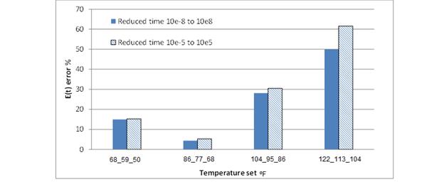
Figure 115. Graph. Error in backcalculated E(t) curve for a three-temperature profile.
The BACKLAVAP algorithm was next used with field data to backcalculate the viscoelastic properties of nine LTPP sections. With the exception of sections 10101, 300113, and 340801, selection of the sites was done based on the following rules:
Table 20 and table 21 contain general and structural information about each selected LTPP site. As shown in table 21, section 10101 had a total of four layers, including two AC layers. However, because the D(t) of the two AC layers reported in the LTPP database were very close, the section was included in the list, treating the two layers as a single AC layer in the analysis. Section 300113 comprised two AC layers of thickness 0.2 and 5.8 inches. Because the top AC layer of the section was very thin compared with the second AC layer, the AC layers were treated as a single layer. Furthermore, the sectional composition of sections 300113 and 340801 were not changed during various constructions; therefore, they were included in the analysis. However, it is not clear from the LTPP database whether the D(t) was measured before or after the constructions were done.
Table 20. List of LTPP sections used in the analysis.
| State | Section | Year of Construction |
Total Number of Constructions |
Section Type |
Experiment Number |
|---|---|---|---|---|---|
| 1 | 0101 | 4/30/1991 | 1 | SPS | 1 |
| 6 | A805 | 5/1/1999 | 1 | SPS | 8 |
| 6 | A806 | 5/1/1999 | 1 | SPS | 8 |
| 30 | 0113 | 9/18/1997 | 5 | SPS | 1 |
| 34 | 0801 | 1/1/1993 | 2 | SPS | 8 |
| 34 | 0802 | 1/1/1993 | 1 | SPS | 8 |
| 35 | 0801 | 9/11/1995 | 1 | SPS | 8 |
| 35 | 0802 | 9/11/1995 | 1 | SPS | 8 |
| 46 | 0804 | 1/1/1992 | 1 | SPS | 8 |
Table 21. Structural properties of the LTPP sections used in the analysis.
| State Code |
Section | Total Number of Layers |
Number of AC Layers |
AC Layer Thickness (inches) |
Base Layer Thickness (inches) |
|---|---|---|---|---|---|
| 1 | 0101 | 4 | 2 | AC1 = 1.2, AC2 = 6.2 |
7.9 |
| 6 | A805 | 3 | 1 | 3.9 | 8.2 |
| 6 | A806 | 3 | 1 | 6.8 | 12.1 |
| 30 | 0113 | 4 | 1 | AC1 = 0.2, AC2 = 5.8 |
8.4 |
| 34 | 0801 | 3 | 2 | 3.6 | 7.8 |
| 34 | 0802 | 3 | 1 | 6.7 | 11.6 |
| 35 | 0801 | 3 | 1 | 4.2 | 9.7 |
| 35 | 0802 | 3 | 1 | 7 | 12.7 |
| 46 | 0804 | 3 | 1 | 6.9 | 12 |
In the LTPP Program, each section is tested according to a specific FWD testing plan, which consists of one or more test passes. Both SPS 1 and SPS 8 are tested, along two test passes (test pass 1 and test pass 3) using test plan 4 in LTPP. Test pass 1 data include FWD testing performed along the midlane (ML) whereas test pass 2 data includes FWD testing performed along the OW path. Because testing with the ML test pass represents the axisymmetric assumption better, it was used here in the analysis. Furthermore, for each section, testing was done at several longitudinal locations (in the direction of traffic) in every test pass. Typically, for a 500-ft test section, FWD testing is performed at every 50 ft longitudinally along the test pass. In the LTPP testing protocol, temperature gradient measurements are taken every 30 min, plus or minus 10 min. The necessary temperature profile data were obtained by interpolating the temperature measured during the FWD testing. The AC layer was divided into three equal sublayers, and a constant temperature for each sublayer was estimated. Table 22 shows the interpolated temperatures at the middle of the three sublayers. From the table, it can be seen that the maximum temperature difference (between sublayer 1 and sublayer 3) was 11.2 °F in section350801 and the minimum 5.3 °F in section 6A805.
Table 22. AC temperature profile during LTPP FWD test.
| State Code |
Section | Test Date |
Temperature Profile (°F) | ||
|---|---|---|---|---|---|
| Sublayer 1 |
Sublayer 2 |
Sublayer 3 |
|||
| 1 | 0101 | 04/28/05 | 100.0 | 92.5 | 91.6 |
| 6 | A805 | 11/16/11 | 73.6 | 69.1 | 68.2 |
| 6 | A806 | 11/16/11 | 79.2 | 75.2 | 71.2 |
| 30 | 0113 | 07/12/10 | 84.7 | 80.1 | 79.2 |
| 34 | 0801 | 08/26/98 | 102.4 | 98.8 | 93.6 |
| 34 | 0802 | 08/26/98 | 79.3 | 83.3 | 86.5 |
| 35 | 0801 | 04/09/05 | 74.1 | 65.1 | 63.0 |
| 35 | 0802 | 05/26/00 | 89.8 | 84.4 | 83.3 |
| 46 | 0804 | 05/02/01 | 75.9 | 70.7 | 67.5 |
Except for section 350801, the FWD deflection data obtained showed no or minimal waviness at the end of the load pulse, which indicated that there was no shallow stiff layer. The FWD deflection data obtained from section 350801 showed some waviness at the end of the load pulse. This indicated the possibility of a medium-depth stiff layer or high water table. The presence of a stiff layer was further evaluated using a graphical method suggested by Ullidtz.(94) The method involves plotting peak deflections obtained from FWD testing versus the reciprocal of the corresponding sensor location (measured from the center of loading).(95) Depths of stiff layer in each LTPP section estimated using Ullidtz’s method are shown in table 23.(94) Note that negative depth to the stiff layer was interpreted as absence of the stiff layer in the method. The results indicate that stiff layers were generally deeper than 18 ft (except section 350801). It was suggested by Lei that if the stiff layer was below 18 ft, the effect of dynamics was not observed on the surface deflections.(96) Section 350801 was also included in the analyses because the depth of the stiff layer was close to the limit of 18 ft.
Table 23. Depths of stiff layer in each LTPP section estimated using Ullidtz’s method.
| State Code |
Section | Depth of Stiff Layer From Surface (ft) | |||
|---|---|---|---|---|---|
| Drop 1 | Drop 2 | Drop 3 | Drop 4 | ||
| 1 | 0101 | 86.9 | 32.7 | 109.8 | 26.6 |
| 6 | A805 | 70.4 | No stiff layer | No stiff layer | No stiff layer |
| 6 | A806 | No stiff layer | No stiff layer | No stiff layer | No stiff layer |
| 30 | 0113 | 96.4 | 45.3 | 49.9 | 35.6 |
| 34 | 0801 | 38.7 | 38.9 | 37.9 | 38.4 |
| 34 | 0802 | No stiff layer | No stiff layer | 284.5 | 63.8 |
| 35 | 0801 | 15.5 | 15.6 | 15.5 | 15.2 |
| 35 | 0802 | No stiff layer | No stiff layer | No stiff layer | No stiff layer |
| 46 | 0804 | 232.2 | 183.1 | 61.2 | 31.6 |
Section properties used for elastic and viscoelastic backcalculations were the same (see table 20) except that the modulus of the AC layer in the elastic backcalculation was assumed constant (modulus unknown). For elastic backcalculation, an in-house genetic algorithm was developed. The Poisson’s ratio for AC, granular base, and subgrade layers were assumed to be 0.3, 0.4, and 0.45, respectively. As noted above, the results obtained from elastic backcalculation were used to define bounds for base and subgrade moduli in BACKLAVAP. Table 24 shows the elastic backcalculation results obtained using data from each FWD drop. With the exception of section 350802, the static backcalculated base modulus values varied between 8,425 psi and 64,479 psi, and the subgrade modulus values varied between 16,142 psi and 42,615 psi.
Table 24. Elastic backcalculation results for LTPP sections.
| State Code |
Section | Drop 1 (psi) | Drop 2 (psi) | Drop 3 (psi) | Drop 4 (psi) | ||||
|---|---|---|---|---|---|---|---|---|---|
| Ebase | Esubgrade | Ebase | Esubgrade | Ebase | Esubgrade | Ebase | Esubgrade | ||
| 1 | 0101 | 34,129 | 46,835 | 29,941 | 45,478 | 36,065 | 42,122 | 22,264 | 42,615 |
| 6 | A805 | 44,302 | 19,612 | 44,985 | 19,533 | 44,176 | 19,707 | 64,479 | 19,599 |
| 6 | A806 | 32,252 | 23,219 | 29,063 | 23,281 | 34,932 | 22,511 | 43,687 | 22,636 |
| 30 | 0113 | 10,908 | 26,856 | 10,030 | 26,754 | 9,617 | 27,328 | 8,425 | 27,690 |
| 34 | 0801 | 19,853 | 20,918 | 19,446 | 21,150 | 26,287 | 21,392 | 26,063 | 22,062 |
| 34 | 0802 | 59,182 | 43,534 | 51,674 | 42,828 | 53,932 | 43,013 | 56,114 | 42,112 |
| 35 | 0801 | 25,508 | 23,061 | 20,762 | 22,567 | 20,995 | 21,738 | 22,113 | 21,649 |
| 35 | 0802 | 83,664 | 35,574 | 74,723 | 34,993 | 83,675 | 34,619 | 84,015 | 34,552 |
| 46 | 0804 | 19,699 | 16,142 | 23,137 | 16,207 | 18,359 | 16,282 | 13,676 | 16,545 |
Next, the viscoelastic backcalculation was performed. The backcalculated unbound layer moduli for the sections obtained from viscoelastic backcalculation are presented in table 25. For the viscoelastic backcalculation, the GA algorithm in BACKLAVAP used 300 populations in each of the 15 generations, except for sections 10101 and 350801, where a 400 population and 15 generations were used. However, Note that, for backcalculation, the search approximately converged after 10 generation for 300 populations. As shown in table 25, with the exception of section 350802, the static backcalculated base modulus values varied between 10,292 and 64,466 psi, and the subgrade modulus values varied between 17,114 and 44,906 psi. Comparing table 24 and table 25, it can be seen that the elastic and viscoelastic backcalculation predict similar modulus values for the unbound layers.
Table 25. Viscoelastic backcalculation results for LTPP sections.
| State Code |
Section | Drop 1 (psi) | Drop 2 (psi) | Drop 3 (psi) | Drop 4 (psi) | ||||
|---|---|---|---|---|---|---|---|---|---|
| Ebase | Esubgrade | Ebase | Esubgrade | Ebase | Esubgrade | Ebase | Esubgrade | ||
| 1 | 0101 | 28,799 | 44,906 | 26,431 | 44,035 | 28,026 | 42,682 | 25,621 | 41,470 |
| 6 | A805 | 44,377 | 17,523 | 44,929 | 17,114 | 44,928 | 18,234 | 43,871 | 18,436 |
| 6 | A806 | 26,977 | 21,273 | 24,441 | 20,724 | 28,809 | 20,903 | 29,150 | 22,615 |
| 30 | 0113 | 10,491 | 24,972 | 10,292 | 26,127 | 10,391 | 26,253 | 11,257 | 26,254 |
| 34 | 0801 | 22,337 | 20,569 | 20,282 | 19,901 | 18,243 | 20,569 | 14,824 | 22,710 |
| 34 | 0802 | 64,466 | 41,648 | 61,782 | 38,700 | 62,967 | 40,227 | 48,242 | 42,904 |
| 35 | 0801 | 22,337 | 20,569 | 20,282 | 19,901 | 18,243 | 20,569 | 14,824 | 22,710 |
| 35 | 0802 | 84,339 | 37,787 | 84,338 | 33,631 | 84,339 | 32,521 | 84,825 | 32,653 |
| 46 | 0804 | 26,191 | 14,746 | 17,922 | 14,827 | 15,427 | 15,125 | 12,575 | 16,373 |
Figure 116 shows example backcalculated (and measured) deflection time histories for sections 10101 and 350801, where section 10101 exhibited a better match than section 350801. This was attributed to the stiff layer being close to the 18-ft limit in section 350801.
To validate the backcalculated results, creep compliance data available in the LTPP database were converted into relaxation modulus E(t). Creep data were available in tabulated form at three temperatures—14, 41, and 77 °F—and seven different times—1, 2, 5, 10, 20, 50, and 100 s. Assuming the classical power law function for the creep compliance (figure 117), the available data were fitted separately to each temperature.

Figure 116. Graphs. Backcalculated and measured deflection time histories for LTPP sections10101 and 350801.
![]()
Figure 117. Equation. Creep compliance power law.
The associated relaxation modulus was then obtained using the mathematically exact formula given in figure 118.(85)
![]()
Figure 118. Equation. Relaxation modulus and creep compliance relationship.
Where D1 and n are the power function coefficients of D(t). The discrete relaxation modulus functions were then shifted to obtain a relaxation modulus master curve. Two different relaxation master curves were calculated. The first relaxation modulus master curve approximation was obtained when the time-temperature shift factors determined from the measured creep data were used to develop the relaxation master curve (labeled as “Measured 1”). The second relaxation modulus master curve approximation was obtained when the time-temperature shift factors determined from backcalculation were used to develop the relaxation master curve (labeled as “Measured 2”). This was done because laboratory creep compliance tests are usually not reliable in determining time-temperature superposition properties because a perfect stress-step function is very difficult to achieve in the laboratory and also because the results are contaminated with viscoplasticity, especially at the high temperatures and long creep times. Finally, for comparison, dynamic modulus and phase angle master curves were calculated from the relaxation modulus via interconversion.(65) For further verification, the estimated dynamic modulus obtained from ANN-based model ANNACAP was also compared. In the present work, all the estimated dynamic modulus master curve and time-temperature shift factors obtained from ANNACAP were based on the MR model in ANNACAP.(97) From the results, it was found that the dynamic modulus curves estimated using the ANNACAP model, especially at higher frequencies, agreed well with the dynamic modulus curves obtained through interconverted creep data. Backcalculated E(t) and aT(T) for the sections are shown in figure 119 to figure 127, and backcalculated dynamic modulus and phase angle are shown in figure 128 to figure 136. It can be seen from the figures that in general, the independent test drops within each section resulted in very similar predicted curves. Note that each FWD drop had a different load level and load history. Although the results were encouraging, backcalculated curves for sections 06A806, 350801, and 350802 showed noticeable disagreement with values derived from creep. However, although the dynamic modulus master curve predicted by ANNACAP matched well at the higher frequencies, it typically predicted higher values at reduced frequencies of less than 10-2 Hz.

Figure 119. Graphs. Comparison of measured and backcalculated E(t) and aT(T) for LTPP section 10101.

Figure 120. Graphs. Comparison of measured and backcalculated E(t) and aT(T) for LTPP section 6A805.

121. Graphs. Comparison of measured and backcalculated E(t) and aT(T) for LTPP section 06A806.

Figure 122. Graphs. Comparison of measured and backcalculated E(t) and aT(T) for LTPP section 300113.

Figure 123. Graphs. Comparison of measured and backcalculated E(t) and aT(T) for LTPP section 340801.

Figure 124. Graphs. Comparison of measured and backcalculated E(t) and aT(T) for LTPP section 340802.

Figure 125. Graphs. Comparison of measured and backcalculated E(t) and aT(T) for LTPP section 350801.

Figure 126. Graphs. Comparison of measured and backcalculated E(t) and aT(T) for LTPP section 350802.
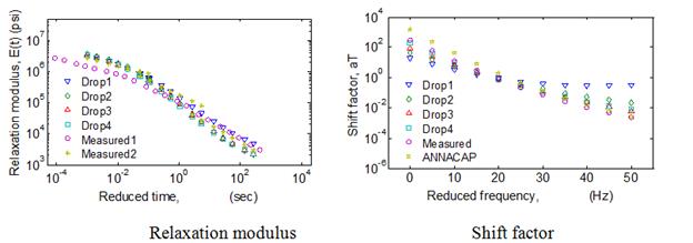
Figure 127. Graphs. Comparison of measured and backcalculated E(t) and aT(T) for LTPP section 460804.

Figure 128. Graphs. Comparison of measured and backcalculated |E*| and phase angle for LTPP section 10101.

Figure 129. Graphs. Comparison of measured and backcalculated |E*| and phase angle for LTPP section 6A805.
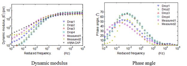
Figure 130. Graphs. Comparison of measured and backcalculated |E*| and phase angle for LTPP section 6A806.

Figure 131. Graphs. Comparison of measured and backcalculated |E*| and phase angle for LTPP section 300113.
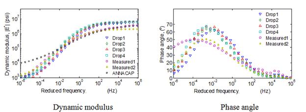
Figure 132. Graphs. Comparison of measured and backcalculated |E*| and phase angle for LTPP section 340801.

Figure Figure 133. Graphs. Comparison of measured and backcalculated |E*| and phase angle for LTPP section 340802.

Figure 134. Graphs. Comparison of measured and backcalculated |E*| and phase angle for LTPP section 350801.

Figure 135. Graphs. Comparison of measured and backcalculated |E*| and phase angle for LTPP section 350802.

Figure 136. Graphs. Comparison of measured and backcalculated |E*| and phase angle for LTPP section 46804.
As shown in figure 119, for section 10101, the relaxation modulus master curves matched very well when the time-temperature shift factor obtained from backcalculation was used (to shift the discrete relaxation modulus functions obtained through LTPP creep data) to develop a measured master curve (labeled as “Measured 2” in figure 119 (left)). On the other hand, when the time-temperature shift factors were determined from the measured creep data to develop the relaxation master curve (labeled as “Measured 2” in figure 119 (left)), there was a change from the backcalculated curves. The backcalculated time-temperature shift factors were compared with creep and ANNACAP-computed results in figure 119 (right). It can be seen from the figure that the backcalculated time-temperature shift factor functions for all the drops showed a good match over the temperature range of 50 to 131 °F. As shown in figure 128 (left), the backcalculated and measured dynamic modulus curve obtained from Measured 2 also matched well over the entire frequency range. The backcalculated phase angles were compared with measured results in figure 128 (right). The phase angles showed some deviation at frequencies less than 10-2 Hz. This was further verified by the dynamic modulus master curve estimated using ANNACAP, which showed a good match over a reduced frequency greater than 10-2 Hz.
For section 6A805, the backcalculated relaxation modulus master curves were compared with those measured in figure 120 (left). As shown in the figure, a better match with the backcalculated curves was found when the time-temperature shift factor obtained from the measured creep data was used to develop the measured master curve (labeled as “Measured 1” in figure 120 (left)). On the other hand, when the time-temperature shift determined from the backcalculation data was used to develop the relaxation master curve (labeled as “Measured 2” in figure 120 (left)), there was a change from the backcalculated curves. This disagreement in the time-temperature shift can also be seen in the time-temperature shift factors in figure 120 (right) and dynamic modulus and phase angle curves in figure 129.
Relaxation modulus and time-temperature shift factor curves for section 6A806 were compared in figure 121 (left) and figure 121 (right), respectively. For this section, the measured relaxation modulus master curves predicted higher values compared with the backcalculated results, which increased with reduced time. Both the predicted aT(T) curved obtained from ANNACAP and backcalculation deviated from the measured results. From figure 130 (left) and figure 130 (right), it can be seen that the deviation in relaxation modulus values with time was reflected in dynamic modulus and phase angle curves at lower frequencies.
Relaxation modulus and time-temperature shift factor curves for section 06A806 were compared in figure 122 (left) and figure 122 (right), respectively. Although the predicted aT(T) curve at drop 1 for section 300113 showed some deviation after 86 °F, both the backcalculated E(t) and aT(T) curves showed good agreement with laboratory results as well as ANNACAP data. Although the dynamic modulus predicted for drop 1 (see figure 131) showed lower values at frequencies greater than 102 Hz, an agreement in backcalculated relaxation modulus curves was also reflected in the dynamic modulus and phase angle curves.
Relaxation modulus and time-temperature shift factor curves for sections 340801 and 340802 were compared in figure 123 and figure 124, respectively. Although the predicted E(t) curves for sections 340801 and 340802 showed some deviation at reduced time greater than 10 s, in general, the two curves showed good agreement with the measurement. Comparison of the backcalculated aT(T) curves for both sections 340801 and 340802 (see figure 123 (right) and figure 124 (right)) show a good agreement with ANNACAP and measured curves over the temperature range of 50 to 104 °F. Further, it can be seen from figure 132 and figure 133 that although the dynamic modulus and phase angle curves predicted by individual drops were the same, deviation at reduced time greater 101 s in relaxation modulus was reflected at frequencies greater than 10-1 Hz.
Figure 125 shows the backcalculated E(t) and aT(T) functions for section 350801. Similar results were obtained using drops 1, 3, and 4, whereas E(t) from drop 2 deviated from the other drops. The reason for this deviation may be the relatively low base modulus (20,241 psi) backcalculated using this drop, as seen in table 25. The average of base moduli in drops 1, 3, and 4 was 28,468 psi, which is about 40-percent higher than the above base modulus value of drop 2. As shown in figure 126 (left) and figure 126 (right), comparison of backcalculated E(t) and aT(T) curves with measured and ANNACAP results for section 350802 showed complete disagreement. As shown in figure 135 (left) and figure 135 (right), similar discrepancies were reflected in the dynamic and phase angle curves.
For section 46804, the backcalculated relaxation modulus master curves were compared with measured results in figure 127 (left). It can be seen from the figure that the relaxation modulus master curves matched very well when the time-temperature shift factor obtained from backcalculation was used to develop the measured master curve (labeled as “Measured 2” in figure 127 (left)). On the other hand, when the time-temperature shift determined from the measured creep data was used to develop the relaxation master curve (labeled as “Measured 1” in figure 127 (left)), the backcalculated modulus values at reduced time less than 10-1 s were found to be low. Further, although the predicted aT(T) curve for drop 1 showed some deviation after 86 °F, the curves showed good agreement with laboratory as well as ANNACAP data. A comparison of backcalculated and measured dynamic modulus and phase angle for section 460804 is shown in figure 136 (left) and figure 136 (right), respectively. Dynamic modulus values predicted using backcalculation were higher at frequencies greater than 1 Hz, and a better prediction was observed with a frequency greater than 1 Hz.
Note that although measured creep data were used for comparison in the present study, it is not clear from the LTPP database whether D(t) was measured before or after the FWD tests were conducted.
In the previous backcalculation process, viscoelastic and unbound properties were calculated during the same step; however, in this section, a two-stage linear viscoelastic backcalculation scheme is presented. The first stage was to perform linear elastic backcalculation of unbound material properties, which was followed by linear viscoelastic backcalculation (using BACKLAVA/BACKLAVAP) of AC layer viscoelastic properties (E(t) sigmoid coefficients c1, c2, c3, and c4 and shift factor aT(T) coefficients a1 and a2). Details of stage 1 and stage 2 steps are presented in the following sections.
Stage 1: Elastic Backcalculation for Unbound Layer Properties
It is important to verify that the elastic backcalculation (stage 1) gives unbound granular modulus values close to the actual values. If this is verified, the backcalculated Eunbound values can be fixed in viscoelastic backcalculation (stage 2) and only the six unknowns of the AC layer can be backcalculated. Known and unknown variables in the first and second stages of backcalculation are listed in table 26. In stage1, elastic backcalculation was performed assuming the AC layer was linear elastic. In the stage 2, viscoelastic backcalculation was performed keeping the unbound granular layer modulus values obtained in the first stage fixed.
To perform the verification, first, various synthetic deflection time histories were obtained by running LAVA on the structure shown in table 27 at various temperature profiles (also shown in table 27). These synthetic deflections were used in stage 1, which computed Eunbound values. Then these backcalculated Eunbound values were compared with the original Eunbound values used in the original layered viscoelastic forward computation.
Table 26. Variables in two-stage linear viscoelastic backcalculation analysis.
| Stage | Known Parameters | Unknown (Backcalculated) Parameters |
|---|---|---|
| 1 | Thickness and Poisson’s ratio of each layer | Eac, elastic modulus of AC layer |
| FWD parameters (contact radius, pressure, locations of the sensors, etc.) |
Eunbound (i), unbound layer moduli, i = 1…NL, NL = number of unbound layers | |
| 2 | Thickness and Poisson’s ratio of each layer and FWD parameters |
E(t) sigmoid coefficients: c1, c2, c3, and c4 |
| Eunbound (i), unbound layer moduli backcalculated in stage 1 |
Shift factor aT(T) coefficients a1 and a2 |
Table 27. Pavement properties in two-stage linear viscoelastic backcalculation analysis.
| Property | Values |
|---|---|
| Thickness (AC followed by granular layers) (inches) | 6, 20, infinite |
| Poisson ratio {layer 1, 2, 3…} | 0.35, 0.3, 0.45 |
| Eunbound {layer 2, 3…} (psi) | 25,560, 11,450 |
| E(t) sigmoid coefficient {layer 1} | 0.841, 3.54, 0.86, -0.515 |
| aT(T) shift factor polynomial coefficients {layer 1} | 4.42E-04, -1.32E-01 |
| Total number of sensors | 8 |
| Sensor spacing from the center of load (inches) | 0, 8, 12, 18, 24, 36, 48, 60 |
| AC layer temperature profile {T1-T2} or {T1-T2-T3} (°F) |
{50-32}, {59-50}, {68-50}, {68-59}, {77-68}, {86-68}, {86-77}, {95-86}, {59-50-141}, {68-59-50}, {77-68-59}, {86-77-68}, {95-86-77}, {104-95-86} |
Figure 137 and figure 138 show the average base and subgrade modulus values obtained by elastic backcalculation of two- and three-step temperature profile, respectively. Error bars in the figures represent the standard deviation of 10 GA runs performed for each temperature set.

subg = subgrade.
Figure 137. Graph. Elastic backcalculation of two-step temperature profile FWD data, assuming AC as a single layer in two-stage backcalculation.

subg = subgrade.
Figure 138. Graph. Elastic backcalculation of three-step temperature profile FWD data, assuming AC as a single layer in two-stage backcalculation.
The analysis results shown in figure 137 and figure 138 were based on elastic backcalculations that assume a single AC layer. However, in the LAVA forward computations, because of different temperatures with depth, multiple layers of AC (two layers for Figure 137 and three layers for Figure 138 analysis) were used. To investigate whether selection of the number of AC layers affected the results for the elastic backcalculation, the computations were repeated assuming the AC layer consisted of two or three independent elastic layers. Average backcalculated base and subgrade modulus values for two-step and three-step temperature profiles are shown in figure 139 and figure 140, respectively. Comparing figure 137 with figure 139 and figure 138 with figure 140, it can be seen that assuming single or multiple AC layers did not significantly affect backcalculation of base and subgrade elastic modulus. From these analyses (figure 137 through figure 140), it can be concluded that it is possible to first perform elastic backcalculation (stage 1) for the unbound layer properties and fix these in stage 2.
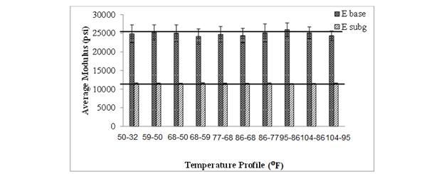
subg = subgrade.
Figure 139. Graph. Elastic backcalculation of two-step temperature profile FWD data, assuming two AC sublayers in two-stage backcalculation.

subg = subgrade.
Figure 140. Graph. Elastic backcalculation of three-step temperature profile FWD data, assuming three AC sublayers in two-stage backcalculation.
Stage 2: Viscoelastic Backcalculation for E(t) of AC Layer
After fixing the unbound layer modulus values, the AC layer properties (E(t) sigmoid coefficients: c1, c2, c3, and c4 and shift factor aT(T) coefficients a1 and a2) were backcalculated using the viscoelastic backcalculation algorithm (BACKLAVA). Note that for viscoelastic backcalculation, as done earlier, a set of FWD test data at different temperature can be used for backcalculation. This is because even though the temperatures are different, the characteristic properties of the AC layer (E(t) or |E*| master curves) remain the same. In this stage, viscoelastic backcalculation was performed on a set of temperature profiles keeping the actual unbound modulus values constant.
Average errors (over reduced times from 10-8 to 108 s) in the E(t) master curve, obtained from a set of two two-step and two three-step temperature profiles, are shown in figure 141 and figure 142, respectively. It can be observed from figure 141 that, for all the cases of the presented two-step temperature profile sets, average error in backcalculated E(t) was below 10 to 12 percent except for the FWD test at {86-68} and {104-86} °F. It can be observed from figure 142 that, for all the cases presented for the three-step temperature profile sets, average error in backcalculated E(t) was below 5.5 percent except for the FWD test at {86-77-68} and {77-68-59} °F. Subfigures in each of the figures were included to illustrate how the given percent error relates to the actual E(t) curves that were being compared. These results indicate that the two-stage algorithm worked well in backcalculating the E(t) of the AC layer. From figure 141 and figure 142, it can be observed that E(t) errors obtained in the two-stage backcalculation are less when compared with single-stage backcalculation (figure 120). However, note that results presented in figure 141 and figure 142 are from backcalculation using a set of two FWD test data each obtained at different temperature profiles, whereas results in figure 120 are from backcalculation using single FWD datum. However, the result does indicate that backcalculation using a set of FWD test data each obtained under a different temperature profile may improve the accuracy.

Figure 141. Graphs. Error in backcalculated E(t) curve from two-step temperature profile FWD test data in two-stage backcalculation.

Figure 142. Graphs. Error in backcalculated E(t) curve from three-step temperature profile FWD test data in two-stage backcalculation.
In the previous sections, the backcalculation scheme and results were developed for a viscoelastic multilayer pavement model consisting of a linear viscoelastic AC layer and linear elastic unbound layers. This section describes a backcalculation scheme (called BACKLAVAN) that was developed for the layered viscoelastic-nonlinear pavement model consisting of a linear viscoelastic AC layer and nonlinear elastic unbound layers. Because of computational limitations of the current version of the LAVAN algorithm, it can take a very long time to compute all the parameters (i.e., c1, c2, c3, and c4 of the AC and k1, k2, and k3 of the unbound layer) during the backcalculation stage. Therefore, a two-stage backcalculation scheme was proposed to backcalculate viscoelastic as well as nonlinear unbound layer properties of the pavement layers. The two-stage nonlinear backcalculation model was very similar to the two-stage linear backcalculation model discussed in the earlier section. In the nonlinear model, the first stage involved nonlinear elastic backcalculation of the properties (i.e., k1, k2, and k3) of the unbound granular layer. In the second stage, the backcalculated unbound properties (i.e., k1, k2, and k3) were fixed, and the layered viscoelastic-nonlinear model (LAVAN) was used to backcalculate the linear viscoelastic properties of AC layer. Details of known and unknown properties used during these two stages are shown in table 28. Note that the current forward algorithm (LAVAN) can easily be extended to include the nonlinearity of subgrade layers. However, when such forward solution was used in a backcalculation algorithm, computational efficiency decreased significantly. Typically, the effect of surface stress in the subgrade was limited (stress “bulb” effect) and assumption of linear elastic subgrade, with increasing E (due to geostatic stress) with depth may be sufficient for most design purposes.
Table 28. Pavement properties and test inputs in two-stage nonlinear viscoelastic backcalculation.
| Property | Stage 1: Nonlinear Elastic |
Stage 2: Nonlinear Viscoelastic |
|---|---|---|
| Thickness (inches) | Known (AC), known (BASE), infinite (SUBGRADE) | Known (AC), Known (BASE), infinite (SUBGRADE) |
| Poisson ratio | Known (AC), known (BASE), known (SUBGRADE) | Known (AC), Known (BASE), Known (SUBGRADE) |
| Ebase (psi) | Unknowns (k1, k2, k3) | Obtained from stage 1 |
| Egsubgrade(psi) | Unknown | Obtained from stage 1 |
| E(t)AC (psi) | Unknown (E(t) = constant) | Unknown (sigmoid coefficient) |
| Test Inputs | ||
| Surface loading (psi) | Known peak stress | Known load history |
| Surface deflection (inches) | Known peak deflection | Known deflection history |
The algorithm was used to backcalculate two HMA mixes, namely, Control and CRTB (for mix properties, refer to table 29), on a 35-ms haversine load (synthetic FWD pulse load). The section properties were as shown in table 29. Stresses at distance r = 0 (center of loading) and layer mid-depth were used in calculating unbound base modulus value for both forward calculation and backcalculation of synthetic data.
Table 29. Pavement geometric and material properties in two-stage nonlinear viscoelastic backcalculation.
| Property | Value |
|---|---|
| Thickness (inches) | 5.9 (AC), 9.84 (base), infinite (subgrade) |
| Poisson ratio (ν) | 0.35 (AC), 0.4 (base), 0.4 (subgrade) |
| Density (pci) | 0.0752 (AC), 0.0752 (base), 0.0752 (subgrade) |
| Nonlinear Ebase(psi) | Ko = 0.6; k1 = 3,626; k2 = 0.5; k3 = -0.5 |
| Esubgrade (psi) | 10,000 |
| AC: E(t) sigmoid coefficient (psi) (ci) |
Control: 1.598, 2.937, -0.272, -0.562 CRTB: 0.895, 3.411, 0.634, -0.428 |
| Shift factor coefficients (ai) | Control: 5.74E-04, -1.55E-01 CRTB: 4.42E-04, -1.32E-01 |
| Haversine stress 35 ms (psi) |
Peak stress = 137.79 psi |
| Sensor spacing from the center of load (inches): 0, 8, 12, 18, 24, 36, 48, 60 | |
Nonlinear elastic model is based on the assumption that the structure is time independent, with the AC layer assumed to be elastic and the unbound base layer assumed to be a stress-dependent nonlinear material. Each FWD test was generally composed of four independent test drops, where each drop corresponded to a different stress level. Typical ranges of stress levels in each drop are shown in table 30.
Table 30. Typical FWD test load levels.
| Load Level | Allowable Range for 11.81-inch Diameter Plate (psi) |
Used Surface Load (psi) |
|---|---|---|
| Drop 1 | 49–60 | 55 |
| Drop 2 | 74–96 | 80 |
| Drop 3 | 99–120 | 110 |
| Drop 4 | 132–161 | 137.8 |
In stage 1, peak stress and deflection values during all the test drops (drop 1 through 4) were used as input. Peak stress values in each drop (drops 1 through 4) for synthetic haversine FWD loading used in the present analysis were 55, 80, 110, and 138 psi, respectively (refer to table 30). The AC layer modulus and unbound layer properties (k1, k2, and k3) backcalculated from synthetic deflection at different temperatures are shown in figure 143 and figure 144, respectively.

Figure 143. Graph. Nonlinear elastic backcalculated AC modulus for control and CRTB mixes using FWD data at different test temperatures.
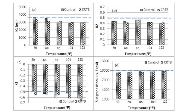
Figure 144. Graphs. Nonlinear elastic backcalculated unbound layer properties for control and CRTB mixes, using FWD data at different test temperatures.
As expected, for both control and CRTB mixes, the backcalculated elastic AC modulus values dropped with increase in temperature. Note that the forward solutions for the FWD surface deflections were computed using the LAVAN (layered viscoelastic-nonlinear) algorithm. The horizontal dashed lines in figure 144 show the actual inputs used in the LAVAN forward computation. As shown, the coefficients were close to the actual values but they were generally underpredicted by the backcalculation algorithm.
In stage 2, the backcalculated unbound layer properties from stage 1 were used as known fixed values, and the viscoelastic layer properties of the AC layer were obtained using viscoelastic-nonlinear backcalculation. The performance of the backcalculation algorithm was checked for the set of FWD data at temperatures ({50, 68}, {68, 86}, {86, 104}, {104, 122} °F) to determine the effect of different temperature ranges on the backcalculated E(t) values. The backcalculated unbound layer properties obtained in stage 1 at each independent temperature were averaged when a set of temperatures was used in viscoelastic backcalculation. Average error in the backcalculated E(t) master curve (refer to figure 145 and figure 146), (backcalculated in the second step) were calculated using figure 87. The error was calculated over four time ranges: (1)10-5 to 10+1 s, (2) 10-5 to 10+2 s, (3) 10-5 to 10+3 s, (4) and 10-5 to 10+5 s. From figure 145 and figure 146, it can be seen that for lower temperatures, the backcalculated E(t) master curve showed some deviation at higher reduced time, whereas, for higher temperatures, the backcalculated E(t) master curve showed some deviation at lower reduced time. The backcalculated results for the mixes showed good predictability of the E(t) master curve using the two-stage nonlinear backcalculation scheme.

Figure 145. Graphs. Control mix backcalculation results from two-stage nonlinear viscoelastic backcalculation.

Figure 146. Graphs. CRTB mix backcalculation results from two-stage nonlinear viscoelastic backcalculation.
The developed two-stage backcalculation algorithm was next used with field data to backcalculate the viscoelastic properties of the LTPP section 0101 from State 1 (Alabama). Section10101 was tested consecutively in 2004–2005, with the two tests separated by more than 68 °F (refer to table 31 and table 32). Further, because the section was not modified between the two tests, it was selected for the analysis.
Table 31. FWD test data from LTPP section 10101 for 2004–2005.
| Test Date | Drop Level | Peak Stress (psi) | Deflection (mil) | ||||||
|---|---|---|---|---|---|---|---|---|---|
| 2/23/2004 | 1 | 54.1 | 5.00 | 4.25 | 3.70 | 2.99 | 2.44 | 1.57 | 1.10 |
| 2 | 83.5 | 8.11 | 6.93 | 6.10 | 4.92 | 4.06 | 2.56 | 1.81 | |
| 3 | 113.3 | 11.65 | 10.00 | 8.82 | 7.13 | 5.87 | 3.78 | 2.60 | |
| 4 | 148.7 | 16.14 | 13.90 | 12.17 | 9.92 | 8.19 | 5.24 | 3.62 | |
| 4/28/2005 | 1 | 52.2 | 8.90 | 6.46 | 5.04 | 3.54 | 2.48 | 1.46 | 0.94 |
| 2 | 80.2 | 13.98 | 10.47 | 8.50 | 5.83 | 4.17 | 2.40 | 1.73 | |
| 3 | 111.2 | 20.20 | 15.55 | 12.91 | 8.90 | 6.38 | 3.74 | 2.76 | |
| 4 | 139.1 | 26.06 | 20.28 | 16.93 | 11.81 | 8.39 | 4.84 | 3.50 | |
In stage 1, peak stress and deflection values during all the test drops in table 31 were used as inputs in nonlinear elastic backcalculation. The backcalculation results in table 32 show that the unbound base properties (k1, k2, and k3) were found to be very close; it also shows that although the AC was affected by the temperature of the test, the effect on the unbound layer was not significant. As expected, the backcalculated elastic AC modulus values dropped with increase in temperature.
Table 32. Nonlinear elastic backcalculation results for LTPP section 10101.
| Results | FWD Test Year | ||
|---|---|---|---|
| 2004 | 2005 | ||
| Average AC temperature (°F) | 53.4 | 95.4 | |
| Properties | AC modulus (psi) | 941,526 | 227,346 |
| k1 | 17,984 | 15,972 | |
| k2 | 0.16 | 0.17 | |
| k3 | -0.59 | -0.58 | |
| Esubg | 29,832 | 26,097 | |
Unbound layer material properties may vary depending on environmental factors (seasons). However, because the unbound layer properties obtained for the two tests in stage 1 were found to be very close, they were used in the second stage of the backcalculation without any correction. Stage 2 uses the nonlinear viscoelastic forward algorithm during backcalculation of the E(t) of the AC layer. Note that viscoelastic backcalculation requires the entire time history for backcalculation. For the LTPP section test in year 2004, the entire deflection history was available only for drop 1, hence the backcalculation was performed using only drop 1. Figure 147 and figure 148 show results obtained by two independent backcalculation attempts using data from 2 years of field testing. As shown, a very good match was seen in E(t), and a reasonable match was seen in the shift factor function. The measured viscoelastic properties in the figures were obtained using D(t) data available in the LTPP database (refer to figure 117 and figure 118). As explained earlier (refer to figure 101 through figure 104), the dynamic modulus and phase angle master curve for the backcalculated E(t) were calculated at 66 °F.

Figure 147. Graphs. Comparison of nonlinear viscoelastic backcalculated and measured E(t) and aT(T) for LTPP section 10101.

Figure 148. Graphs. Comparison of nonlinear viscoelastic backcalculated and measured |E*| and phase angle for LTPP section 10101.
This chapter presented two methodologies for determining the E(t)/|E*| master curve and unbound material properties of in-service pavements. As part of this effort, two multilayered viscoelastic algorithms were developed. The first algorithm, called LAVA/LAVAP (LAVA can consider constant AC layer temperature, and LAVAP can consider a temperature profile for the AC layer), assumed the AC layer was a linear viscoelastic material and the unbound layers was linear elastic. The second algorithm (called LAVAN) also assumed the AC layer was a linear viscoelastic material; however, it can consider the nonlinear (stress-dependent) elastic moduli of the unbound layers. These two models were used to develop two genetic algorithm-based backcalculation algorithms (called BACKLAVA/BACKLAVAP for the linear model and BACKLAVAN for the nonlinear model) for determining E(t)/|E*| master curve of AC layers and unbound material properties of in-service pavements.
The following conclusions can be drawn regarding the FWD data collection:
The following conclusions can be drawn for the backcalculation procedure:

