Application and Validation of Remaining Service Interval Framework for Pavements

CHAPTER 5. RSI VALIDATION—MDSHA

INTRODUCTION

In an effort to validate the RSI concept, as well as to understand the implications of implementing the RSI concept at a State level, the MDSHA data, treatments, and performance prediction models were incorporated into the RSI algorithm. The validation of the RSI concept using the MDSHA data was then completed by comparing the results obtained, in terms of treatment costs and condition over time, to the results using the MDSHA approach. This chapter details the approach taken during the validation and describes the results obtained from the validation effort. In general, it was found that the RSI algorithm yielded lower and more consistent yearly treatment costs and comparable yearly conditions when evaluated against the MDSHA approach.

In addition to the results of the validation effort, several other findings are presented in this chapter that are more generalized in nature but are applicable to modern pavement management principles. For example, the effect of time horizons on LCCA results was evaluated using a specific objective function in the optimization, and it was found that the time horizon of the LCCA needed to extend out beyond the analysis period by an amount dependent on the general deterioration characteristics of the pavement network. This research found that the time horizon of LCCA for the MDSHA network should extend out approximately 20 years beyond the analysis period based on the deterioration characteristics of the MDSHA network. This is also due to the fact that remaining value at the end of the analysis period was not adequately and accurately accounted for in the analysis. Also, the construct of genetic algorithms to solve the global optimization problem presented by selecting treatment strategies over longtime horizons, and the use of simulated annealing concepts combined with the genetic algorithms is explored in this chapter.

The RSI concept includes determining optimal M&R strategies as a key step, and, thus, this chapter discusses the selection of an optimization procedure to develop results. The optimization in this chapter included as few heuristics as possible. Essentially, the potential solution space was not limited based on general assumptions such as minimum time between treatments in an effort to ensure that the optimal solutions that were discovered were not limited by many assumptions.

VALIDATION APPROACH

The RSI validation at MDSHA set out to answer the question, “Can the RSI methodology be successfully implemented by a State transportation department using their existing models and processes, and does the implementation of the RSI lead to more optimal decisions?” In order to address this question specific to the MDSHA validation, several steps were taken, and each step is described in detail throughout this chapter. The general steps to the MDSHA validation are as follows:

1. Gather MDSHA data, models, and information about MDSHA processes; all models, costs, and data used in the validation were obtained directly from MDSHA. In addition, several meetings and discussions were held with MDSHA personnel to assure that the project team properly implemented the MDSHA process into the RSI algorithm developed for this project.
   
   
2. Implement MDSHA models and data into the RSI algorithm and consider the following.
   
   
   • In implementing the MDSHA models and data into the RSI algorithm, several checks were made to ensure that the MDSHA process was followed. In order to complete the checks, the MDSHA system (models and treatment selection criteria) was replicated in Matlab™, and the agreement between the Matlab™ implementation and MDSHA results was assessed.
     
     
   • The implementation of the RSI required adopting and enhancing multiple global optimization procedures. The processes used are discussed in this chapter, and the Matlab™ implementation code can be obtained from FHWA.
     
     
3. Compare outputs of the RSI algorithm implementation to the current MDSHA process. This comparison was made across many criteria (e.g., yearly costs and condition) and provided the basis for recommendations regarding the RSI algorithm.
   
   
4. Develop conclusions and recommendations regarding the implementation of the RSI algorithm at the State level. Several substantial findings were summarized based on the process of implementing the RSI algorithm and the results of the implementation.

The RSI is based on the concept that one single value (e.g., a value representing a remaining life) is not adequate to describe the complete M&R needs of a pavement. A single value is generally not representative of the many possible decision paths that can be followed regarding M&R alternatives, and, thus, an update to the terminology that is representative of more optimal decisionmaking is necessary. Therefore, this validation effort focused on the development of the optimal decision paths and then the comparison of remaining life values in the MDSHA approach to the time until the first treatment in the optimal decision paths in an effort to demonstrate the implications of implementing the RSI concept.

MDSHA Data, Treatments, and Models

An essential part of performing the RSI validation in Maryland was using the data and models currently implemented by MDSHA in their pavement management system. Only changes in procedures (i.e., how the data and models are used) were considered, and no changes were made to model forms and data. The following data obtained from MDSHA were used for this validation effort:

• Treatment types and cost.
  
  
• Treatment consequences on each condition metric.
  
  
• Treatment selection criteria (e.g., condition ranges that the treatment is allowed to be placed).
  
  
• Information on calculating the RSL using MDSHA procedures.
  
  
• Deterioration prediction models for each condition metric and functional class.
  
  
• Pavement condition data for all of the pavement network, including characteristics of each pavement section (e.g., length and functional class).

MDSHA also provided outputs of several optimization runs using their current pavement management software on the same dataset.

The condition data provided by MDSHA included roughness (IRI), rutting, friction number, two cracking indices, an FCI that combines functional cracks on a scale of 0 (worst) to 100 (best), and an SCI that combines structural cracking on a similar 0 to 100 scale. Upon further conversations with MDSHA, it was revealed that they are in the process of updating their rutting models and did not consider rutting in the optimization runs provided to the project team. Therefore, in order to more accurately compare the RSI validation results to MDSHA results, the RSI module developed on this project did not include rutting.

MDSHA has developed models of expected impacts for each maintenance treatment and each distress measure. For example, each treatment is expected to change the pavement roughness by different amounts, and the change in pavement roughness is a function of the roughness before the treatment was applied. The models for roughness, friction number, and cracking are given in the equations shown in figure 33 through figure 36.^[5] The IRI deterioration models account for the treatment type by applying a factor to the exponential function. For example the factor μ in figure 33 changes as a function of the treatment applied. However, deterioration models for FCI and SCI are a function of only age and functional class.

Figure 33. Equation. Progression of roughness as a function of pavement age.

Where:

age = Age of the pavement in terms of years.
w = A factor accounting for functional class and region.
μ = A factor accounting for the last treatment applied (e.g., 1 following reconstruction or thin overlays and 0.9 following micro-surfacing).

Figure 34. Equation. Friction number as a function of pavement age.

Where:

a = A factor accounting for geography and functional class.
FN = The friction number.
FN_Initial = The friction number at age zero.

Figure 35. Equation. FCI as a function of pavement age.

Where:

f and c = The coordinates where the two straight lines that make up the cracking models meet and form a knuckle.
b and d = Factors defined by the pavement family that include considerations for functional class, geography, and many other factors,

Figure 36. Equation. SCI as a function of pavement age.

The MDSHA methodology is based on computation of an RSL. The methodology for calculating the RSL of the pavement is to interpolate values from a table using condition values in order to estimate the number of years until a pavement in its current condition reaches a defined threshold.^[6] This threshold is a function of the functional class of the pavement. For example, a pavement section in functional class 1 that has a roughness equal to 145 inches/mi has an estimated remaining roughness life of 8 years. The minimum values of remaining life from each distress are taken as the overall remaining life of the pavement section.

Cost data were obtained for each treatment and in many cases were a function of the condition of the pavement, the class of the pavement (urban vs. rural), the functional class, and the district in which the pavement is located. Finally, 15 treatments were considered in this analysis based on the most updated data provided by MDSHA. The treatments considered in the analysis, along with a general classification of the intensity of the treatments, are shown in table 16. Each treatment shown in table 16 had associated impacts on condition, as well as specific conditions in which it could be placed (e.g., some treatments were excluded in some districts).

MDSHA Treatment Selection Process

The treatment selection process is the first step in the network-level optimization conducted by MDSHA. The objective of the treatment selection process is to choose the treatment that minimizes agency costs while simultaneously maximizing the extension to the pavement life as defined by MDSHA. The objective function of the optimization followed by the treatment selection process is given in figure 37.^[8]

Figure 37. Equation. Objective function used by MDSHA.

Where:

z = The objective function value.
LifeExtension = The extension in the RSL provided by the treatments in years.
Cost = The treatment costs in dollars.
VMT_Segment and VMT_Total = The VMT for the segment and the network as a whole, respectively.
Lane-Miles_Segment and Lane-Miles_Total = The length in lane miles for the segment and the network as a whole, respectively.

The performance extension is calculated as the time from when the treatment is applied to when the pavement RSL returns to the RSL prior to treatment. The RSL is calculated as the minimum of the times it takes each distress to reach a predefined threshold.

An important aspect of the optimization using figure 37 is that a treatment will be selected in all cases where some performance extension can be garnered (i.e., as long as the pavement distresses have deteriorated by some amount). Another attribute is that the value of the objective function creates a measure that can be used to compare many pavement sections. For example, a pavement in poor condition may have a larger objective function value than a pavement in fair condition given the same treatment because the pavement in poor condition will experience a larger performance extension for slightly more costs (assuming similar VMT and lane-miles). However, the objective function does not necessarily promote waiting until the threshold is reached because costs will also be higher for pavements in worse condition. In other words, the objective function value represents a tradeoff between costs and performance extension, where larger values of the objective function is indicative of a more ideal tradeoff between costs and performance extension when compared to other treatment alternatives. This is the basis for the MDSHA network-level optimization; the values of the objective function can be used to prioritize the pavement sections, and then the highest priority pavements are scheduled for final treatment determination.

IMPLEMENTING THE MDSHA PROCESS IN MATLAB™

The basic algorithm for implementing the MDSHA procedure in Matlab™ following the RSI concept is shown in figure 38. The algorithm shown in figure 38 is for the case that a treatment schedule is known and is defined as a vector where each element of the vector represents a treatment choice in a given year. However, the algorithm was developed with this layout so that the structure could be easily modified to the case that the treatment vector was unknown and an optimization module could be input prior to the cost function in order to select the treatment vector. The modification of this algorithm to implement the optimization is discussed later in this chapter.

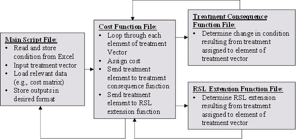
Figure 38. Flowchart. Basic algorithm for implementing MDSHA procedures in Matlab™.

Once the MDSHA approach was recreated and all models and data gathered, comparisons were made between the outputs of the RSI implementation and the outputs supplied by MDSHA. The purpose of these comparisons was to ensure that the MDSHA process was replicated and that all models and costs implemented in the RSI validation code developed by the project team matched the outputs supplied by MDSHA. A subset of pavement sections were randomly selected to verify the implementation of the MDSHA process.

Three types of verifications were conducted to test the agreement between the RSI implementation and the MDSHA results. The first verification was to check that the condition of pavement sections over time matched the information provided by MDSHA for pavements that had no treatment applied. An example of this first verification is shown in table 17 for a sample pavement section, where it can be seen that the Matlab™ RSI implementation matched the values provided by MDSHA. This agreement was consistent in all pavement section samples checked.

The second level of verification was to compare the cost and resulting condition of applying a treatment to a pavement section at a given point in time to the results provided by MDSHA. This verification was performed over many pavement sections, and, similar to the first verification, the values produced by the Matlab™ RSI implementation consistently matched the values provided by MDSHA. An example of this type of verification is shown in table 18, where micro-surfacing applied in 2017 was shown to be the optimal treatment.

The third verification involved performing a treatment selection, in terms of both treatment type and timing, by maximizing the objective function in figure 37 and comparing the treatment selection to the optimization results provided by MDSHA. This verification was performed following a revision of the algorithm shown in figure 38 to include an optimization component. Similar to the first two verifications, the results produced by the Matlab™ RSI implementation matched the data provided by MDSHA. For example, the pavement section shown in table 18 was evaluated using the Matlab™ RSI algorithm, and the algorithm also chose micro-surfacing applied in year 2017 as the optimal treatment. This follows the results obtained from MDSHA.

Implementing MDSHA Data and Models into the RSI Algorithm

Following the implementation and initial verification of the MDSHA approach, the algorithm presented in figure 38 was modified to implement the RSI approach. The modified algorithm incorporated an optimization routine prior to the cost function and reformatted the main script into a function that revised the output of the optimization so that it can be directly used by the remainder of the algorithm. The revision to the algorithm did not affect the MDSHA models and costs that were previously implemented and verified. The revised algorithm that demonstrates the inclusion of the optimization component and the removal of the RSL module is shown in figure 39.

 

Figure 39. Flowchart. Revised Matlab™ algorithm to include optimization.

In keeping with the approach of the RSI, the objective function presented in figure 37 was no longer used beyond testing the agreement between the Matlab™ RSI implementation and the results provided by MDSHA. Instead, the objective function was changed simply to minimizing total lifecycle costs over the chosen time horizon subject to condition thresholds. The revised objective function is shown in figure 40.

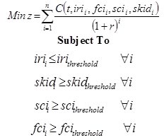
Figure 40. Equation. Objective function used in RSI validation.

Where:

z = The objective function value.
C = The treatment cost.
t = The treatment type.
i = The index year.
r = The discount rate (taken as 3 percent).
n = The number of years in the evaluation.

The threshold values for each condition measure, which appear in the constraints, were defined as the value for each measure that corresponded to zero remaining life as defined by MDSHA. It should be noted that while computing LCC, the RSI algorithm did not use the remaining value of the pavement section at the end of the analysis period, a limitation that required a long enough analysis period to minimize its effect on LCC comparisons.

Optimization Procedure

The problem construct as shown in figure 40 is discrete, nonconvex, and non-differentiable, all of which are properties required for exact solution methods. In addition, the size of the solution space is too large to conduct a comprehensive search for the optimal strategy. Generally, the solution to choosing the optimal M&R strategy can be viewed as an optimal path problem, and the optimization problem can be constructed based on dynamic programming, which is a method of breaking each problem into several sub-problems that are optimized and then recursively stepping through the problem. However, in the case of this problem construct, the number of feasible paths is very large. Removing constraints (e.g., not defining a minimum time between treatments) results in 16ⁿ possible permutations, where n is the number of years chosen. In other words, if a 60-year time horizon is evaluated, the number of possible permutations is approximately 1.8*10⁷². The number of feasible paths can be reduced by implementing rules, such as specifying a minimum number of years between treatments, but a goal of this research was to limit the number of constraints placed on the optimization in order to consider the entire feasible solution space. Therefore, a dynamic programming construct was not considered feasible.

The application of optimization techniques to solve pavement strategy selection has been widely reported in literature. However, the optimization is generally limited to determining the time to place a single treatment or, as is discussed in Sathaye and Madanat, selecting the treatments with the timing defined by thresholds.⁽⁴⁷⁾ Medury and Madanat present approaches for selecting strategies using Markov decision processes as a two-stage bottom-up approach using discrete state transitions for performance prediction.^(48–50) However, implementing the approach in Medury and Madanat would require significant modifications (e.g., implementing Markov deterioration models) to the models provided by MDSHA, which was not desirable for the RSI validation effort.⁽⁴⁹⁾

Given the construct of the problem, as well as the size of the solution space, it was decided that genetic algorithms were the most promising technique to determine optimal treatment strategies. Genetic algorithms are techniques to solve combinatorial optimization problems in the family of evolutionary algorithms, which are based on the Darwinian concept of survival of the fittest.⁽⁵⁰⁾ In genetic algorithms, a combination of values are treated like a chromosome in biology, and the fitness of the chromosomes are evaluated using a fitness function. In the case of this research, chromosomes are a string of numbers representing a given treatment in a given year (e.g., the value of 1 in the fifth position represents do nothing in year 5). The fitness function is the value of the objective function shown in figure 38, and a comparison is made between the chromosomes on the basis of a scaled value of the fitness function. On this project, a rank scaling was used, meaning that the values of the fitness function were ordered from most to least desirable and then assigned a numerical ranking to represent desirability.

The basic concept of genetic algorithms is to mimic evolution to determine the input values of an objective function that produce highly fit outputs. The general approach to the evolution of the solution in genetic algorithms is shown in figure 41. Conceptually, the parent population represents a series of highly fit solutions, and these solutions are then sent through operators that are designed to mimic evolutionary theory to generate a set of offspring. In essence, on this project, the genetic algorithm is used to generate new sets of future streams of pavement improvements at different times that are evaluated against the objective function. The genetic algorithm has the following three main operators as discussed in Surajudeen-Bakinde et al.⁽⁵¹⁾:

1. Stochastic selection: Some “elite” parents are chosen for survival to the next generation, and other survivors are chosen with probability based on the scaled value of the fitness function. This ensures some suboptimal survivors exist so that a level of diversity continues throughout generations.
   
   
2. Scattered crossover: Two parents are chosen to mate, and then a crossover point is randomly chosen so that the next generation is a combination of attributes of the parent generation.
   
   
3. Mutation: Some members of the parent generation are randomly mutated to form the next generation. This random mutation ensures diversity in the population so that the algorithm is less likely to remain stuck in a localized optimum.

 

Figure 41. Graphic. Basic flow of chromosomes in the genetic algorithm.

The genetic algorithm procedure was implemented in Matlab™, and the Global Optimization toolbox was selected as the main optimization environment for the RSI validation. The Matlab™ implementation of genetic algorithms was selected because it provided the readily available framework of the genetic algorithm while also allowing the user to manipulate the settings (e.g., mutation rates, fitness scaling, etc.).

The function minimized by the genetic algorithm was the discounted present value of the cost objective function in figure 40. The problem was constructed using integer constraints, and the input to the objective function was a vector of treatments, which is represented as the values of t in figure 40. The vector of treatments was constructed such that a value of one represented the do-nothing condition, and then integers were assigned to each treatment. The location of the number within the vector represented the year that the treatment was applied. For example, the vector [1 1 1 5] is representative of no M&R for the first 3 years and a thin overlay applied in year 4. This vector is what the genetic algorithm manipulated to find solutions for the objective function in figure 40.

The constraints shown in figure 40 were set up as penalty values for the value of the objective function. The condition metrics (IRI, skid number, SCI, and FCI) were evaluated at each step in time, and if the constraints were violated, the treatment cost was assigned a cost of 10⁶, which is much higher than any expected treatment cost for the pavement. The penalty value was evaluated during the development of the optimization procedure, and it was found that the value of the penalty had a strong influence on whether the optimization reported local optimums or converged to a global optimum. Higher values for the penalty resulted in more local optimums reported. This is because larger differences in fitness function values result in a lower probability that the parent associated with the worse fitness score will be carried on through future generations. In other words, once a local optimum is discovered, the genetic algorithm converges on it much more rapidly for higher values of the penalty assigned for violating the constraints.

The initial population input into a genetic algorithm is an important parameter because it has an effect on computational efficiency and the convergence towards a globally optimal solution.⁽⁵²⁾ Essentially, there is a tradeoff between computational time and the ability of the algorithm to consistently converge on the same optimal value. In order to address this, several trials were conducted in order to determine how to best construct the initial population. These trials consisted of varying the size and characteristics of the initial population and running several loops of the same optimization in order to determine which set of characteristics of the initial population led to the fewest variations in solutions. The final selection of the initial population was set so that each optimization had a mixture of standard initial inputs and random initial inputs.

The genetic algorithm procedure implemented in Matlab™ allows for the following two options when generating an initial population for the optimization:

• A randomly developed initial population.
  
  
• A user-specified initial population.

For this project, it was determined that the best initial population consisted of mixing the two options. A total of 62 strategies were developed that represented possible optimal solutions for various permutations of initial pavement conditions. For example, it was conjectured that a pavement with very high age, high IRI, and high cracking would best be suited by a strategy calling for reconstruction in the first year followed by preservation in 8-year intervals. Although this may be a reasonable strategy, it may not be always an optimal strategy for all pavements with a poor initial pavement condition. The genetic algorithm uses the initial strategies in the initial parent generation to create future combination of treatments to be evaluated that trend toward a more optimal combination of treatments. In addition, it was expected that the optimal strategy for any given pavement will include more values equal to one (do nothing) than values that are greater than one. This was specified in the initial population. Finally, 38 random strategies were specified to be created by Matlab™, and the random strategies changed in every iteration of the optimization.

Given the stochastic nature of the genetic algorithm, optimality cannot be guaranteed. However, several steps can be taken to promote certainty that a global optimal solution is found. One characteristic of the optimization problem that affects whether the genetic algorithm converges on local optimums or the global optimum is the topography of the solution space. In other words, the change in the fitness function values for each potential solution affects whether the final solution is more likely to be a global optimal or a local optimal. To illustrate this, two potential representations of the solution space topography are shown in figure 42. The topography represented in figure 42a contains clear minima that are consistent, and the topography represented in figure 42b contains minima hidden in a considerable amount of noise. Given that global optimization can be viewed as a hill climbing problem where the topography of the solution space effects the response of the algorithm, the solution space represented in figure 42a is more conducive to a genetic algorithm more consistently finding the global optimization, assuming that an adequate population is specified to spread across the solution space. It is expected that by treating the constraints as a penalty on the cost and making the penalty consistent (i.e., not dependent on the characteristics of the pavement), the solution space of the optimization in the RSI validation is more closely represented by figure 42a.

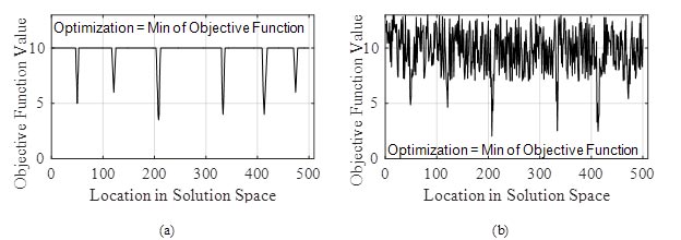
Figure 42. Graphs. Comparison of solution space topographies with different complexity.

Another approach to ensuring that a global optimum is reached is to add diversity into the population once the algorithm begins to converge on a solution. The added diversity causes the population to expand across the solution space. Instead of using functions within the genetic algorithm toolbox in Matlab™ to perform this, the algorithm used for this project was modified to add diversity at specified times and also to incorporate principles of another global optimization procedure known as simulated annealing. Simulated annealing is an optimization procedure designed to mimic the metallurgical process of annealing by essentially starting with a large number of potential solutions and then randomly perturbing the solutions and selecting a certain number to carry through to next steps with some changes.⁽⁵³⁾ The criteria that specifies whether a solution is carried forward in simulated annealing is defined by an acceptance probability function, and the number of solutions carried forward decreases over time. The acceptance probability function places a higher probability that more desirable states are carried through the solution but also maintains a probability that some less desirable states survive to maintain diversity. Essentially, in the first steps, the potential solution space is searched broadly, and then, as specific potential solutions are identified, the population carried forward is forced to reduce toward optimums within the solution space.

Using the basic principle of simulated annealing, as well as the concept of added diversity in genetic algorithms, three levels of loops were set up to solve the genetic algorithm in this project. In the first level, the initial population was large (100 streams of alternative improvement scenarios (chromosomes) consisting of 62 specified and 38 random), and the stopping criteria was less strict (i.e., the relative change in the fitness function was allowed to be higher than the final level). This level was solved through eight loops, and the solutions were stored. The solutions to the first eight loops were used to create a new population by manipulating these first solutions. The manipulations included shifting the chromosomes and artificially adding values of one in place of treatments. Upon studying several solutions from the first level of the algorithm, it was found that several treatments were more optimal if they were shifted in time (e.g., a micro-surfacing is more optimal in year 5, but the algorithm recommended it in year 4). This is indicative of the algorithm becoming stuck in local optimums, and thus, the manipulations were designed to address this shift in time.

The second level included the manipulated solutions from the first level as well as several randomly generated solutions to create a smaller initial population (on average between 50 and 60). The second level was looped three times and the solutions stored. Finally, the third level included manipulating the solutions in the second loop and adding some random diversity to create a much smaller initial population (approximately 20), and the genetic algorithm was run once more with more strict stopping criteria than the first two levels. Although this overall process was very computationally intensive, it produced results that were consistent and provided higher assurance that the globally optimal solution was identified.

Problem Construct

Once the genetic algorithm was calibrated to produce consistent solutions that were expected to be the globally optimal solutions, the MDSHA data were incorporated into the algorithm. Only asphalt pavements were considered in this analysis, although the algorithm could be easily modified to consider rigid and composite pavements. Asphalt pavements represent the majority of pavement sections in the MDSHA network. This section of the chapter presents the methods used to select the sample of pavements, the method for using cloud computing applications to solve the RSI optimization, and the analysis period for the LCCs.

Sample Selection

From analyzing the MDSHA optimization results, their analysis was performed on 3,082 unique segments. Of these segments, 204 were already scheduled for work before 2017 (i.e., these are not in the optimization). Of the remaining 2,878 unique segments used in the optimization, 1,716 were identified as flexible pavements, and 1,653 of the flexible sites had complete 2014 datasets. After evaluating the required computational costs of performing a 40-year strategy selection optimization on each of the 1,653 segments, it was determined that although it was possible to analyze all segments, the best approach would be to select a representative sample from the 1,653 segments on which to perform the optimization.

In order to determine whether a sample could be selected so that it represented the MDSHA flexible pavement network, an optimization algorithm was devised so that the objective was to minimize the number of sites selected given some constraints. The constraints were based on the results of the two-sample Kolmogorov-Smirnov test, which is a nonparametric test used to compare two distributions. Thus, it was chosen to compare the selected sample to the initial population. Eight factors were chosen to describe the characteristics of the network: district, functional class, AADT, IRI, initial FCI, initial SCI, initial rutting, and initial skid number values. The constraints were set up so that when the selected subset was compared to the initial population, the results of the two-sample Kolmogorov-Smirnov test (with an α of 0.01) indicated that the null hypothesis of the two samples coming from the same distribution could not be rejected. Finally, it should be noted that any covariance between the selected characteristics was neglected for the sake of this sampling. However, a level of correlation does exist between the characteristics (e.g., a higher initial functional cracking is likely to also correspond to a higher initial structural cracking).

The results indicated that the network could be adequately represented using 338 unique pavement sections. The cumulative histograms were compared for the sample of 338 and the initial population of 1,653, and the results are shown in figure 43. It can be concluded from this figure that the selected sample is representative of the larger population and that only 338 segments are required to represent the initial population.

 

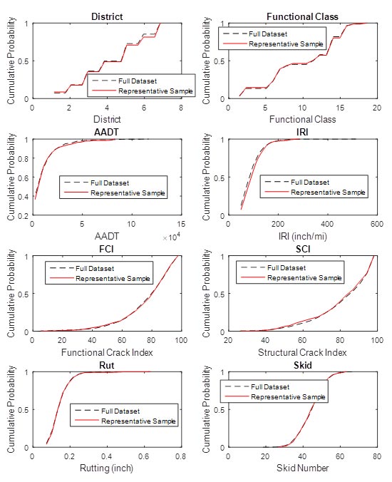
Figure 43. Graphs. Comparison of the sample set characteristics of the initial population to the chosen sample.

Cloud Computing Application

The genetic algorithm can be a very computationally intensive optimization approach, and the setup of the process as described earlier in this chapter increased the time required to converge to optimal solutions. Therefore, it was determined that solving the genetic algorithm for 338pavement sections over varying analysis periods was not feasible on a single computer. Instead, parallel computing strategies and cloud computing applications were required to solve the optimization within the project time constraints.

Parallel computing includes separating independent pieces of a calculation and sending the separate pieces to different processors within either the same or separate computers. Sending the parallel calculations to processors in separate computers is essentially the concept behind cloud computing. For example, it was described earlier how several loops were incorporated into the optimization algorithm, and each of the loops within a single level are independent of each other. Thus, each of these loops can be run in parallel on separate processors.

In order to apply these concepts to the RSI validation effort, the Parallel Computing toolbox in Matlab™ was incorporated into the algorithm. The parallel processes were sent to virtual workers in the Amazon Web Services® environment, and the solutions were returned and stored on a local computer. It was found that by using the cloud computing applications, the time required to develop optimal solutions was decreased by a ratio of approximately 15:1.

Analysis Period Selection

In order to assess the effect of the time horizon on the optimal strategy selection, the optimization analysis period (n in figure 40) was set to 20, 40, and 60 years. Given the specific objective function (minimizing lifecycle costs without including remaining value), the effect of the analysis period can be significant depending on the specific characteristics of the pavement network (e.g., deterioration rate). It is important to note that it is expected that the effect of the analysis period would be mitigated if a salvage value is applied at the end of the analysis period. For example, the objective function in figure 40 dictates that the most optimal solution is not to apply a treatment if the constraints are not violated. If a salvage value was applied (e.g., as a negative cost in the objective function), then a lowest lifecycle cost alternative would be expected to result in a better condition at the end of the analysis period. In the case of the objective function used in this validation, a short analysis period would result in no treatment applied to a significant portion of the pavement network and a worsening of the average pavement condition toward the end of the analysis period.

Once the optimization was completed for all three analysis periods, the resulting average network condition was compared. The average network roughness for all three analysis periods is shown in figure 44, the average network SCI is shown in figure 45, and the average network FCI is shown in figure 46 as a function of time. Several significant trends emerged when comparing the analysis periods, and these can be seen in figure 44 through figure 46. First, in each case, the first 10 years of the analysis produced relatively consistent results. This time period is heavily influenced by the initial condition of the pavement network, and some of the constraints required early treatments selection based on the initial condition. For example, micro-surfacing was not allowed on very poor pavements (based on the models and business rules supplied by MDSHA), and thus, the initial conditions of the network dictated which pavements could be selected for micro-surfacing.

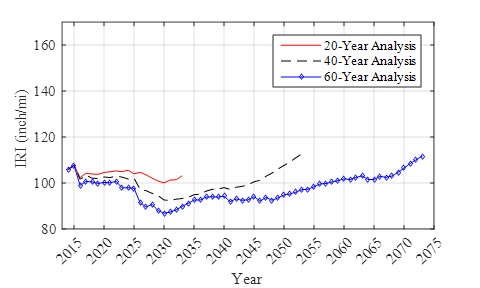
Figure 44. Graph. Average network roughness for three analysis periods.

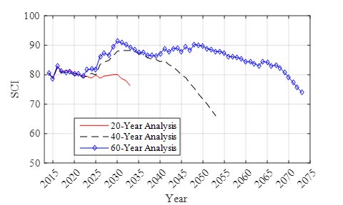
Figure 45. Graph. Average network SCI for three analysis periods.

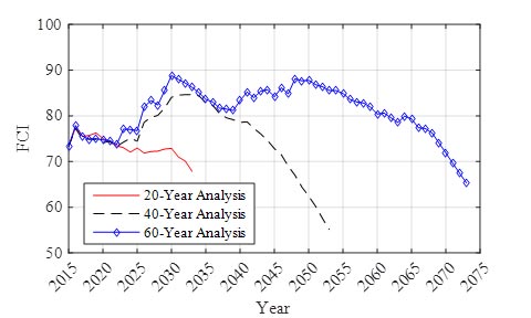
Figure 46. Graph. Average network FCI for three analysis periods.

Another observation to be made from the trends seen in figure 44 through figure 46 is that there is a time horizon when the pavement condition begins to deteriorate. This occurs approximately during the last 20 years for the 40- and 60-year analysis period. This time horizon is driven by the objective function, and in the case of this validation, a salvage value was not included in the lifecycle cost calculations. As described earlier, the lowest cost option is to do nothing as long as the constraints are not violated, and thus, pavements that were maintained in good condition over the initial portion of the analysis period will be allowed to deteriorate over the latter portion.

There is a time period when the pavement condition is stable and consistently maintained in good condition. This occurs at between 2030 and 2035 in the 40-year analysis and between 2030 and 2050 in the 60-year analysis. It has been proposed in pavement management that the lowest costs are realized when the pavement network is maintained and preserved in good overall condition, and this stable time period appears to support this hypothesis.

Based on the comparisons between the three time horizons, it was determined that the RSI validation effort would be conducted using the first 20 years of the 40-year analysis. By selecting the first 20 years of the 40-year analysis, the effect of the length of the analysis period on the optimization results was minimized while also including a significant time frame for comparisons. In addition, this was selected because the comparison against the MDSHA results are limited to only the first six years of the analysis period.

RESULTS

The results of the RSI implementation were compared to the results from the MDSHA analysis in terms of the yearly costs, work type, and condition metrics (IRI, SCI, FCI, and skid number). Although the time horizon and objective functions from the two approaches are different (see figure 37 and figure 40), it is expected that if the RSI methodology represented a valid approach, then the RSI methodology would lead to consistent prediction of treatment needs, performance, and costs over the analysis period. Finally, it is important to note that the results are comparing optimal strategies for each pavement section (i.e., an unconstrained analysis), which is the first step in a bottom-up network optimization approach. The next step in a network-level optimization would be to select the pavement sections that would receive work in a given year to address budget constraints, and this optimization would be performed on a yearly basis.

When comparing the yearly costs (figure 47), the same trend was seen for the first 3 years, with the large costs in the first year representing the accumulated backlog. Recall that the work for 2015 and 2016 had already been scheduled, and, thus, the optimization begins in 2017 using the 2014 condition data. The 2018 cost from the RSI validation is very low (approximately $25,000 USD), and the costs begin to stabilize in 2019. The 2020 costs from the MDSHA approach are very high and include many sites in which the optimal choice would be to defer M&R activity past 2020. However, the form of the MDSHA objective function (see figure 37) dictates that practically every pavement section will have work recommended within the specified time horizon, which was 6 years (2015 to 2020) according to the MDSHA data. It is important to note that the MDSHA optimization approach is a biennial process, and the last 2 years of the optimization are not scheduled for work. In other words, a 6-year time horizon is evaluated in order to develop treatment schedules for the third and fourth years.

 

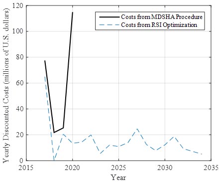
Figure 47. Graph. Comparison of yearly M&R costs.

For both RSI and MDSHA procedures, the mix of identified work types—do nothing, preservation, and rehabilitation—were compared (in figure 48 to figure 50), and in both procedures, much more work was recommended in 2017 than in either 2018 or 2019. It was found that the treatments in 2017 are heavily dictated by the 2014 condition irrespective of the optimization procedure. In other words, the treatments that can be selected for given pavement sections are constrained by the initial condition. There was very little agreement in the 2018 through 2020 mix of work types for preservation (figure 49) and rehabilitation (figure 50) (although the trends were similar for years 2017 through 2019). The MDSHA procedure did not recommend reconstruction, and the RSI validation approach had 9-percent reconstruction in 2017 and 13-percent reconstruction in 2020.

 

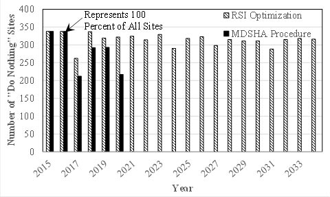
Figure 48. Graph. Recommended do nothing sites per year.

 

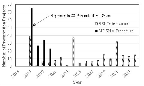
Figure 49. Graph. Recommended preservation work per year.

 

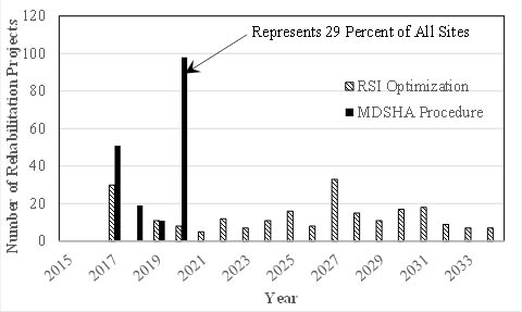
Figure 50. Graph. Recommended rehabilitation work per year.

The resulting condition based on the MDSHA procedure and the RSI process was compared in terms of IRI, FCI, SCI, and skid number in figure 51 to figure 54. Similar to the yearly costs presented in figure 47, the MDSHA process resulted in a significant improvement in the measures in year 2020, which is a result of the specific objective function used to select treatments. The MDSHA process results in a slightly better condition in each case. However, in the long term (approximately 15 years), each measure resulting from the RSI optimization matched the 2019 values from the MDSHA process. In other words, the RSI optimization procedure leads to a consistent prediction of treatment needs, performance, and costs over the analysis period.

 

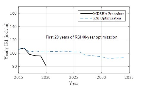
Figure 51. Graph. Average network roughness resulting from MDSHA and RSI approaches.

 

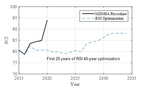
Figure 52. Graph. Average SCI resulting from MDSHA and RSI approaches.

 

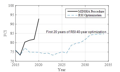
Figure 53. Graph. Average FCI resulting from MDSHA and RSI approaches.

 

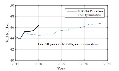
Figure 54. Graph. Average skid number resulting from MDSHA and RSI approaches.

The average pavement roughness resulting from both the RSI and MDSHA approaches is shown in figure 51. For the RSI optimization, it can be seen that the roughness remained relatively steady over the first 11 years and then began to decrease steadily over time. This relatively steady time frame of approximately 10 years was present in each condition metric and was also present in the three time horizons evaluated (20, 40, and 60 years). The SCI (figure 52), FCI (figure 53), and skid number (figure 54) demonstrated the same behavior as the roughness. It should be noted that an improvement in the skid number, FCI, and SCI is demonstrated by an increasing value, whereas an improvement in roughness is signified by a decrease in the value.

Figure 55 through figure 57 show the IRI, SCI, and FCI, respectively, at the time of preservation for both the MDSHA and RSI approaches. Any work recommended in 2020 for the MDSHA approach was not included in these figures given that the time horizon (6 years) used in the MDSHA approach significantly affected the 2020 results as discussed earlier. For each measure, preservation is recommended when the pavement is in better condition for the RSI optimization than for the MDSHA procedure. According to the MDSHA data provided, two sites were exempted from the constraints for the preservation treatment set at IRI threshold of 170 inches/mi by MDSHA models. However, the RSI optimization placed constraints on the condition ranges for which preservation was allowed (based on MDSHA provided models).

 

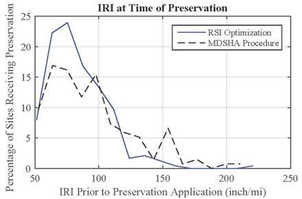
Figure 55. Histogram. Pavement roughness at time of preservation.

 

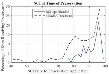
Figure 56. Histogram. SCI at time of preservation.

 

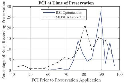
Figure 57. Histogram. FCI at time of preservation.

Figure 58 through figure 60 show the IRI, SCI, and FCI, respectively, at the time of rehabilitation for both the MDSHA and RSI approaches. Contrary to the findings of the average condition when preservation was recommended, the average value for each measure when rehabilitation was recommended represented worse pavement condition for the RSI optimization than for the MDSHA procedure. In other words, the RSI optimization generally recommended that preservation be applied on pavements in better condition, and rehabilitation applied on pavements in worse condition than the MDSHA procedure. This is an expected outcome given that the FCI and SCI were the two measures that mostly triggered M&R, and rehabilitation effectively resets the FCI and SCI values back to 100 irrespective of the initial pavement condition.

 

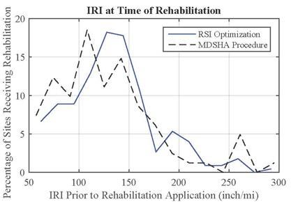
Figure 58. Histogram. Pavement roughness at time of rehabilitation.

 

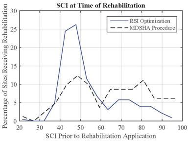
Figure 59. Histogram. SCI at time of rehabilitation.

 

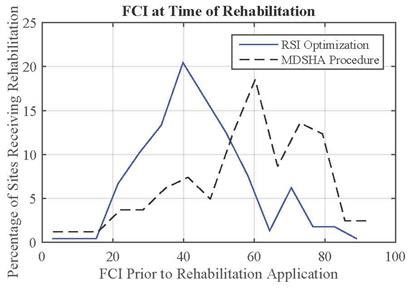
Figure 60. Histogram. FCI at time of rehabilitation.

Linking the MDSHA PMS Process and RSI Concept

The RSI concept is based on the idea that pavement’s M&R requirements cannot be defined by a single value representing the end of life of the pavement. Instead, pavements should be described based on intervals used to communicate the amount of time before a treatment type is required to provide acceptable or above acceptable LOS at the lowest practical LCC. Implicit in this change in terminology is the idea that describing a pavement using service intervals more closely reflects how pavements are maintained (i.e., not all pavements are allowed to reach terminal serviceability). Also implicit in this change in terminology is that a given pavement can be described using a string of information that represents an optimal treatment sequence and timing.

To demonstrate the differences, the remaining life information for each of the 338 pavement sections used in the optimization was obtained from MDSHA data and compared to the timing until first treatment from the RSI optimization. In this case, the first 40 years of the 60-year analysis was used because a portion of sites had no work recommended in the first 20 years of the 40-year analysis. Pavements with no work recommended in the first 20 years of the 40-year analysis were generally newer pavements on routes that have low rates of deterioration and relatively high condition thresholds. For example, nine pavements in relatively good initial condition (IRI < 100 inches/mi, FCI > 80, and SCI > 85) in functional class 6 (IRI threshold of 250 inches/mi, FCI threshold of 30, and SCI threshold of 45) had no work recommended in the first 20 years of the 40-year analysis. Incidentally, many of these pavements had preservation recommended within the first 40 years of the 60-year analysis.

Any pavements with no treatment recommended in the first 40 years were placed in the 45-year bin. The results are shown in figure 61, and it can be seen that the optimal decision generally results in the first treatment being placed before the remaining life is reached on average. It should be noted that the RSL computes the time until the pavement reaches a predefined terminal condition, while RSI computes the time until any treatment is applied. In addition, figure 62 demonstrates that practically no relationship exists between the time until the first pavement treatment from the RSI optimization and the remaining life information obtained from MDSHA.

 

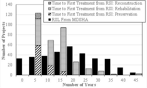
Figure 61. Graph. Remaining life (MDSHA) compared to time until first treatment from RSI.

 

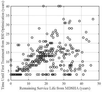
Figure 62. Graph. Time until first treatment from RSI as a function of remaining life.

More fundamentally, RSI defines specific intervals until certain M&R activities should be performed on a pavement. As demonstrated throughout this chapter, the intervals can be developed using optimization based on minimizing lifecycle costs. To demonstrate how the final RSI intervals look after the optimization, a sample of segments are demonstrated in table 19. The RSI columns in table 19 contain the number of years relative to 2014 that the actions should be undertaken.

Discussion

Validating the RSI using the MDSHA models successfully demonstrated that the RSI concept can be implemented at a State transportation department with minimal changes to the condition metrics, performance models, and other information. However, implementing the RSI requires a long-term outlook for the treatment selection process in order for the optimization to provide adequate information. For example, implementing the objective function presented in figure 40 (minimizing costs subject to condition thresholds) in MDSHA’s typical 6-year outlook would result in the majority of pavement sections requiring no maintenance and would also lead to the eventual long-term decline in network condition. Instead, it was demonstrated that the time horizon for the analysis should be based on the deterioration characteristics of the pavement (e.g., rate of deterioration) and should also be based on the characteristics of the objective function in the optimization.

Although the validation effort presented in this chapter resulted in several insights into pavement management practices, it is important to recognize several key differences in the two procedures that were compared. The differences are summarized in table 20.

The objective function is a mathematical expression of the agencies’ preferences and determines the results of the optimization. For example, the MDSHA objective function (figure 37) explicitly includes a measure of benefit in the numerator, and the results of the optimization indicated that it leads to a much more aggressive approach toward improving network condition than the lowest lifecycle agency cost objective function used in the RSI validation (figure 40). However, it is important to note that the MDSHA approach is not designed to select treatments over the 6-year time frame. Instead, the MDSHA approach is to evaluate a 6-year horizon but use the results from years 3 and 4 to select optimal strategies. In addition, there is no explicit measure of benefit in the objective function used for the RSI validation. Instead, the benefit in the RSI validation is implicit; if managing a network in good condition results in overall lower costs, then the network condition will improve over a long enough time horizon.

Although the results of optimization are almost entirely dependent on the objective function that is developed to express the goals of the analysis, the comparison of the MDSHA procedure and the RSI optimization approach yields many findings. In every case, the MDSHA procedure resulted in higher annual costs and better overall condition earlier in the time horizon. This tradeoff between M&R costs and condition is expected, and the differences between the MDSHA and RSI approaches are a result of the differences in the objective functions used to perform the optimization.

MDSHA has developed models to account for the improvement in condition due to a treatment as a function of the initial treatment condition. The RSI formulation developed for this project would not have been possible without the use of the MDSHA models, business rules, condition data, and cost data. For example, rehabilitating a pavement with a lower IRI results in a smoother pavement than rehabilitating a pavement with a higher IRI (though the same does not hold true for the FCI and SCI) using the MDSHA models. In addition, several performance models were related to the last treatment applied (e.g., the pavement roughness grew at a slower rate after the application of micro-surfacing), and several costs were a function of the pavement condition. These relationships had a direct impact on the optimal treatment schedules developed during the optimization and led to preservation being recommended when the pavement was in a better condition. Absent these models (i.e., if the effect of a treatment (posttreatment performance) did not depend on the pretreatment condition), more preservation would be recommended later in the pavement life simply because of the costs being discounted over time.

Finally, the optimization algorithm used in this validation is computationally intensive; the resources required to converge on a solution are relatively high. However, the algorithm was not designed to balance efficiency with robustness. Instead, the algorithm was designed to increase certainty of converging on the global optimum, as opposed to a local optimum. In addition, the use of cloud computing resulted in the ability to develop solutions for a relatively large number of pavements over a relatively short time. Additional work on the algorithm, such as better balancing the population size as the algorithm progresses or developing better methods to intelligently add diversity to the population, would undoubtedly reduce computational intensity.

It is clear that the following enhancements to MDSHA would make an already mature process even more efficient:

• Posttreatment improvement in pavement condition and performance are affected by the pretreatment pavement condition. Rehabilitation on pavements in better condition will yield better posttreatment condition than on pavements in poor condition. However, when rehabilitation treatment is applied, the FCI and SCI models currently reset to 100 percent irrespective of pretreatment condition, and these models should be improved.
  
  
• Performance prediction is typically based on the previous applied treatments and conditions. These factors can be used in improving the performance predictions instead of using only the age of the current treatment (see figure 34 through figure 36). The use of only treatment age will predefine the treatment performance irrespective of the pavement condition at the treatment time.
  
  
• The last treatment is used to predict future IRI performance, but the efficiency of the preservation treatments is dependent on the past rehab treatments that still provide a structural component to the pavement structure. A structural evaluation parameter is needed to account for overall pavement condition instead of considering only the last treatment.

Conclusions

The following conclusions were developed based on the analysis and results presented in this chapter:

• The implementation of the RSI approach can be accomplished with relatively few changes to agency models and data. In this validation effort, only the optimization method used in the treatment selection was modified, given the state of the models provided by MDSHA. Although this is a significant change from the perspective of network-level decision processes, no changes to data collection, performance models, or treatment selection criteria were attempted.
  
  
• In any decision analysis framework, agency goals are mapped to the decisionmaking process through the construct of the objective function. Consequently, the objective function and underlying assumptions used in the analysis have a significant impact on the long-term condition and projected yearly costs of the pavement network. Therefore, many key decisions, such as the analysis period, should be reflective of the objective function used in the analysis.
  
  
• In addition to being influenced by the objective function, the analysis period should be based on the performance characteristics of the pavement condition if minimization of costs is a goal in the optimization. For example, if a network of pavements generally deteriorates at a relatively lower rate, the time horizon should be much longer than a network of pavements that deteriorates at a higher rate. This is because the analysis period should cover enough time for multiple treatments to be required for given pavement sections.
  
  
• If the construct of the objective function is to minimize costs subject to condition thresholds, then a significant portion of time at the end of the analysis period should be neglected when the end of analysis period remaining value is not considered. This is because the optimal solution will generally be to maintain a pavement in good condition until such a time that, when do-nothing is selected for the remainder of the pavement life, the pavement does not require maintenance. For example, if a 40-year analysis period is selected and it takes 20 years for a good pavement to reach the condition thresholds, the optimal solution will be to maintain the pavement in good condition for the first 20 to
  25 years and then allow it to deteriorate toward the thresholds.
  
  
• Although the optimization algorithm presented in this report is computationally intensive, parallel computing using cloud resources provides an economical means for addressing large network optimization issues. Computational resources should no longer be viewed as a constraint in optimization.

Recommendations

The following general recommendations are based on the results of this validation process:

• The RSI concept should be pursued and implemented by agencies in an effort to enhance their decision processes as well as improve how M&R needs for pavements are effectively communicated to stakeholders at all levels.
  
  
• More research is needed to better understand the tradeoff between computational intensity and solution robustness when using genetic algorithms to perform optimization specific to pavements. This research may help decrease the computational resources required for using the genetic algorithm as a strategy selection technique over long-
  term horizons.
  
  
• Hard constraints were used for the optimization in this chapter. Essentially, if the condition fell below a specified value, then the costs were severely penalized. However, more optimal solutions may be found if these constraints are softened, which can be done using a goal programming type of approach. Future optimization procedures that maintain a focus on minimizing costs subject to condition thresholds should consider evaluating the use of these soft constraints instead of the use of hard constraints.

⁵ Nathan Moore, email message to author, October 6, 2015.

⁶ Moore, op. cit.

⁷ Moore, op. cit.

⁸ Moore, op. cit.