U.S. Department of Transportation
Federal Highway Administration
1200 New Jersey Avenue, SE
Washington, DC 20590
202-366-4000
Federal Highway Administration Research and Technology
Coordinating, Developing, and Delivering Highway Transportation Innovations
| REPORT |
| This report is an archived publication and may contain dated technical, contact, and link information |
|
| Publication Number: FHWA-HRT-13-066 Date: August 2013 |
Publication Number: FHWA-HRT-13-066 Date: August 2013 |
The load test results from GRS performance testing have been used in the design of GRS abutments. Designers can use the empirical results to estimate capacity (strength limit) and deformation (service limit) of the GRS abutment, needed in the internal stability design.(1) In addition, the database of results can be used to validate the GRS capacity equation (figure 8) and calibrate a more accurate LRFD resistance factor.
The results indicate that, based on the current limitations set forward by FHWA for GRS abutments of a 4,000-psf service pressure and a 0.5-percent vertical deformation service limit, seven GRS composites tested in this study may meet the strength and service limits (table 22).(1) The service limit pressure at a vertical strain of 0.5 percent is for the dead load only since live loads have not been found to impact the total strain for in-service GRS-IBS structures.(5) Note that only three GRS composites tested in this study meet both the design limits and the material specifications (Tƒ≥4,800 lb/ft, dmax ≥½ inches); however, based on the results of this study, consideration should perhaps be given to amend the criteria in future design guidance.
Table 22. PTs meeting GRS strength and service limit design criteria.
Test |
GRS Composite |
Design Strength Limit |
Service Limit |
|||||
ASD |
LRFD |
|||||||
Φ |
dmax |
Sv |
Tf |
|
q@ε=5% |
Фcap |
q@ε=5% |
|
DC-1 |
54 |
½ |
7⅝ |
4,800 |
19,983 |
5,709 |
8,992 |
3,065 |
DC-2 |
46 |
¾ |
7⅝ |
4,800 |
19,399 |
5,543 |
8,730 |
2,171 |
DC-4 |
49 |
1 |
7⅝ |
4,800 |
17,350 |
4,957 |
7,808 |
2,212 |
TF-2 |
53 |
⅜ |
7⅝ |
2,400 |
18,711 |
5,346 |
8,420 |
4,759 |
TF-6 |
53 |
½ |
7⅝ |
4,800 |
22,007 |
6,288 |
9,903 |
3,704 |
TF-12 |
53 |
½ |
3 13/16 |
1,400 |
18,573 |
5,307 |
8,358 |
4,028 |
TF-14 |
53 |
½ |
3 13/16 |
1,400 |
16,748 |
4,785 |
7,537 |
2,037 |
Φ = the peak friction angle, dmax = the maximum aggregate size, Sv = the reinforcement spacing, Tf = the MARV value of the wide width tensile strength,q@ε=5% = the stress at 5-percent vertical strain from a corresponding PT, FS = the factor of safety (equal to 3.5), Фcap = the resistance factor for capacity (equal to 0.45), q@ε=5% = the service stress at 0.5-percent vertical strain from a corresponding PT, ASD = Allowable Stress Design, and LRFD = load and resistance factor design.
PT results can be used to validate the ultimate capacity equation (figure 8). Figure 78 illustrates the comparison between the measured capacity from various PTs and the calculated capacity from figure 8. Note that figure 78 includes results from additional sources of research.(1,4 ,8,11 ,33 ,34) Based on the results of the PTs presented in this report and plotting the bias against the standard normal variable (figure 79 and table 23), the mean bias is 0.88 (i.e., the bias at a standard normal variable of zero) with a coefficient of variation (COV) of about 35 percent. Including other results from the literature, the average bias is 0.95 with a COV of about 32 percent (figure 80 and table 24).
The mean bias values near unity and low COV values for all of the GRS composite tests (table 24) indicate good agreement between the GRS capacity equation (figure 8) and the measured results. Note that the measured results used for comparison were taken at failure of the composite, not at a design limit of 5 percent vertical strain, as will be discussed later in the empirical method of design (see section 7.2.2). This may change the level of reliability between the analytical method and the empirical method of design, since both have equal factors of safety of 3.5. (1) A full LRFD calibration needs to be conducted to determine a more reliable resistance factor for each strength limit design method.
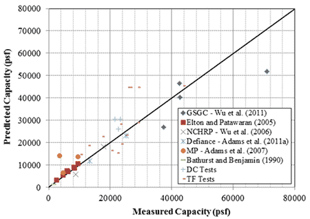
Figure 78. Graph. Comparison of predicted capacity and measured capacity.
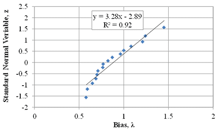
Figure 79. Graph. Cumulative distribution function plot for DC and TF PTs.
Table 23. Predicted and measured vertical capacity for DC and TF PTs.
Test |
Measured |
Predicted |
Bias, λ Measured |
Standard Normal Variable, z |
qult,emp |
qult,an,c |
|||
DC-1 |
23,310 |
30,439 |
0.77 |
-0.32 |
DC-2 |
22,709 |
25,952 |
0.88 |
0.16 |
DC-3 |
N/A |
40,812 |
N/A |
N/A |
DC-4 |
N/A |
17,078 |
N/A |
N/A |
DC-5 |
21,539 |
30,439 |
0.71 |
-0.49 |
TF-1 |
20,487 |
16,447 |
1.25 |
1.15 |
TF-2 |
25,260 |
23,403 |
1.08 |
0.67 |
TF-3 |
17,491 |
22,741 |
0.77 |
-0.16 |
TF-4 |
N/A |
44,786 |
N/A |
N/A |
TF-5 |
25,920 |
44,786 |
0.58 |
-1.56 |
TF-6 |
43,763 |
45,448 |
0.96 |
0.38 |
TF-7 |
26,546 |
44,786 |
0.59 |
-1.19 |
TF-8 |
29,134 |
44,786 |
0.65 |
-0.93 |
TF-9 |
22,310 |
15,369 |
1.45 |
1.56 |
TF-10 |
10,330 |
14,707 |
0.70 |
-0.54 |
TF-11 |
23,249 |
28,348 |
0.82 |
0.07 |
TF-12 |
29,030 |
29,001 |
1.00 |
0.54 |
TF-13 |
12,960 |
18,764 |
0.69 |
-0.72 |
TF-14 |
23,562 |
19,426 |
1.21 |
0.93 |
Mean Bias |
0.88 |
|||
Standard Deviation |
0.30 |
|||
Coefficient of Variation (percent) |
0.35 |
|||
N/A = Not applicable, did not fail the composite.
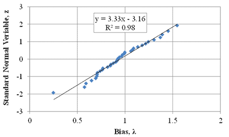
Figure 80. Graph. Cumulative distribution function plot for all GRS composite tests.
Table 24. Predicted and measured vertical capacity for all GRS composite tests.
Test |
Measured |
Predicted |
Bias, λ Measured |
Standard Normal Variable, |
Reference |
qult,emp |
qult,an,c |
||||
GSGC 2 |
70,957 |
51,841 |
1.37 |
1.24 |
11 |
GSGC 3 |
42,574 |
40,207 |
1.06 |
0.46 |
|
GSGC 4 |
37,252 |
26,795 |
1.39 |
1.40 |
|
GSGC 5 |
42,449 |
46,485 |
0.91 |
-0.10 |
|
Elton 1 |
4,805 |
5,324 |
0.90 |
-0.17 |
8 |
Elton 2 |
2,695 |
3,178 |
0.85 |
-0.31 |
|
Elton 3 |
6,392 |
6,909 |
0.93 |
0.03 |
|
Elton 4 |
6,100 |
7,226 |
0.84 |
-0.38 |
|
Elton 5 |
8,398 |
8,495 |
0.99 |
0.31 |
|
Elton 6 |
8,293 |
8,812 |
0.94 |
0.10 |
|
Elton 7 |
9,589 |
10,397 |
0.92 |
-0.03 |
|
NCHRP 1 |
8,356 |
5,685 |
1.54 |
1.93 |
33 |
NCHRP 2 |
17,757 |
18,287 |
0.97 |
0.24 |
|
Defiance 1 |
13,370 |
11,797 |
1.13 |
0.70 |
1 |
Defiance 2 |
25,068 |
23,030 |
1.09 |
0.61 |
|
Bathurst |
1,670 |
1,283 |
1.30 |
1.10 |
34 |
MP A |
4,696 |
6,371 |
0.74 |
-0.70 |
4 |
MP B |
3,548 |
14,044 |
0.25 |
-1.93 |
|
MP C |
9,600 |
13,493 |
0.71 |
-0.79 |
|
DC-1 |
23,310 |
30,439 |
0.77 |
-0.32 |
N/A |
DC-2 |
22,709 |
25,952 |
0.88 |
0.16 |
|
DC-5 |
21,539 |
30,439 |
0.71 |
-0.49 |
|
TF-1 |
20,487 |
16,447 |
1.25 |
1.15 |
|
TF-2 |
25,260 |
23,403 |
1.08 |
0.67 |
|
TF-3 |
17,491 |
22,741 |
0.77 |
-0.16 |
|
TF-5 |
25,920 |
44,786 |
 0.58 |
-1.56 |
|
TF-6 |
43,763 |
45,448 |
0.96 |
0.38 |
|
TF-7 |
26,546 |
44,786 |
0.59 |
-1.19 |
|
TF-8 |
29,134 |
44,786 |
0.65 |
-0.93 |
|
TF-9 |
22,310 |
15,369 |
1.45 |
1.56 |
|
TF-10 |
10,330 |
14,707 |
0.70 |
-0.54 |
|
TF-11 |
23,249 |
28,348 |
0.82 |
0.07 |
|
TF-12 |
29,030 |
29,001 |
1.00 |
0.54 |
|
TF-13 |
12,960 |
18,764 |
0.69 |
-0.72 |
|
TF-14 |
23,562 |
19,426 |
1.21 |
0.93 |
|
Mean Bias |
0.95 |
||||
Standard Deviation |
0.30 |
||||
Coefficient of Variation (percent) |
0.32 |
||||
N/A = not applicable, no reference number is associated with a test since results are
being reported for the first time in this report.
The strength design limit for capacity is defined as the stress at which the GRS composite fails (meaning it cannot sustain any additional load) or strains 5 percent vertically, whichever occurs first. To relate this to the ultimate capacity and to non-dimensionalize the results, the stress-strain curves were normalized by the ultimate capacity of the particular GRS composite for all of the PTs taken to failure (figure 81). The 5-percent vertical strain limit can significantly reduce the allowable stress placed on a GRS composite; figure 82 shows that at 5-percent strain, the applied pressure is between 50 and 85 percent of the measured ultimate capacity (table 8).
Along with the additional factor of safety of 3.5, using 5-percent vertical strain as a design strength limit for the empirical internal stability design is a conservative measure; however, it accounts for the resources available at most laboratory institutions so that PTs can be terminated at a reasonable, yet achievable, strain limit. The more important design limit for GRS walls and abutments is the service limit.
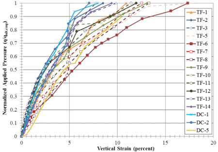
Figure 81. Graph. Normalized applied stress versus strain for all PT.
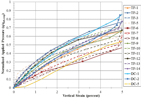
Figure 82. Graph. Normalized load-deformation behavior for the DC and TF PTs up to 5-percent vertical strain.
FHWA guidance currently recommends a service limit of 4,000 psf applied vertical stress (dead plus live load, with load factors = 1.0) with a target of 0.5-percent vertical strain for GRS abutments, measured by using only dead load, unless the engineer decides to permit additional load and/or deformation.(1) For a 20-ft-tall wall, the initial compression of the GRS composite would therefore be limited to 1.2 inches. Note that the majority of compression within a GRS abutment occurs shortly after placement of dead load, with little post-construction settlement, if constructed as outlined by FHWA.(5)
The stress-strain curve generated by the PT can immediately be used to estimate deformation. By knowing the applied dead load, the resulting strain can be found from the PT results. Alternatively, using a corresponding PT for the particular GRS composite would yield the amount of dead load (unfactored) that can be placed on the abutment to limit the deformation to the tolerable amount. For the range of tests conducted in this study (compacted only), the allowable applied stress is between 1,324 and 6,016 psf (table 8 and figure 84).
Using the normalized load test curves (figure 85), the service stress to meet the 0.5-percent vertical strain limit is 6 to 23 percent of the ultimate stress, with an average of 13 percent for all tests. For only the tests with a CMU facing, as would be typical in the field, the range is slightly narrower, between 8 and 19 percent with an average of 12 percent; for the tests without a facing element, the average is 15 percent.
When looking strictly at the PTs that meet the current FHWA specifications for a GRS abutment, the allowable applied stress at low strain levels (i.e., at in-service conditions) ranges between about 8 percent and 13 percent of the ultimate stress (figure 86), with an average of 10 percent. (1) By estimating an ultimate stress using the GRS capacity equation (figure 8), ignoring the effects of cohesion and confining stress as indicated by Adams et al. (2011a) for design of GRS abutments, and assuming 10 percent of the ultimate capacity, the maximum service stress (unfactored dead load only) to limit short-term vertical strain to 0.5 percent can be predicted (table 25).(1)
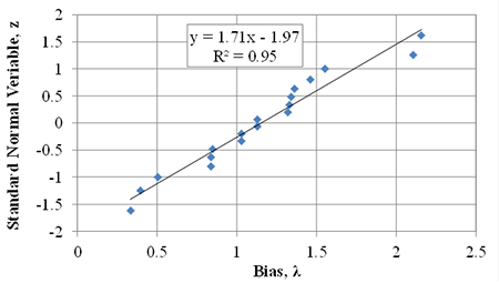
Figure 83. Graph. Cumulative distribution function for proposed service limit pressure.
Table 25. Estimation of allowable dead load to limit vertical strain to 0.5 percent using the GRS capacity equation.
Test |
Measured |
Predicted |
Bias, λ Measured |
Standard Normal Variable, z |
|
qult,emp(psf) |
q@ε=0.5 % (psf) |
q@ε=0.5 %, predicted = |
|||
DC-1 |
23,310 |
3,065 |
2,974 |
1.03 |
-0.34 |
DC-2 |
22,709 |
2,171 |
2,551 |
0.85 |
-0.48 |
DC-3 |
N/A |
1,324 |
4,021 |
0.33 |
-1.62 |
DC-4 |
N/A |
2,212 |
1,655 |
1.34 |
0.48 |
TF-1 |
20,471 |
2,068 |
1,570 |
1.32 |
0.20 |
TF-2 |
25,260 |
4,759 |
2,204 |
2.16 |
1.62 |
TF-3 |
17,491 |
3,417 |
2,204 |
1.55 |
1.00 |
TF-4 |
N/A |
3,705 |
4,409 |
0.84 |
-0.80 |
TF-5 |
25,920 |
6,016 |
4,409 |
1.36 |
0.63 |
TF-6 |
43,763 |
3,704 |
4,409 |
0.84 |
-0.63 |
TF-7 |
26,546 |
2,224 |
4,409 |
0.50 |
-1.00 |
TF-8 |
29,134 |
1,753 |
4,409 |
0.40 |
-1.25 |
TF-9 |
22,310 |
2,955 |
1,401 |
2.11 |
1.25 |
TF-10 |
10,330 |
1,586 |
1,401 |
1.13 |
-0.07 |
TF-11 |
23,249 |
2,839 |
2,765 |
1.03 |
-0.20 |
TF-12 |
29,030 |
4,028 |
2,765 |
1.46 |
0.80 |
TF-13 |
12,960 |
2,398 |
1,807 |
1.33 |
0.34 |
TF-14 |
23,562 |
2,037 |
1,807 |
1.13 |
0.07 |
Mean Bias |
1.15 |
||||
Standard Deviation |
0.58 |
||||
Coefficient of Variation (percent) |
0.51 |
||||
N/A = Not applicable, did not fail the composite.
The results indicate that by using 10 percent of the predicted design capacity, the mean bias between the measured results from this series of PTs and the predicted allowable stress at
0.5-percent vertical strain is 1.15 with a COV of 0.51 (table 25). This is on the conservative side and offers another tool to estimate deformation in lieu of conducting a performance test on a particular GRS composite.
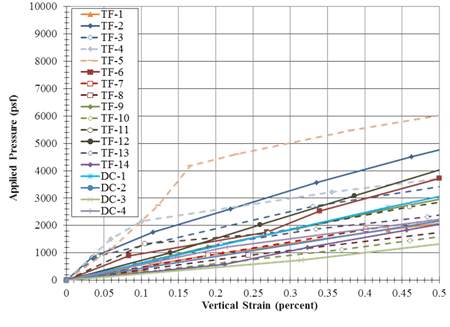
Figure 84. Graph. Load-deformation behavior for the Turner Fairbank PTs at low strain levels.
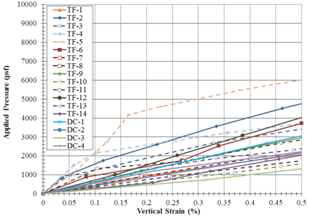
Figure 85. Graph. Normalized load-deformation behavior for the DC and TF PTs up to 0.5-percent vertical strain.
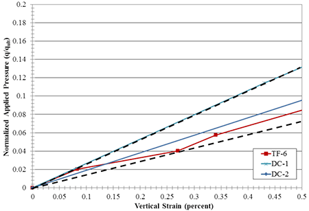
Figure 86. Graph. PTs strictly meeting FHWA GRS abutment design specifications.
In the United States, bridges that receive federal funding for construction must be designed in accordance with the AASHTO LRFD Bridge Design Specifications. AASHTO first adopted a load factor design (LFD) in 1977 for certain portions of the bridge superstructure. In the mid-1990s, the AASHTO Specifications adopted LRFD in geotechnical engineering design based on the work of Barker et al. (1991).(35) Since then, LRFD research has extended to more and more aspects of geotechnical structures.
LRFD in geotechnical design of bridge and building foundations has the following benefits:
A methodology for calibrating the load bearing capacity (strength limit state) of bridge foundations on a GRS abutment is described and presented. Calibration for serviceability limit state is just as, if not more important, since most shallow foundation designs are governed more by serviceability rather than the ultimate limit state; however, the scope of this report is limited to only the strength limit state.(10)
Code calibration is the process of determining values of load and resistance factors. While load factors have already been well established in the AASHTO code, resistance factors for newer types of geotechnical structures must be obtained by calibration. Resistance factors can be calibrated using the following approaches:
Calibration by judgment was the first approach at arriving code parameters, but it suffers from non-uniform margins of safety. Calibration by fitting with ASD essentially results in the LRFD code mimicking the ASD code. It does not necessarily result in more uniform margins of safety or economy. Calibration by fitting was performed for the internal stability design of GRS abutments.(1) The approach adopted herein to calibrate the load bearing capacity of GRS composites is based on reliability theory, which offers a rational process for optimizing the value of resistance factor. The results are then compared with those from calibrating by fitting with ASD.
In general, there are three approaches to estimating resistance factors using reliability analysis: (1) first order second moment (FOSM); (2) advanced first order second moment (AFOSM) and (3) Monte Carlo simulation (MCS). FOSM is the simplest and results in resistance factors that are marginally lower (more conservative) than the AFOSM method, which requires programming of an optimization routine. MCS is only accurate if the load and resistance distributions are correctly modeled. According to Paikowsky (2010), if the statistical parameters are not well-defined, the resulting resistance factor using MCS will not be correct; moreover, if the load and resistance distribution is assumed to be lognormal, MCS will theoretically produce the same results as the FOSM method.(36) Thus, the simpler FOSM approach is adopted in this report.
In the reliability-based approach, the load (Q) and resistance (R) are considered random variables, which can be described by their own probability density functions. One form of margin of safety can be expressed by the difference R - Q where failure occurs when R - Q < 0. In the FOSM approach, R and Q are assumed to have a lognormal distribution; hence a limit state function can be written (figure 87) which is also lognormal. Failure occurs when R/Q is less than 1 or when g(R,Q) is less than 0. The probability density function of figure 87 is shown in figure 88.
The reliability index (ß) is the number of standard deviations between the mean safety margin (ḡ) and failure, where g (R,Q) = 0. According to Paikowsky (2010), many shallow foundations supporting bridge elements have been designed with a target reliability index (ß Τ) between 3.0 and 3.5, which corresponds to a probability of failure of 0.135 percent and 0.023 percent, respectively. (36) Note that these target reliability indices are for foundations on natural soil whereas GRS is an engineered fill.
In LRFD, the factored resistance must be greater than or equal to the factored loads (figure 89).
Where Ф = resistance factor, γi = load factor for load component i, R = resistance and Qi = load component i (e.g., dead load or live load). Many load combinations exist in the AASHTO code; however, resistance factors herein are calibrated using the Strength I load combination only. With only dead and live loads considered, it can be shown that the resistance factor based on FOSM can be calculated according to figure 90.
Where λR , λD, and λL are bias factors for resistance, dead load and live load, respectively, γD and γL are the dead (1.25 for AASHTO assuming Strength I load combination and assuming dead load of structural components and non-structural attachments only; dead load due to the wearing surface is not considered as it usually represents only a small fraction of the total dead weight) and live (1.75 for AASHTO assuming Strength I load combination) load factors, respectively, and VR and VQ are the coefficients of variation (COV) of the resistance and loads, respectively. The bias factor, λ, is the ratio of the measured to the nominal or calculated value; if the variable tends to be over-predicted, then the bias factor will be less than 1. Note that the COV for a variable that is related to several statistically independent variables is merely the square root of the sum of the squares of the various coefficients of variation. For example, figure 91 shows that the COV for factored load (VQ) is equal to the sum of the squares of the COV for dead load (VD) and live load (VL).
It can be seen that in the FOSM method to estimate the resistance factor (figure 90), the random variables are characterized by their first two moments, namely the mean and the standard deviation (which is equal to the product of the coefficient of variation and the mean). Therefore, it is essential to compile the statistics of the load and resistances prior to calibration.
Load Statistics
In the final report to the National Cooperative Highway Research Program (NCHRP) Project No. 20-7/186, Kulicki et al. (2007) provided bias factors and COVs for dead and live loads (table 26). (37) Thus, from (figure 91) and table 26, the COV for factored load is equal to 15.6 percent.
Table 26. Statistics for dead and live loads.
|
Dead Load1 |
Live Load2 |
Bias Factor |
λD= 1.05 |
λ L= 1.14 |
COV |
VD = 10% |
VL = 12% |
1Assumes cast-in-place concrete elements only.
2Assumes HL-93 loading for shear and an average daily truck traffic (ADTT) of 1,000 for two loaded lanes. (10,37)
Resistance Statistics
The variables in the soil-geosynthetic capacity equation (figure 8) and the required reinforcement strength equation (figure 10) include the maximum aggregate size (dmax), the reinforcement strength (Tf) and the passive earth pressure coefficient (Kpr); it is reasonable to assume that the reinforcement spacing (Sv) is not a random variable, therefore the associated fabrication factor is assumed to be unity. Therefore, the COV of the resistance (VR) can be expressed according to figure 92.
Where Vdmax, VTf, VKp and VM are the COVs of dmax, Tf, Kp and the capacity model, respectively.
Note that the ultimate reinforcement strength is usually measured in the laboratory under unconfined conditions; however, it should ideally be measured under confinement to replicate actual in-service conditions. Benjamin et al. (2008) performed numerous measurements of reinforcement strength for woven and non-woven geotextiles in the ground and found the COV for reinforcement strength (VTf) of woven geotextiles was 2.3 and 4.25 percent for the cross-machine and machine directions, respectively. (38) Since woven geotextiles were used in the PTs and are the most commonly used geosynthetic in GRS abutments and IBSs, a VTf value of 4 percent is utilized in this study. For the COV for the passive earth pressure coefficient (VKp), NCHRP Report 651 recommended a value of 15 percent when measuring friction angles with lab tests.(36) The COV for maximum aggregate size (Vdmax) has not yet been investigated, but it is expected to be small; for one reason, the quarries will set their crushers to a given maximum grain size with a high degree of certainty. A value of Vdmax = 5 percent is therefore assumed in this calibration. Additionally, the mean bias factor for the capacity prediction model, using only the data produced in this study, is 0.88 with a COV of about 35 percent (table 23). The resulting COV for resistance (VR) is estimated at 39 percent.
The database of results from this study consists of sixteen cases taken to failure of the GRS composite, four with open-graded backfill (DC-1, DC-2, DC-5, and TF-1) and twelve with well-graded backfill material (TF-2, TF-3, and TF-5 to TF-14). Because the number of cases with open-graded backfill is limited, the present strategy is to arrive at one value for the resistance factor that is applicable to all conditions. With additional testing in the future, separate resistance factors can be calibrated for each soil type, if necessary.
The resistance factor for GRS capacity, calculated according to figure 90, is presented as a function of the ratio of dead load to total load, QD/(QD + QL), and the target reliability index (βΤ ) in figure 93. Note that a QD/(QD + QL) of 0.5 corresponds approximately to a bridge span of about 60 ft, whereas a QD/(QD + QL) of 0.2 corresponds to a bridge span of approximately 250 ft.(39) The bridge span for a GRS-IBS is currently limited to 140 ft (Adams et al. 2011); therefore the resistance factors of interest correspond to QD/(QD + QL) greater than about 0.32. Over this range, the resistance factor varies from 0.26 to 0.28 for βΤ = 3.5, from 0.32 to 0.34 for βΤ = 3.0, and from 0.40 to 0.41 for βΤ = 2.5 using FOSM.
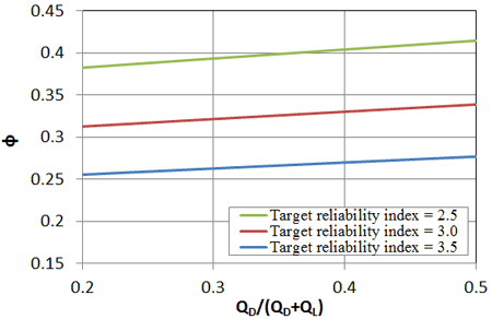
Figure 93. Graph. Resistance factor for footings on GRS composites for different dead to dead plus live load ratios and target reliability indices based on PT series.
Similarly, a reliability analysis was performed using the results of all prior GRS composite testing with a mean bias of 0.95 and a COV for the model of 32 percent (table 24). This slightly increases the resistance factor for the same target reliability indices (figure 94); for the range of QD/(QD + QL) greater than 0.32, the resistance factor varies from 0.31 to 0.33 for βΤ = 3.5, from 0.38 to 0.39 for βΤ = 3.0, and from 0.46-0.48 for βΤ = 2.5 using FOSM.
The resistance factors found through the reliability analysis using the standard reliability indices of 3.0 and 3.5 for bridge foundations are lower than the resistance factor found through calibration by fitting to ASD. For a factor of safety (FS) of 3.5, a resistance factor of 0.45 was estimated for the soil-geosynthetic capacity equation.(1) Through back-calculation, this equates to a reliability index (ß) of about 2.5.
In NCHRP Report 507, Paikowsky et al. (2004) suggested that for redundant foundation systems (such as pile groups), a reliability index of 2.3 was appropriate.(40) With the frequency of the reinforcement spacing, GRS composites can be considered a redundant foundation system as well, with no catastrophic collapse observed at failure for any of the PTs. In addition, Bathurst et al. (2008) suggest that a reliability index of 2.3 is appropriate for the internal stability of reinforced soil walls.(41) This leads to the conclusion that the currently used resistance factor of 0.45, having a reliability index of 2.5, is reasonable for design.
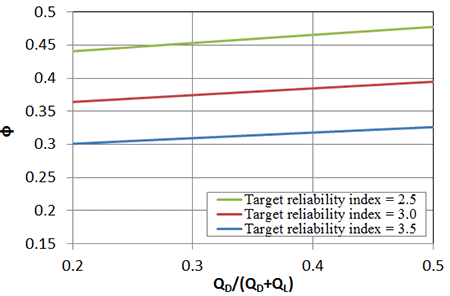
Figure 94. Graph. Resistance factor for footings on GRS composites for different dead to dead plus live load ratios and target reliability indices based on all testing to date.