U.S. Department of Transportation
Federal Highway Administration
1200 New Jersey Avenue, SE
Washington, DC 20590
202-366-4000
Federal Highway Administration Research and Technology
Coordinating, Developing, and Delivering Highway Transportation Innovations
| REPORT |
| This report is an archived publication and may contain dated technical, contact, and link information |
|
| Publication Number: FHWA-HRT-15-033 Date: May 2015 |
Publication Number: FHWA-HRT-15-033 Date: May 2015 |
Data collected from this study are analyzed using a variety of model formulations to develop tools that can be used to estimate critical shear stress and erosion rates for a range of cohesive soils. Field data collected in Illinois and Texas are used to evaluate the recommended model formulations.(8,40) Finally, the model formulations are adapted for use in design.
An overall framework for evaluating the relation between the applied shear stresses and measured erosion rates is required. Two are considered in this study: 1) a power model, and 2) a linear model. Once a model is selected, the critical shear stress and other model parameters may be estimated from the model and laboratory data summarized earlier in table 15. The number of tests for each soil type ranged from 3 to 5, resulting in a total of 72 data points for the 17 soil types.
Initial plotting of the measured shear stress and erosion rate data suggested that a power model of the form given in figure 42 may be appropriate. This model anticipates that no erosion occurs below a certain critical shear stress. Once that critical value is exceeded, the erosion rate will increase with applied shear stress.
![]()
Figure 42. Equation. Power relationship between shear stress and erosion rate
Where:
![]() = Erosion rate, inches/h(mm/h).
= Erosion rate, inches/h(mm/h).
C1 = Multiplier coefficient.
C2 = Exponent.
𝜏 = Applied shear stress, lbf/ft2 (Pa).
𝜏c = Critical shear stress, lbf/ft2 (Pa).
α = Unit conversion constant, 42 for U.S. customary units and 1.0 for S.I.
Regression techniques were applied to develop the parameters 𝜏c, C1, and C2 for each of the 17 soil types. The soil types and estimated shear stress parameters are summarized in table 16. The soil sample ID summarizes the soil type (1 through 6) and the water content. For example, the soil sample indicated with 1W156 is soil mixture 1 with a water content of 15.6 percent. In addition to the critical shear stress and fitted equation constants, the table provides the number of tests with differing applied shear stresses for each soil sample.
Of the 72 tests, several appeared to be unrepresentative of the conditions analyzed or simply outliers. However, that assessment was partially based on pre-analysis hypotheses of how the data should appear. In the initial analyses, as many as seven (10 percent) of the runs were censored and not used in the analyses. Not surprisingly, the decision to exclude data significantly affected the estimated parameters. Without a strong technical basis for excluding the data other than apparent inconsistency with preconceived hypotheses, none of the data were excluded in the final analyses.
Table 16. Estimated critical shear stress parameters for the power model.
Soil Sample |
C1 |
C2 |
𝜏c |
𝜏c (Pa) |
Number of Tests |
R2 |
|---|---|---|---|---|---|---|
1W156 |
0.104 |
2.00 |
0.058 |
2.77 |
5 |
0.992 |
1W165 |
0.104 |
2.00 |
0.065 |
3.12 |
5 |
0.670 |
1W181 |
0.468 |
1.87 |
0.044 |
2.10 |
4 |
0.997 |
2W147 |
0.227 |
1.20 |
0.084 |
4.00 |
5 |
0.995 |
2W167 |
0.062 |
2.00 |
0.052 |
2.47 |
4 |
0.915 |
2W177 |
0.500 |
1.76 |
0.005 |
0.26 |
5 |
0.945 |
3W160 |
0.050 |
1.23 |
0.074 |
3.55 |
4 |
0.427 |
3W180 |
0.064 |
1.65 |
0.021 |
0.99 |
5 |
0.998 |
4W189 |
0.222 |
1.26 |
0.046 |
2.21 |
4 |
1.000 |
4W198 |
0.500 |
1.57 |
0.045 |
2.17 |
3 |
0.983 |
4W217 |
0.500 |
1.86 |
0.041 |
1.97 |
5 |
0.941 |
5W215 |
0.050 |
1.31 |
0.175 |
8.35 |
3 |
0.986 |
5W231 |
0.324 |
1.20 |
0.083 |
3.99 |
4 |
0.872 |
5W248 |
0.442 |
1.45 |
0.073 |
3.51 |
4 |
0.998 |
6W192 |
0.063 |
1.20 |
0.133 |
6.37 |
4 |
0.929 |
6W200 |
0.078 |
2.00 |
0.148 |
7.06 |
3 |
1.000 |
6W231 |
0.486 |
1.20 |
0.078 |
3.72 |
5 |
0.968 |
Although all of the data observations were used, uncritical regression analyses to determine three parameter values-C1, C2, and 𝜏c-could be questionable because each regression analysis included only three to five tests. For this reason, limits were placed on the values for C1 and C2. Values for C1 were constrained to the range of 0.05 to 0.50. As shown in table 16, the minimum value was used for two soil samples (3W160 and 5W215), and the maximum value was used for three soil samples (2W177, 4W198, and 4W217). Similarly, values for C2 were constrained to the range of 1.2 to 2.0. As shown in table 16, the minimum value was used for four soil samples (2W147, 5W231, 6W192, 6W231), and the maximum value was used for four soil samples (1W156, 1W165, 2W167, and 6W200).
No limit was placed on the value of 𝜏c. The resulting unconstrained critical shear stress estimates ranged from 0.005 lbf/ft2 (0.26 Pa) for soil sample 2W177 to 0.175 lbf/ft2 (8.35 Pa) for soil sample 5W215. The median critical shear stress for the 17 soil samples was 0.065 lbf/ft2 (3.12 Pa).
Fourteen of the R2 values for the regressions exceeded 0.90, with seven exceeding 0.99. The three with lower R2 values (1W165, 3W160, and 5W231) included most of the data points that had been previously considered for exclusion but were retained in the analyses.
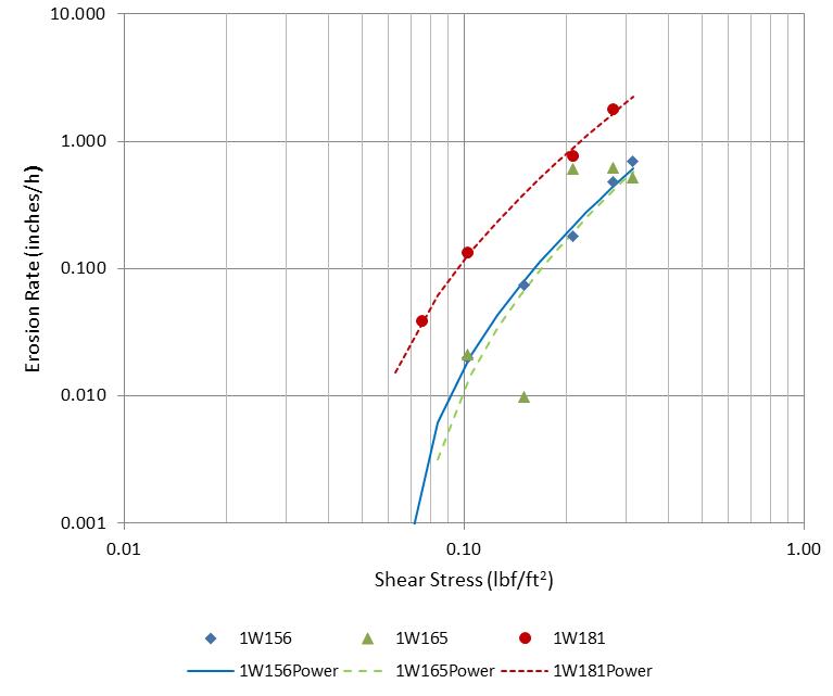
Figure 43 illustrates the observed and fitted data for the three soil types of soil index 1. Soil 1W165 includes several observations that do not exhibit a monotonically increasing erosion rate with shear stress. For this reason, some of these data were considered for censoring. However, placing limits on the regression parameters provided reasonable estimated parameters for this soil type as well as the other two more consistent data sets for this soil index.
1 inch = 25.4 mm.
1 lbf/ft2 = 47.8 Pa.
Figure 43. Graph. Measured and fitted power model for soil index 1
The linear model shown in figure 44 was also evaluated with the laboratory data. Unlike the power law model, the critical shear stress is not explicit in the equation. However, it can be estimated by solving for the applied shear stress when the erosion rate is zero.
![]()
Figure 44. Equation. Linear relationship between shear stress and erosion rate
Where:
![]() = Erosion rate, inches/h (mm/h).
= Erosion rate, inches/h (mm/h).
C3 = Multiplier coefficient, dimensionless.
C4 = Constant, inches/h (mm/h).
𝜏 = Applied shear stress, lbf/ft2 (Pa).
α = Unit conversion constant, 1.88 for U.S. customary units and 1.0 for S.I.
Regression techniques were used to develop the parameters for the linear model that are summarized in table 17.
Table 17. Estimated critical shear stress parameters for the linear model.
Soil Sample |
C3 |
C4 (mm/h) |
C4(in/h) |
𝜏c (Pa) |
𝜏c (lbf/ft2) |
Number of Tests |
R2 |
|---|---|---|---|---|---|---|---|
1W156 |
1.03 |
5.88 |
0.232 |
5.74 |
0.120 |
5 |
0.929 |
1W165 |
1.33 |
6.92 |
0.272 |
5.20 |
0.109 |
5 |
0.818 |
1W181 |
2.61 |
10.46 |
0.412 |
4.01 |
0.084 |
5 |
0.933 |
2W147 |
0.23 |
1.07 |
0.042 |
4.64 |
0.097 |
5 |
0.969 |
2W167 |
0.69 |
3.90 |
0.154 |
5.65 |
0.118 |
5 |
0.783 |
2W177 |
2.14 |
4.74 |
0.187 |
2.21 |
0.046 |
5 |
0.977 |
3W160 |
0.04 |
0.24 |
0.010 |
5.50 |
0.115 |
5 |
0.734 |
3W180 |
0.27 |
1.09 |
0.043 |
4.05 |
0.085 |
5 |
0.977 |
4W189 |
0.27 |
0.93 |
0.037 |
3.41 |
0.071 |
5 |
0.997 |
4W198 |
1.23 |
4.33 |
0.170 |
3.51 |
0.073 |
5 |
0.990 |
4W217 |
2.74 |
10.17 |
0.400 |
3.72 |
0.078 |
5 |
0.976 |
5W215 |
0.06 |
0.60 |
0.024 |
9.33 |
0.195 |
5 |
0.952 |
5W231 |
0.39 |
2.07 |
0.081 |
5.27 |
0.110 |
5 |
0.988 |
5W248 |
0.85 |
4.25 |
0.167 |
4.99 |
0.104 |
5 |
0.977 |
6W192 |
0.05 |
0.29 |
0.012 |
6.00 |
0.125 |
5 |
0.836 |
6W200 |
0.49 |
4.59 |
0.181 |
9.36 |
0.196 |
5 |
0.978 |
6W231 |
0.45 |
1.86 |
0.073 |
4.17 |
0.087 |
5 |
0.940 |
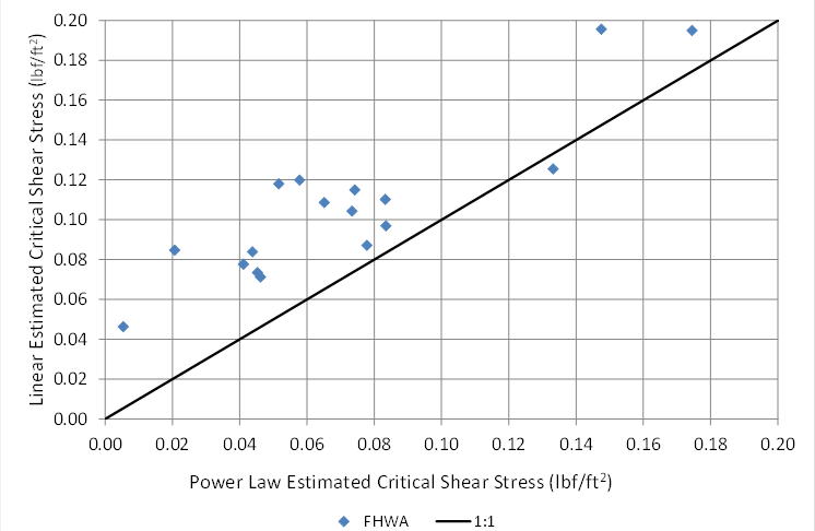
Critical shear stress is a parameter common to both models. A comparison between the estimated values using the linear model and power model is shown in figure 45. With one exception, the linear model results in a higher estimate of critical shear stress compared with the power model. Although the two estimates correlate to a certain degree, the differences highlight the challenge in estimating critical shear. As shown here, the type of model used will have an influence on the outcome. This uncertainty is further amplified because the measurements may also differ based on the test apparatus that is used.
The power law model is selected primarily for two reasons. First, the erosion rates measured in the ESTD do not appear to be linear versus applied shear stress, which explains the generally better fits with the power law model. Second, the power law estimates are generally smaller and, therefore, more conservative than the estimates from the linear model.
1 lbf/ft2 = 47.8 Pa.
Figure 45. Graph. Estimated critical shear stress comparison
One of the objectives of this study is to develop a method to estimate critical shear stress from more readily accessible soil characteristics so that testing using the ESTD for every soil is not required. The following soil parameters were evaluated for their utility for predicting critical shear stress for a cohesive soil:
Three model types were considered for predicting critical shear stress. Two are from the literature, and the third is a power law formulation.
In addition to the data collected for the current study (FHWA data), two other data sets are used. The Illinois Department of Transportation investigated 22 field samples for their erosion characteristics.(8) Another 13 field samples from Texas were collected and analyzed by researchers.(40) Figure 46 displays a plot of the FHWA, Illinois, and Texas data with respect to the parameters used in the USCS: LL and PI. The "A-Line" shown in the figure divides the clay from the silt soils. Above the A-line represents those soils classified as clays. All but one of the Illinois data points falls in this classification. Those soils above the A-line that have a PI between 0.04 and 0.07 are classified as a clay/silt mix (CL-ML).
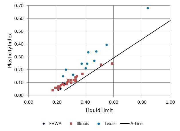
Figure 46. Graph. Comparison of FHWA, Illinois, and Texas soil data
The FHWA data are located within the Illinois data but within a much more limited range of LL and PL, specifically for a PI of less than 0.1 and an LL of less than 0.3. The Texas data also show a broad range of values, although they tend to exhibit somewhat higher plasticity indices for a given LL. Because all three data sets are used in the analyses that follow, the differences in their characteristics may become important in the evaluation.
Selected soil sample characteristics are summarized in table 18 including the number of observations in each data set. The FHWA data set is bounded by a narrower range of values than are the Illinois or Texas data in part because the latter two data sets are field collected. The Texas data generally displays the widest range of characteristics even though it is a smaller data set. It includes observations with higher water content, lower saturation, higher PI, higher void ratio, and a wider range of median grain size than the other two data sets. Neither the Illinois nor Texas data sets include specific information on the types of clay present in the soils.
Table 18. Data set parameter summary.
Parameter |
Statistic |
FHWA |
Illinois |
Texas |
|---|---|---|---|---|
Number of Data Points |
n |
17 |
22 |
13 |
Critical Shear Stress (lbf/ft2) |
Minimum |
0.0054 |
0.0207 |
0.0038 |
Median |
0.0652 |
0.1808 |
0.0163 |
|
Maximum |
0.1745 |
0.4093 |
0.0878 |
|
Fraction of Fines |
Minimum |
0.51 |
0.46 |
0.30 |
Median |
0.70 |
0.73 |
0.87 |
|
Maximum |
0.80 |
0.96 |
0.99 |
|
Water Content |
Minimum |
0.147 |
0.098 |
0.173 |
Median |
0.189 |
0.222 |
0.221 |
|
Maximum |
0.248 |
0.450 |
0.401 |
|
Adjusted Water Content |
Minimum |
0.258 |
0.104 |
0.202 |
Median |
0.290 |
0.303 |
0.281 |
|
Maximum |
0.355 |
0.597 |
0.576 |
|
Saturation |
Minimum |
0.928 |
na |
0.751 |
Median |
0.975 |
na |
0.916 |
|
Maximum |
1.098 |
na |
1.291 |
|
Plasticity Index |
Minimum |
0.043 |
0.040 |
0.151 |
Median |
0.070 |
0.105 |
0.270 |
|
Maximum |
0.097 |
0.250 |
0.939 |
|
Unconfined Compressive Strength (lbf/ft2) |
Minimum |
980 |
360 |
420 |
Median |
1,630 |
1,250 |
1,230 |
|
Maximum |
3,970 |
15,070 |
5,020 |
|
Void Ratio |
Minimum |
0.43 |
na |
0.46 |
Median |
0.52 |
na |
0.63 |
|
Maximum |
0.66 |
na |
0.93 |
|
Median Grain Size (inches) |
Minimum |
0.00063 |
0.00016 |
0.00005 |
Median |
0.00083 |
0.00074 |
0.00187 |
|
Maximum |
0.00256 |
0.00510 |
0.01043 |
The USDA developed equations for estimating permissible shear stress for fine grained cohesive soils for the purposes of evaluating channel lining stability.(41) Permissible shear is that level of stress below which the soil will resist and not erode. Different terms (permissible and critical shear stress) can be considered to be describing the same soil behavior. The basic formula is given in the equation in figure 47.
![]()
Figure 47. Equation. USDA equation for permissible shear stress
Where:
𝜏p = Soil permissible shear stress, lbf/ft2 (Pa)
PI = Plasticity index, dimensionless.
e = Void ratio, dimensionless.
c1, c2, c3, c4, c5, c6 = Coefficients.
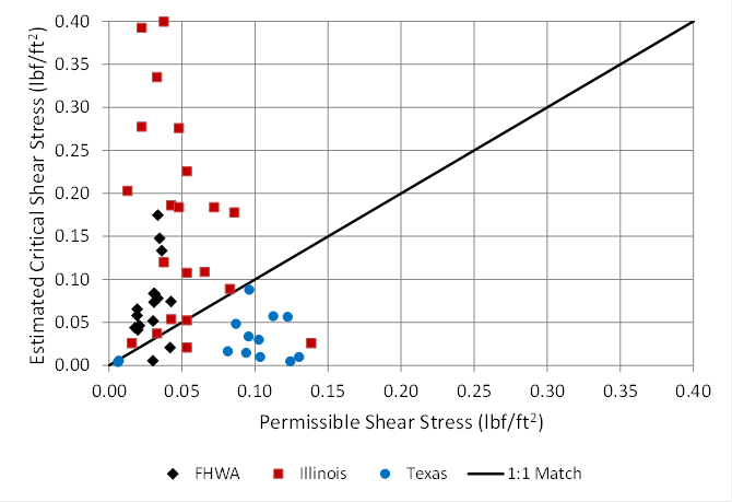
The coefficients are selected based on the USCS type of the soil. Figure 48 shows that the permissible shear stress computed from the USDA equation does not correlate well with critical shear stresses estimated from the data developed in this study. With few exceptions, the estimated critical shear stress is higher for the FHWA data.
The figure also includes data collected from both Illinois and Texas. (A void ratio of 0.5 was assumed for the Illinois data.) The estimated critical shear stresses for the Illinois data are also generally higher than the USDA permissible shear stresses. For many data points, they are much higher. For the Texas data, the reverse is true: the estimated critical shear stresses are generally less than the permissible shear stresses computed from the USDA equation. These results suggest that the USDA model is not appropriate for estimating critical shear stress for these data sets.
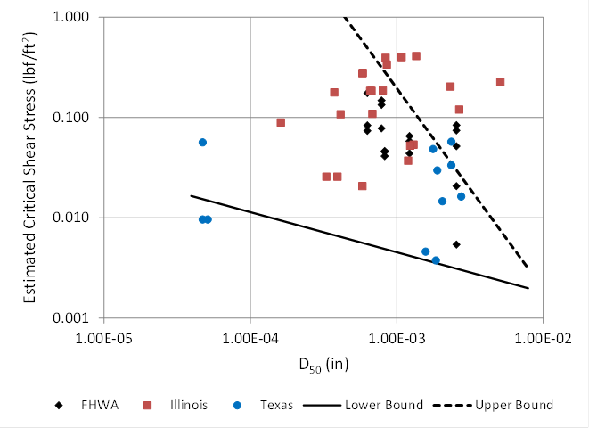
HEC-18 provides two equations for defining high and low bounds on critical shear stress for fine-grained soils attributed to Briaud.(42) Both equations use the median grain size, D50, as the independent variable. Although commonly used as a predictive parameter for noncohesive soils where shear stress resistance increases with grain size, the use of D50 for cohesive soils is less frequent. As given in figure 49 and figure 50, these equations indicate increasing critical shear stress with a decrease in grain size. This decrease may be an indication of an increase in electrochemical forces with smaller particle size. Both equations are applicable only to soils with D50 less 0.0079 inches (0.2 mm).
1 lbf/ft2 = 47.8 Pa.
Figure 48. Graph. Comparison of permissible and critical shear stress
![]()
Figure 49. Equation. Briaud equation for critical shear stress lower bound
Where:
α = Unit conversion constant, 2.85x10⁻⁴ for U.S. customary units and 0.05 for S.I.
![]()
Figure 50. Equation. Briaud equation for critical shear stress upper bound
Where:
α = Unit conversion constant, 1.9x10⁻⁷ for U.S. customary units and 0.006 for S.I.
A comparison of the estimated shear stresses from this study with the lower and upper bounds is provided in figure 51, which also includes comparisons for the Illinois and Texas data. A small number of data observations exhibit critical shear stresses less than the lower bound equation, while several data points have critical shear stresses that exceed the upper bound equation. These observations suggest that these equations are limited in their value for providing bounds for critical shear stress in many cohesive soils.
1 inch = 25.4 mm.
1 lbf/ft2 = 47.8 Pa.
Figure 51. Graph. Comparison of critical shear stress with Briaud bounds
Power models are applied in a variety of technical areas and are a common way of describing a relation between a dependent variable and one or more independent variables. The general form is shown in figure 52.
![]()
Figure 52. Equation. General power model
Where:
y = Dependent variable.
xi = Independent variables.
a = Coefficient.
bi = Exponents.
After a series of analyses that considered degree of correlation, statistical significance, and physical meaning, a relationship was developed from the FHWA data to predict critical shear stress for a soil. The parameters with the strongest correlations to critical shear stress in the FHWA data were the water content, w; fraction of fines, F; plasticity index, PI; and unconfined compressive strength, qu.
HEC-18 notes that "cohesive soils do not have intrinsic strength properties."(2) It further states that the presence of fine grains (less than 0.003 inches (0.075 mm)) in a soil will alter the properties from that which would be indicated from grain size alone. Soils with at least 10 percent fines will exhibit some cohesion, and soils with as much as 35 percent fines will be dominated by cohesion. Therefore, the use of fines in the predictive equation is logical.
The water content provides a proxy for the degree of consolidation of the soil, which reflects the physical arrangement of the grains. Assuming the soil is close to 100-percent saturation, the higher the water content, the less packed the grains are likely to be, thereby reducing the resistance to initiation of erosion. It was observed in several of the regression analyses that water content and the percentage fines yielded exponents of approximately the same magnitude but opposite signs. This observation led to the decision to combine them as an "alternative" water content, w/F, which represented the mass of water relative to the mass of the fines rather than the entire soil mass.
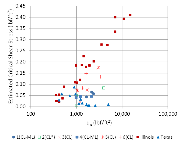
With respect to unconfined compressive strength, some researchers using field data from Illinois found a strong relationship between critical shear strength and unconfined compressive strength.(8) The data from the current study shows some correlation between the two but weaker than that found in the Illinois data. Figure 53 summaries the current data and the Illinois and Texas data. The Illinois data are shifted to the left from the FHWA data, demonstrating that the same predictive relationship cannot be used for both data sets without accounting for this shift. For a given value of qu, the Illinois data suggest higher critical shear stresses. The Texas data do not show an increasing relation of critical shear stress with unconfined compressive strength.
There are several possible explanations for this shift between the current data and those from Illinois. One is that critical shear stress was estimated differently in the two studies. Because this property is not directly measured, there may be methodological differences between the two studies. Second, the predominant type of clay in the soils may have different electrochemical properties that cause the shift. Finally, the shift may result from the influence of other soil characteristics on critical shear stress.
Initial regression analyses with w/F, PI, and qu showed that the variable qu was statistically marginal in explaining the variation in critical shear stress when used in conjunction with the other two variables. Therefore, qu was dropped from some evaluations and included in others to compare.
Regression analyses using only w/F and PI yielded an exponent of -7.2 for w/F and 1.5 for PI. An exponent with the magnitude of 7.2 is very high and indicates extreme sensitivity to adjusted water content variable. The range of adjusted water content in the FHWA data is from 0.258 to 0.355. This range is narrow compared with both the Illinois (0.104 to 0.597) and Texas (0.202 to 0.576) data sets. Therefore, it was decided to limit the magnitude of this exponent to 2.0 to achieve a potentially more robust model. The recommended power model is shown in figure 54.
1 lbf/ft2 = 47.8 Pa.
Figure 53. Graph. Critical shear versus unconfined compressive strength

Figure 54. Equation. Predictive relation for critical shear stress
Where:
𝜏c = Critical shear stress, lbf/ft2 (Pa).
w = Water content, dimensionless ratio.
F = Fraction of fines by mass (< 75µm), dimensionless ratio.
PI = Plasticity index, dimensionless ratio.
qu = Unconfined compressive strength, lbf/ft2 (Pa).
α = Unit conversion constant, 0.01 in U.S. customary units and 0.1 in S.I.
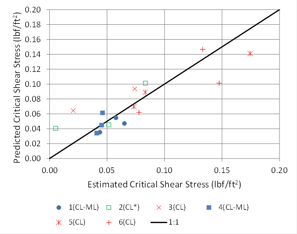
The R2 of the equation is 0.73 and was only reduced marginally by constraining the exponent on adjusted water content. With this equation, 7 of the 17 predicted critical shear stresses were higher than the estimated critical shear stresses. A comparison of the critical shear stress predicted by the equation in figure 54 with those estimated and reported in table 16 is provided in figure 55. The reference value is intentionally called "estimated" because it is not a directly measurable or observed property but must be calculated as described previously.
The key in the figure provides the soil index number with an indicator of the soil classification CL or CL-ML. Soil index 2 is indicated as CL* because the PI for this soil is 7.0 percent, which is the dividing value between CL and CL-ML soils. With the exception of three soil samples, the predicted and estimated critical shear stresses are less than or equal to 0.10 lbf/ft2 (5 Pa).
1 lbf/ft2 = 47.8 Pa.
Figure 55. Graph. Comparison of predicted versus estimated critical shear stress
Using the relation in figure 54, a critical shear stress for cohesive soils may be computed based on the water content, w; the fraction of fines, F; the plasticity index, PI;and the unconfined compressive strength, qu. In some situations, it may be difficult to reliably estimate the water content of a soil sample, or it may be desirable to assume that the sample will be saturated during an erosion event. In either of these cases, the water content, w, may then be estimated from the soil void ratio and specific gravity assuming that the soil is 100-percent saturated. This relation is provided in figure 56.

Figure 56. Equation. Water content at 100-percent saturation
Where:
w = Water content, dimensionless ratio.
e = Void ratio, dimensionless ratio.
Sg = Specific gravity of the soil, dimensionless ratio.
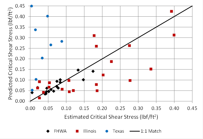
The predictive equation for critical shear stress in figure 54 may also be applied to the Illinois and Texas data. The results are shown in figure 57. Of the 22 Illinois data points that were in the range of property values required for the predictive equation, critical shear stress is overpredicted for 5 of the observations. Of the 13 Texas data points, critical shear stress is overpredicted for all of the observations, with 5 of the data points not shown on the plot because the predicted critical shear stress exceed 0.45 lbf/ft2 (21 Pa).
1 lbf/ft2 = 47.8 Pa.
Figure 57. Graph. Critical shear stress comparison with FHWA, Illinois, and Texas data
Further examination of the Illinois and Texas data reveals that these field data sets exhibit wider ranges of soil characteristics for key parameters than found in the FHWA laboratory data on which the predictive equation is based. For example, the maximum PI value for the FHWA data is 0.097, while it is 0.250 and 0.939 for the Illinois and Texas data, respectively. Similarly, the maximum value of the fraction of fines, F, in the FHWA data set is 0.80, while this value goes up to 0.96 and 0.99 for the Illinois and Texas data.
When data with a PI of greater than 0.25 or a fraction of fines greater than 0.9 are discarded, the performance of the equation predicting critical shear stress for both the Illinois and Texas data improves significantly. For the Illinois data set, four data points are discarded, all for having a fraction of fines greater than 0.9. The resulting R2 value is 0.52. For the Texas data set, 8 of the 13 data points are discarded, all but one of which has a PI greater than 0.25. The R2 value is still very poor (less than zero), but deleting the out-of-range data retained the observations with the best fit.
An additional data attribute that was not available for this study is the characterization of the types of clay predominant in the Illinois and Texas data. The clay composition will likely affect the erosion properties of cohesive soils because the electrochemical behavior relates to the soil behavior but differs with the type of clay. More investigation on this point is warranted.
Two other potentially important differences between the FHWA data and either the Illinois or Texas data are as follows: 1) the FHWA samples were prepared in a controlled laboratory environment, while the Illinois and Texas data were field samples, and 2) the FHWA estimates of critical shear stress were derived from tests using the ESTD, while the Illinois and Texas critical shear stress values were derived by testing with the EFA. Further investigation into the significance of these two factors is also warranted.
Numerous alternative formulations of the power law were evaluated regarding both which and how many soil parameters to include. None were found that were effective in predicting the estimated critical shear stresses.
Neither the USDA nor the Briaud bounding equations performed well in explaining the current data or the Illinois or Texas data. The proposed power law formulation developed using the current data performed reasonably well when validating it against the Illinois data once data outside the applicable range were removed. The equation was also applied to the Texas data, but these data seem to be predominately outside the range of characteristics under which the equation is valid, particularly PI and fraction of fines.
To use the equation in figure 42, the coefficient, C1, and exponent, C2, must also be computed. The soil parameters previously considered for development of a predictive equation for critical shear were also considered for predicting C1 and C2. After several analyses, the equation in figure 58 was selected for the coefficient C1.
![]()
Figure 58. Equation. Predictive relation for C1
Where:
C1 = Multiplier coefficient for the erosion model.
qu = Unconfined compressive strength, lbf/ft2 (Pa).
PI = Plasticity index, dimensionless ratio.
α = Unit conversion constant, 14.2 in U.S. customary units and 680 in S.I.
The R2 for this equation is 0.35. Although not a statistically strong relation, the parameters included reflect that as compressive strength and PI increase, C1 and, therefore, the erosion rate decrease. The predicted and estimated values are compared in figure 59. A weakness in this relation is that for estimated (observed) values of C1 greater than 0.2, the equation underpredicts, while for values less than 0.2, the equation overpredicts.
The exponent C2 was estimated to range from 1.2 to 2.0 as was summarized in table 16. Higher values of this exponent correspond to higher erosion rates. The soil parameters listed previously were examined for their utility in predicting this exponent. However, a satisfactory relationship was not found. Therefore, a constant value of C2 that provides the best fit to the erosion data was determined to be 1.8.
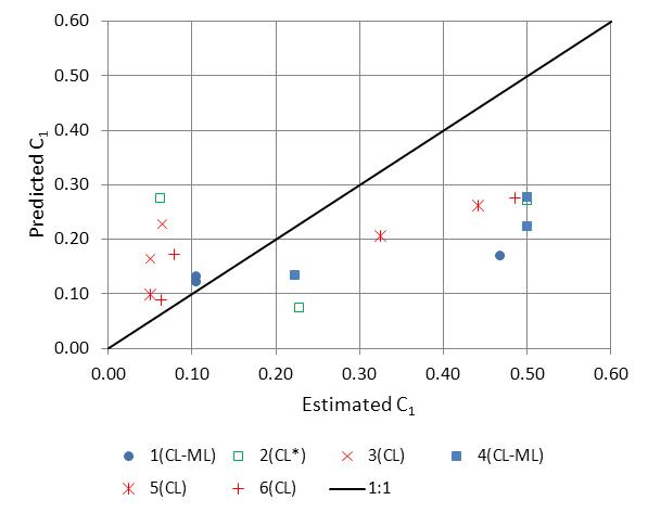
Figure 59. Graph. Predictive relation for the multiplier coefficient
The resulting best-fit model is summarized in figure 60, where critical shear stress, 𝜏c, is calculated from the equation in figure 54 and C1 is calculated from the equation in figure 58.
![]()
Figure 60. Equation. Erosion rate model
Where:
α = Unit conversion constant, 42 in U.S. customary units and 1.0 in S.I.
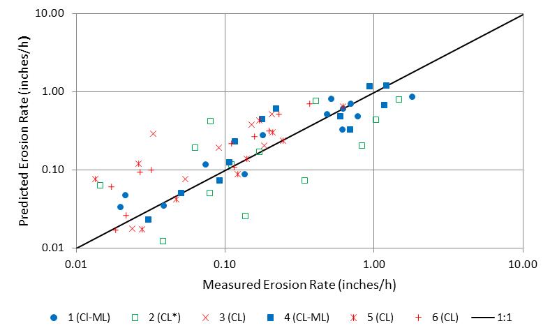
These equations are applied to the 72 erosion test data sets from the current study. The R2 for predicting the erosion rate is 0.61, with 60 percent of the calculated erosion rates overpredicting the measured rates. Overprediction in this context would be conservative. A plot of the predicted and measured erosion rates is provided in figure 61.
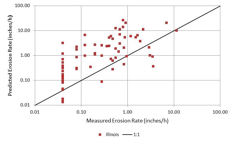
The equation for estimating erosion rate was also applied to the Illinois data. The results are summarized in figure 62. Excluding the soil samples with a PI greater than 0.25 and fraction of fines greater than 0.9, 74 of the 91 data observations were overpredictions (conservative). Several of the measured erosion rates appear on a vertical line at 0.0394 inches/h (1.0 mm/h). This value was the lowest reported nonzero value in the data set.
The Texas data set did not include erosion rate/shear stress pairs. Therefore, these data could not be used to validate the proposed erosion model.
1 inch = 25.4 mm.
Figure 61. Graph. Predicted versus measured erosion rates
1 inch = 25.4 mm.
Figure 62. Graph. Predicted versus measured erosion rates with Illinois data
For design purposes, conservative equations that reduce the risk of underpredicting erosion are desired. The previous equations represent relations that offer the best fit to the FHWA laboratory data. These equations may be adjusted by changing the coefficient C1 in the equation in figure 60 and the initial coefficient in the equation in figure 54.
An underprediction rate of no more than 10 percent was selected as the goal for an appropriate design equation, given the relatively small number of measured data points and the high variability of the observations. Given this goal, the design equation for critical shear stress is seen in figure 63. The only change is a reduction in the initial coefficient by 30 percent, thereby reducing the estimates of critical shear stress by 30 percent when applied to design situations.

Figure 63. Equation. Design equation for critical shear stress
Where:
αd = Unit conversion constant for design, 0.007 in U.S. customary units and 0.07 in S.I.
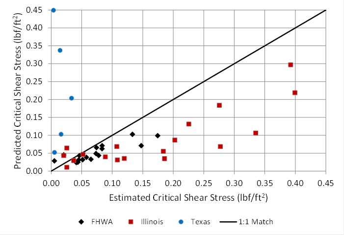
Figure 64 illustrates a comparison of the predicted critical shear stress for design with the estimated critical shear stress values. In this case, underpredicting is considered to be conservative. The figure shows that, with the exception of the Texas data, the predictive equation underpredicts critical shear stress as is desired. Illinois and Texas data not within the recommended ranges for PI and fraction of fines are excluded from the analysis.
For the FHWA data, the ratio of the predicted critical shear stress to the estimated critical shear stress ranges from 0.48 to 5.2 with a median value of 0.66. Similarly, for the Illinois data, the ratio ranges from 0.19 to 2.5 with a median value of 0.50. The median values provide a measure of the conservative nature of the critical shear stress equation. As seen in figure 64, those data points that do not represent conservative estimates with a ratio of greater than 1 (above the 1:1 match line) occur at the lower end of the range of critical shear stresses.
The design equation for C1 is given in figure 65. The only change is an increase in the initial coefficient by 61 percent when applied for design so that no more than 10 percent of the estimates are underpredictions.
Figure 66 illustrates a comparison of the predicted critical erosion rates for design with the measured erosion rates. In this case, overpredicting is considered to be conservative. The figure shows that the predictive equation overpredicts erosion rates as desired.
For the FHWA data, the ratio of the predicted erosion rates to the measured erosion rates ranges from 0.5 to 75 with a median value of 2.8. Similarly, for the Illinois data, the ratio ranges from 0.1 to 83 with a median value of 3.1. The median values provide a measure of the conservative nature of the erosion rate model. As can be seen from figure 66, those data points that do not represent conservative estimates with a ratio of less than 1 (below the 1:1 match line) occur at both the lower and upper end of the range of erosion rates.
1 lbf/ft2 = 47.8 Pa.
Figure 64. Graph. Design equation for critical shear stress compared with data
![]()
Figure 65. Equation. Design equation for C1
Where:
αd = Unit conversion constant for design, 23 in U.S. customary units and 1100 in S.I.
Because the FHWA data included erosion tests up to 0.31 lbf/ft2 (15 Pa) and the Illinois validation data included tests up to 1.67 lbf/ft2 (80 Pa), it is recommended that the equation in figure 60 be applied only for situations in which the bed shear stress is less than or equal to 2.1 lbf/ft2 (100 Pa). Additional research on the response of these soils to higher shear stresses is needed.
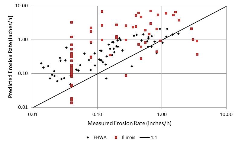
1 inch = 25.4 mm.
Figure 66. Graph. Design equation for erosion rate compared with data