
This appendix is a self-contained write-up concerning the FHWA TNM vehicle emission levels analysis and the adequacy of measured data sets. Challenges Computing Reference Energy Mean Emission Level Coefficients using Small Datasets
Introduction
The Federal Highway Administration's Traffic Noise Model (FHWA's TNM), which is used "as a means of aiding compliance with policies and procedures under FHWA regulations"1, uses Reference Energy Mean Emission Levels (REMELs)2 as the foundation of its source sound level computations. TNM has REMEL data for two vehicle operating conditions: cruise and full-throttle; five standard vehicle types: automobiles, medium trucks, heavy trucks, buses, and motorcycles; and for five pavement types, dense-graded asphalt concrete (DGAC), open-graded asphalt concrete (OGAC), Portland cement concrete (PCC), and Average (a combination of DGAC and PCC). TNM also has the ability to accept limited REMEL data for user-defined vehicle types. Various agencies are also interested in developing custom REMELs for new pavements. Although TNM version 2.5 does not support user defined REMELs for new pavements, this functionality may be implemented in the future.
The intent of this document is to 1) provide an overview of the process for computing REMEL coefficients, 2) to identify conditions where the REMEL model is and is not applicable, and 3) to provide guidance on issues related to developing REMELs when using small datasets. The process for computing both overall A-weighted level coefficients, A to C, and for computing the spectral coefficients, D1 to K2, will be reviewed and a procedural flowchart will be developed to help guide the acoustician through the process of selecting the correct steps for their dataset. This overview will include a discussion of both historical recommendations and recommendations based on current statistical processing capabilities. Following this overview, several problem data sets will be considered and recommendations to deal with these datasets will be made. These recommendations will include the collection of additional data, the use of related existing data to supplement the modeling, and alternate methods to aggregate the data. In some cases the REMEL model will not be suitable. In such cases explanation as to why a dataset is not suitable for REMEL modeling will be given.
Overview of REMEL Model
The REMEL model was developed for use with the FHWA's Traffic Noise Model from individual vehicle pass-by data measured at (or corrected to) 50 feet from the center of the traffic lane of interest, 5 feet above the plane of the road surface. Key input parameters include: pavement type, operating condition, vehicle type, vehicle speed, maximum A-weighted sound pressure level during the pass-by event, vehicle speed at pass-by, the one-third octave band level associated with the maximum A-weighted sound pressure level, and the event quality, that is, whether or not there was contamination from other sound sources during the measurement.
The model assumes that the sound pressure level is an energy sum of two levels, a constant component, which can be determined from the idle level, and a speed dependent component, which can be determined from the level over a sufficient speed range. The combination of the two components is illustrated in Figure 1. In this example the overall level is dominated by the constant component below speeds of about 10 mph. Between 10 and 20 mph, there is a transition where both components significantly affect the overall level. Above 20 mph, the speed dependent component dominates.
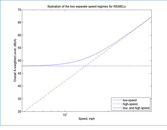
Figure 1: Overall A-weighted Level According to REMEL Model
The overall A-weighted sound pressure level model is given by:
Equation 1: REMELs Model for Overall A-weighted Level

Here, LA,max is the energy mean overall A-weighted level associated with the maximum level during pass-by, s is the speed in miles per hour; A, B, and C are REMEL coefficients associated with a specific vehicle type, pavement type, and engine operating condition; and DEc and DEb are corrections to convert from a level mean to an energy mean. C + DEc account for the constant component. A accounts for the slope of the speed dependent component. B + DEb account for the offset of the speed dependent component, that is, an increase in B + DEb will result in the sloped portion of the overall level being shifted upwards in Figure 1. Note that there is no DEA because the correction from level mean to energy mean for the speed dependent component is handled in the B coefficient. It is also important to note that DE is given not by the equation in Section 6.1.2 of Reference 2, but by:
Equation 2: Adjustment from Level Mean to Energy Mean
where, N is the number of samples, ri = Li - L. Li is the overall A-weighted level for the ith sample, and L is the linear average over all samples. The derivation for Equation 2 is given in Reference 31.
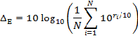
In addition to the overall A-weighted sound pressure level, the REMEL model accounts for the emission spectral shape. REMELs model the relationship between spectral content using the polynomial relationship given in Equation 3
Equation 3: REMEL Model for One-Third Octave Band Spectra (Level Mean)
where, LA,max is the level mean overall A-weighted level associated with the maximum level during pass-by, s is the speed in miles per hour, f is the nominal center frequency of the one-third octave bands, and A1 through J2 are coefficients determined during the curve fitting process. An example of the spectral shapes obtained from this process is given in Figure 2.
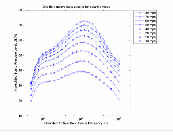
Figure 2: A-weighted Spectral Shape According to REMEL Model
Note, this model, does not include an adjustment from the level mean to the energy mean, therefore, this model represents the level mean. The overall energy mean and spectral level mean models can be unified by subtracting the overall A-weighted level mean as a function of speed alone from Equation 3 and then adding Equation 1.
Equation 4: : REMEL Model for One-Third Octave Band Spectra (Energy Mean)
where, LA,max is the energy mean overall A-weighted level associated with the maximum level during pass-by and K1 and K2 remove the overall A-weighted level mean as a function of speed associated with Equation 3. Note, that since the first part of Equation 4 accounts for the adjustment from level mean to energy mean, and the second part of the equation provides no net change to the overall A-weighted level, an adjustment from level mean to energy mean is not required for the second part of Equation 4.
Guidance on Computing REMELs (and discussion of Sensitivities)
Although the REMEL model is straightforward, formal guidance is useful to help avoid pitfalls to modeling vehicle noise emissions using the approach. In this section, general principles for assuring data distribution in an ideal case will be discussed. Figure 3 shows the speed distribution for the auto baseline REMELs used for TNM 2.5. This distribution illustrates several key features of a good speed distribution:
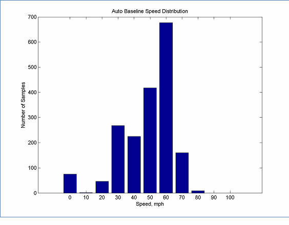
Figure 3: Data Distribution for Auto Baseline REMELs used in TNM 2.5
It is clear that having both high speed and low speed data allows for accurate estimates of both the A and B as well as the C coefficients is required. Assuming that the estimation of C is not dependent on A or B, Equation 1 can be reformulated as two linear equations, solving for C separately from A and B.
This allows commonly available analysis tools to be used to solve for these parameters rather than having to rely on specialized non-linear solvers. However, in order to solve for the parameters separately, only data for the appropriate speed range should be used. When solving for C, only speeds where the low speed level dominates should be used. When solving for A and B, only speeds where the high speed level dominates should be used. The relationship between the data distribution and the linear portions of the curve can be seen in Figure 4. Having a speed distribution as shown in Figure 3 and Figure 4 allows all data to be used without risk of biasing the curve fitting results.
The independence assumption is valid provided that there is no relationship between the level at idle and at high speeds. A counter example to this independence assumption would be if all vehicles with higher than normal idle levels had higher than normal levels at, say, 55 mph. This would most likely happen if the vehicle's engine was the dominant source at high speed, but even then this is not a guarantee of dependency, it would still be possible for the engine operation to be sufficiently different at idle and at cruise that no relationship between the levels could be found. If there is doubt about the independence assumption, then it should be tested5. In cases where there is a significant dependence, then the non-linear form, Equation 1, must be used.
For the high speed portion of the curve, a slope needs to be estimated. This can only be done with confidence if the speed range creates a mean change in level greater than the random variation about the mean. If the data range is too small then the greatest portion of the variance will be explained by random factors rather than the growth of level associated with speed. Finally, a practical consideration is that REMELs are developed with a specific application in mind. Typically, this is to develop emissions for modeling traffic related noise adjacent to highways. In such cases, it is most useful to have the highest degrees of confidence in the speed range associated with highway traffic. In general it can be stated that, the greater the number of samples, the greater the confidence of a parameter's estimated value.
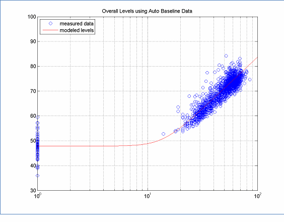
The data in this figure is located here, for measured data and here, for modeled levels.
Figure 4: Ideal Speed Distribution of Data for Overall Levels with Respect to Curve Shape
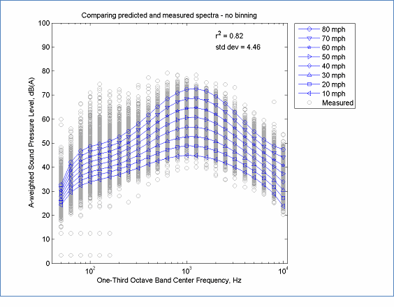
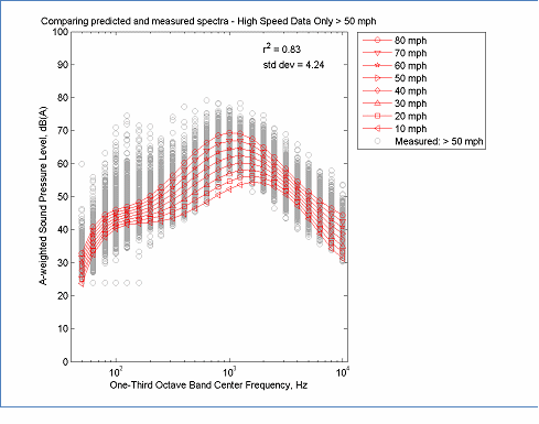
Using an appropriate speed distribution for the data also results in spectral profiles that are well behaved as a function of speed, that is, the curves are anchored at the speed extremes to the data and the intermediate speed curves fit the data well. This can be seen in Figure 5, where the spectral curves fit the data very well and have smooth transitions from low speed to high speed. Note, that although the REMEL model fits the data very well above 1000 Hz, there is more unexplained variation below 1000 Hz. This is due in part to the form of the model and in part to the data. This will be discussed further in Section 5.
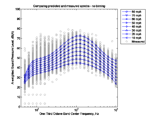
The data in this figure is located here, for Modeled Spectral Content and here, for Measured Data.
Figure 5: Example of Modeled Spectral Content and Measured Data
Two additional questions to consider when modeling REMELs are: "What is the minimum number of samples required?" and "Should data be binned according to speed?" Both of these questions will be discussed in more detail in the following sections, however, a brief review of how these have been handled historically follows.
Historically, data have been computed without binning for computation of the overall A-weighted levels, but have been computed with binning for computation of the spectral coefficients2. Binning should not be used for overall A-weighted levels since confidence intervals rely on the assumption of no error on speed estimates, as discussed in Section 6. Binning is a direct violation of this assumption. Since DE is accounted for in the overall level, binning can be used for the computation of spectral coefficients. The main advantage to binning is that it is more convenient to work with speed-binned spectral data. For large data sets, depending on the analysis software available, it may not be practical to compute spectral coefficients without binning. Specific binning methods are discussed in Reference 2.
Historically, REMELs have been computed with the intention that they be generally applicable to a geographically diverse set of common pavements and vehicles. In order to have reasonable confidence of the estimated parameters for a diverse data set, a relatively large number of samples is necessary. The suggested minimum for general REMELs is given in Reference 5 and is repeated here for convenience.
Speed, mph |
Minimum Number of Samples |
|---|---|
0-10 |
10 |
11-20 |
10 |
21-30 |
20 |
31-40 |
30 |
41-50 |
100 |
51-60 |
200 |
61-70 |
100 |
This document provides additional methods in the next sections for determining if sufficient samples have been obtained. Issues examined relate to the minimum number required for statistical validity, requirements for sufficient speed range coverage, appropriateness of the model, the effect of binning, and tests for statistical significance. By considering the issues explicitly, it may be possible to determine that a smaller data set is sufficient or that a large data set is required.
Identifying and Handling Problematic Data Sets for Overall Levels
The number of samples required and speed range that they should cover depends on a number of factors. At a minimum, there should be sufficient samples such that statistical analysis is valid. As mentioned before speed ranges need to cover the low and high speed ranges. However, when this is not the case, it may be possible to address the issue with substitute data. Finally, it goes without saying that the shape of the REMEL model must be appropriate for the data. REMELs do not allow for curve shapes other than those that can be described by Equation 1 and Equation 3. Several examples of potentially problematic data sets for overall A-weighted levels follow. Each example describes a typical problem and suggests appropriate responses.
Problem 1: Insufficient Data to Obtain Gaussian Estimate of Parameter
The data set is too small if the model parameter estimates are not Gaussian (or nearly Gaussian) in such cases the confidence interval will be artificially larger due to the need to use a t-distribution for confidence intervals rather than a normal distribution6. Fortunately it is expected that the parameter estimates will quickly take on a Gaussian distribution and the shape of the parameter estimate distribution is relatively insensitive to the shape of the data's distribution. For example, when idle data are distributed with a strongly skewed distribution, as in Figure 6, the resultant distribution for C is roughly normal with only 3 samples and is very close to a normal distribution with only 30 samples, as can be seen in Figure 7. (The rule of thumb is that a sample size of 30 is typically sufficient to obtain a normally distributed parameter estimation.) The argument for a normally distributed parameter estimation becomes even stronger for the same number of samples if the underlying data set is itself Gaussian. An example of a Gaussian data set and the corresponding parameter estimate distributions is given in Figure 8 and Figure 9. Here it can be seen that the shape of the parameter estimate quickly approaches normal. It should be noted that normally distributed parameter estimates indicates that statistical analysis based on Gaussian distributions requires a relatively small data set. This does not, however, indicate that there is sufficient data to estimate the parameter within an arbitrary level of confidence. This question is discussed in Section 6. In general it is recommended that at least 30 data samples be collected to assure a reasonably normal distribution when computing overall A-weighted level parameters and that at least 60 data samples be collected to assure reasonably normal distribution when computing spectral parameters7.
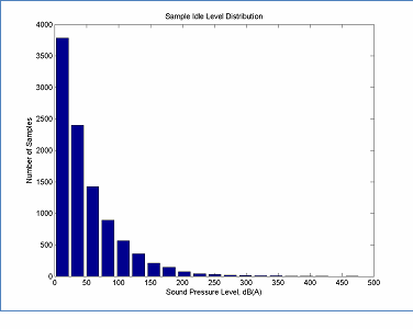
Figure 6: Sample Data Distribution that is Strongly Skewed
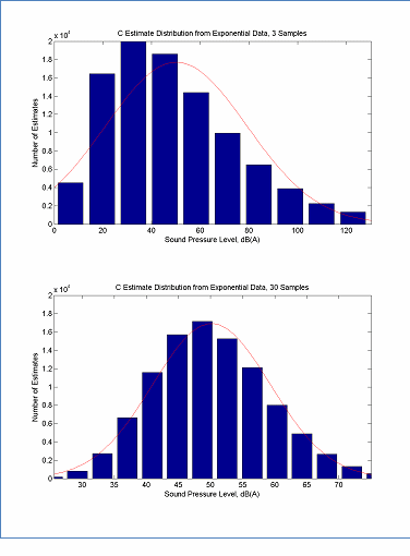
The data in this figure is located here, Estimate Distribution from Exponential Data - 3 Samples and here, Estimate Distribution from Exponential Data - 30 Samples
Figure 7: Distribution of Parameter Estimates for a Strongly Skewed Data Set
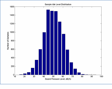
Figure 8: Sample Data Distribution that is Roughly Gaussian
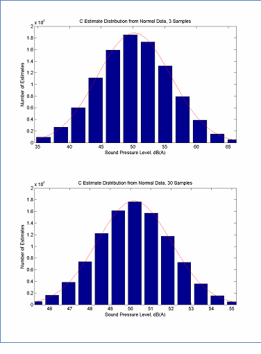
The data in this figure is located here, Estimate Distribution from Normal Data - 3 Samples and here, Estimate Distribution from Normal Data - 30 Samples
Figure 9: Distribution of Parameter Estimates for a Roughly Gaussian Data Set
Problem 2: No Low Speed Data
In the next few examples a simulated data set is used to examine how deficiencies in the sampled data affect the modeled parameters compared to the true curve. In each figure a "true" curve is computed by defining the parameters A, B, and C and computing LA,max for a set of known speeds. "Measured" data is then obtained by adding random noise to the true model. Finally, an "estimated" model is derived by using the "measured" data. If the "true" and "estimated" models are very similar, then the sampled data were sufficient. Figure 10 shows the case where a full set of data were collected and the "true" and "estimated" models match closely.
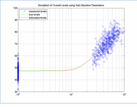
Figure 10: True and Estimated Models ? Full Data Set
If no low speed data are available, as in Figure 11, then the only way to fit all three parameters: A, B, and C with the data set is to use the non-linear form of the model, that is, Equation 1. Even so, the estimated C will not likely match the true model. If a suitable replacement data set can be found, for example if a new pavement is being evaluated for a vehicle type that already has C computed for another pavement, then the pre-computed C can be used. If no equivalent idle data exists, for example a new vehicle with a completely different engine type, then low speed data must be collected to provide a reasonable chance of fitting the low speed range.
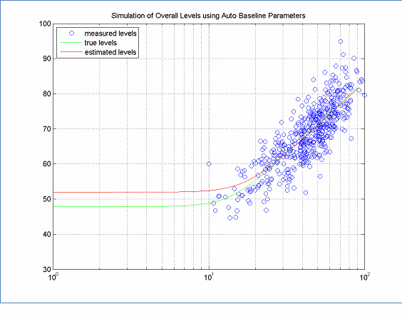
Figure 11: True and Estimated Models ? No Low Speed Data
Problem 3: No High Speed Data
When plotting the data, a key indicator that the high speed data is not high enough is if the high speed data levels are no greater than the random distribution of the low speed data. (Note, you will not be able to evaluate this if you do not have low speed data.) In such cases both A and B coefficients can be significantly off from the true value. This can occur under two conditions: 1) the speed region sampled was not high enough, as in Figure 12, or 2) the vehicle / pavement emissions do not fit the REMEL model. The former will be addressed here, and the latter later. When examining the data, it should become clear if the speeds are not high enough. Since modeling high speed emissions is the primary reason for computing REMELs, higher speed data should be collected until a roughly straight line can be fit through the high speed range. Provided that data can be collected at highway speeds, this problem should not evince itself.
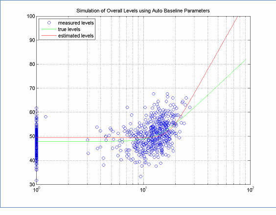
Figure 12: True and Estimated Models ? No High Speed Data
Problem 4: Insufficient Speed Range to Compute High Speed Slope
Another problem that can occur with the high speed data is that there may not be enough range to accurately compute the slope (coefficient A) of the high speed portion of the model. This problem is more likely than not having high enough speeds, since it is possible to measure at one location where all of the vehicles travel at almost the same speed. In such cases, the best solution to this problem is to acquire more data, for example, at other locations along the same highway, at different times of the day or week, on other highways with the same pavement. However, if collecting additional data is not possible, then a substitute A coefficient can be used if it is expected that the level difference between the two REMEL curves is independent of speed in the high speed range. However, it is important to note, that without additional data, it is not possible to check this assumption.
Figure 13: True and Estimated Models ? Not Enough Range on High Speed Data
Problem 5: Data that do not Fit the Model: High Speed Data Extends below Idle
In some cases, the lower end of the high speed data may appear to have lower levels than the low speed data. This can be caused by: 1) using an inappropriate substitute C coefficient, for example using a heavy truck C coefficient when modeling new automobile data; 2) by having insufficient data to accurately model A, B, and C coefficients; or 3) because the underlying data cannot be accurately fit using the REMEL model. There are no known cases in which the model is not appropriate for typical vehicles. Therefore the main recommendations are to make sure that there is enough data to accurately model all parameters.
Problem 6: Data that do not Fit the Model: High Speed Data have No Slope or have Negative Slope
In some cases, there can appear to be a wide enough high speed range but the slope comes out to be either zero or negative. These results, although not mathematically impossible, are not consistent with the expected performance of REMEL modeling. In such cases it is recommended to gather more data, either in the same speed range or over a wider speed range if possible to improve the accuracy of the parameter estimation. With sufficient data it is expected that the slope will be positive.
Identifying and Handling Problematic Data Sets for One-Third Octave Bands
Provided that a sufficient number and range of data have been sampled to compute the overall A-weighted levels, many potential problems with computing spectral REMELs will have been eliminated. However, there are still a few special issues that are related only to spectral REMELs. These include an increased requirement for uniformity in the speed data, issues related to binning of speed data, and issues related to accounting for strong tonal components. An example of a good modeled fit to the spectral data is shown in Figure 14. Even for this model, the fit has some limitations; most notably at low frequencies the model tends to compress the shape of the spectrum. This is not due to deficiencies in the data but to the form of the model, which weights variance at higher frequencies more than at lower frequencies8.
The data in this figure is located here, Spectral Modeling and here, Measured Data
Figure 14: Example with Good Spectral Modeling
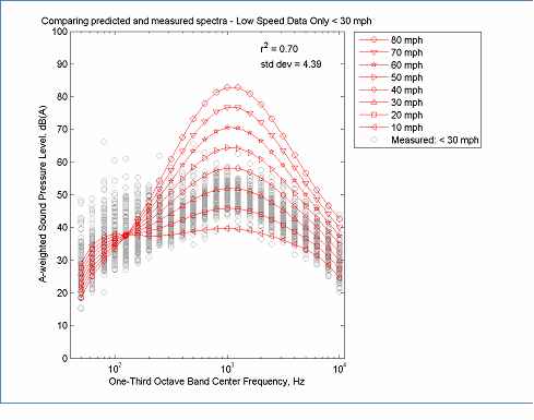
Problem 1: Insufficient Speed Range
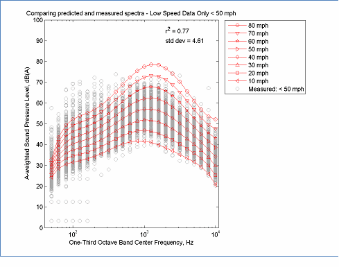
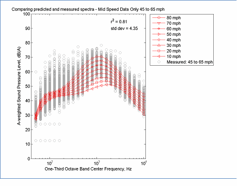
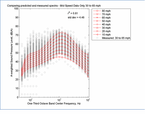
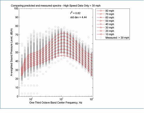
When computing the overall A-weighted level, the REMEL model is a combination of two linear functions. Therefore, when errors are extrapolated, they tend to grow slowly. When computing REMEL spectra, the model is based on a 6th order polynomial of log10(f), therefore extrapolated errors tend to grow quickly. Thus the spectral model is much more sensitive to gaps in the speed distribution of the data. Several examples are shown in Figure 15 to Figure 20. In Figure 15 only low speed data less than 30 mph was used to determine parameter coefficients. When the model was used to extrapolate the spectra at higher speeds, the errors in the mid-frequencies were very large. Although, mathematically realizable, the cross-over at 125 Hz is not typical for averaged spectra. Increasing the minimum speed to 50 mph greatly improves the model, but still results in a greater spread in the spectra than expected from the full data set. The general patterns of these figures indicate that relying on low speed data tends to generate spectra that are "expanded" while relying on high speed data tends to generate spectra that are "contracted" and that the best (data reduced) models occur when the range includes at least the speed range from 30 to 65 mph. Although individual cases may vary, these general observations are expected to provide useful guidance during the evaluation of REMEL spectral results.
The data in this figure is located here, Spectral Modeling and here, Measured Data
Figure 15: Example of Spectral Modeling Using only Low Speed Data < 30 mph
The data in this figure is located here, Spectral Modeling and here, Measured Data
Figure 16: Example of Spectral Modeling Using only Low Speed Data < 50 mph
The data in this figure is located here, Spectral Modeling and here, Measured Data
Figure 17: Example of Spectral Modeling Using only Mid Speed Data ? 45 to 65 mph
The data in this figure is located here, Spectral Modeling and here, Measured Data
Figure 18: Example of Spectral Modeling Using only Mid Speed Data ? 30 to 65 mph
The data in this figure is located here, Spectral Modeling and here, Measured Data
Figure 19: Example of Spectral Modeling Using only High Speed Data > 30 mph
The data in this figure is located here, Spectral Modeling and here, Measured Data
Figure 20: Example of Spectral Modeling Using only High Speed Data > 50 mph
Problem 2: Binning of Data
Although binning of data by speed is not consistent with the assumptions required for computing overall energy means, it is sometimes a practical necessity for computing spectral REMELs. Comparing the binned results from Figure 21 and Figure 22 with the original un-binned results Figure 14, it can be seen that modeling process is much less sensitive to binning than incomplete speed ranges, however, it can also be seen that low frequencies are compressed even more with binned data than with the original data. Also, the process of binning can upset the weighting of speeds based on sample size (although binning schema can be selected to weight one speed range more than others.) In general, if there is not a practical expediency to binning speed data, it is recommended to not use binning.
Note, the improved r2 values for binned data are due to the aggregation of data, but do not provide improved confidence intervals since they decrease the effective sample size.
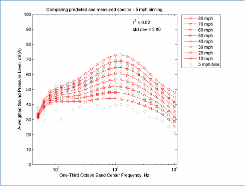
The data in this figure is located here, Spectral Modeling and here, Measured Data
Figure 21: Spectral REMELs Derived from 5 mph Speed Bins

The data in this figure is located here, Predicted data and here, Measured Data
Figure 22: Spectral REMELs Derived from 10 mph Speed Bins
Problem 3: Strong Tonal Components
One final problem associated with REMEL spectral models is the handling of data with strong tonal components. These components can be present, for example, for pavements with periodic transverse patterns, such as transversely tined PCC. The problem with tones is that they generate an abrupt change in level from one band to the next; however, the spectral model does not have a high enough order to account for these abrupt changes. An example is given in Figure 23. Here a tonal component is present in the 400 Hz one-third octave band that is 10 dB above the adjacent one-third octave bands, however there is no noticeable difference in the spectra from one without the tonal component present. This illustrates that REMELs alone are not well suited for modeling tonal components. One method to handle these tones would be to provide a frequency specific correction for tonal components, such as has been done for OBSI modeling.
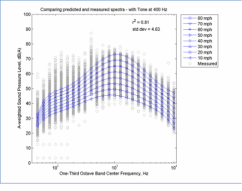
The data in this figure is located here, Predicted data and here, Measured Data
Figure 23: Example of REMEL Spectra and Underlying Data with Tonal Component
Evaluating Significance
A data set can produce results that do not show any anomalies in the shape of the curve or how it fits the data, however, unless the confidence interval for the model is evaluated, it cannot be said that enough data has been sampled in order to distinguish the new curve from existing curves, or that new curve represents the new vehicle or pavement type within a desired tolerance. The only way to assure that enough data has been sampled is to compute confidence intervals. The discussion that follows assumes that the model parameters capture the deterministic character of the data and that all variance not captured by the parameters is due to random factors associated with either measurement of the sound level or site-to-site variation. It is assumed that the parameter estimates are normally distributed. In this section, two confidence intervals will be developed. The first is useful for determining if enough data have been collected in order to provide a tolerance on the model, that is, the REMEL curve is within N dB of the true energy mean curve for the vehicle / pavement combination. The second confidence interval is useful for comparing a new curve with others to determine if the new curve is significantly different. If a new curve is not statistically different from an existing curve, then any interpretations based on the new curve that are not consistent with interpretations based on the old curve are highly questionable.
In general we can test whether sufficient data have been acquired by computing a confidence interval as follows:
Computation of the REMEL model has already been discussed. Variance is modeled by expanding Equation 5 .
Equation 5: General Equation for Variance
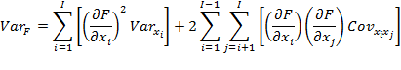
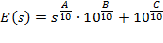
where, F is given by
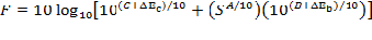
that is, the energy averaged overall A-weighted level. Using these two equations, the specific variance for F can be determined using Equation 6
Equation 6: Total Variance
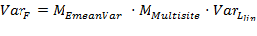
where,
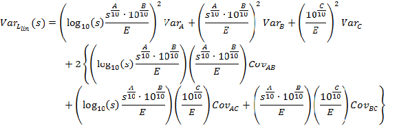
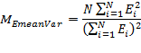
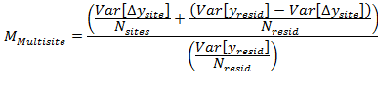
A, B, C, VarA, VarB, VarC, CovAB, CovAC, and CovBC should be determined as part of the curve fitting process for the overall A-weighted level. The correction for the energy mean is simply the number of data samples multiplied by the sum of the individual data samples' energy squared divided by the square of the sum of the individual data samples' energy. The multi-site correction is a little more complicated because the variance must be separated into the portion related to sample-to-sample variation and the portion related to site-to-site variation. The site-to-site variation is estimated using the mean values for each site. The sample-to-sample variation is then computed as the total variation minus the site-to-site variation. Each component of variation is then weighted by it respective number of samples. Since the number of residuals is equal to the number of samples Nresid is used for both the total variance and for the sample-to-sample variance. Further details on the derivation of this specific expansion of Equation 6 can be found in References 3 and 4.
Once the variance has been determined, it is a simple matter to determine the z-score required to produce the appropriate interval. It is suggested that a 95% confidence interval be used when evaluating if the tolerance on the curve estimation is sufficiently small. Here one wants a high degree of confidence, since a false conclusion will result in an incorrect estimation. It is suggested that a 50% confidence interval be used when evaluating whether two curves are different. Using a 50% confidence interval will increase the likelihood of accepting the alternate hypothesis that the two curves are different, however, it is assumed that there is already significant evidence to indicate that there is a difference, otherwise the measurements would not have been made in the first place. (If the primary reason for conducting the measurements is not based on some anecdotal evidence that the vehicle / pavement is indeed different, then a 95% confidence interval is recommended for both types of tests.)
Figure 24 provides an example of the confidence interval computed for a large data set. Note that the interval is wider at low speeds than at high speeds. This is because there were a large number of samples at high speed, causing those parameters that control the curve at high speed to have low variance. Since the variance model is a function of speed, the change in total variance is captured. By evaluating the confidence interval over its entire range, one can determine not only if more data are needed in general, but in what speed range. Note that this is also partly a design consideration. If low speed modeling is not required, then a broader confidence interval can be tolerated at low speeds.
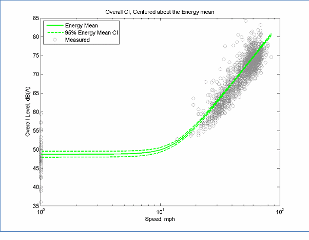
The data in this figure is located here, Measured data and here, Mean Data
Figure 24: Measured Data, REMEL Curve, and Confidence Interval for Large Data Set (TNM Auto Baseline)
Figure 25 shows two hypothetical curves that are being compared to determine if they represent two unique curves or if they represent different samples from the same population. Even though the data have significant overlap, the curves have a level difference of 3 to 5 dB. However, even when requiring a confidence of only 50%, these data do not support the use of two curves. Assuming that the data are from different populations, gathering more data may decrease the confidence intervals such that it can be concluded that they are unique curves with sufficient confidence. Note also, that curves do not need to be unique at all speeds. In many cases, the low speed portion may be sufficiently similar that no conclusion of uniqueness can be made with confidence, however, if the high speed data are unique, then the whole curve should be considered unique.
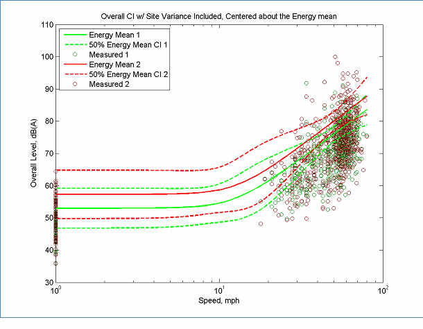
The data in this figure is located here, Energy Measured 1 data and here, Energy Measured 2 Data and here, Energy Mean 1 data and here, Energy Mean 2 Data
Figure 25: Confidence Intervals for Two Curves. Are they Statistically Different?
Any many cases, it will be desired to determine if a new curve is unique compared to the existing curves used by TNM. In such cases, the multipliers for the TNM curves are required. These were developed by Grant Anderson6 and have been included here for convenience.
TNM Vehicle Type |
MMultisite |
|---|---|
Automobile |
31.6 |
Medium Truck |
4.8 |
Heavy Truck |
17.8 |
Bus |
2.0 |
Motorcycle |
4.8 |
The discussion of statistical significance has focused on the REMEL overall A-weighted level curve. Even for this simple, three-parameter model the derivation for the total variance is reasonably involved. The development of the total variance for the spectral model is beyond the scope of this document. Further, since this variance would be a function of both speed and frequency, it would require a two-dimensional model, which would be difficult to visualize and interpret consistently and meaningfully. It is suggested that the most practical statistical metrics for the spectral model are the r2 value and the mean-squared-error. These metrics will allow one to evaluate if one model is better than another for the same sampled data, but not to distinguish different populations.
Summary and Sample Implementations
The steps below outline the general approach for computing REMELs using a small dataset:
A. Overall (Broadband) Levels
B. One-third Octave Band Spectra
This approach relies on comparing the results against required levels of confidence in order to determine if enough data have been collected. Although 30 samples may be sufficient in some cases, it should be expected that in many cases several hundred samples may be required.
If a full set of data are available for a vehicle – pavement combination, then all terms can be determined. If there is no idle data, then C and DEc cannot be determined from the data and an existing vehicle – pavement pair must be identified for use as a substitute. When determining coefficients A, B, and C. The resulting curve should be plotted with the data as a first analysis of the quality of the fit. If the slope is zero or negative, or if the mid speed data seems to dip significantly below the mean low speed level, then it is likely that more data are needed. If the curve fits the data well, then confidence intervals should be developed to determine if the curve is known within a required tolerance and, if intended to replace another curve, it should also be compared against the previous curve. Spectral modleing should be done with a speed range from low to high in order to anchor the spectral coefficients. If there is insufficient spectral data, then more should be gathered. If this is not practical, replacement data may need to be generated from a suitable donor model.
Figure 26 shows confidence intervals for three sets of automobile data with similar pavement types. REMELs 1995 – Autos, DGAC is a model used by TNM 2.5, REMELs Light – Autos, DGAC is a model developed from two measurements in Massachusetts, REMELs Light – Autos, RAC is a model developed from two measurements in Arizona and one in California. Because the REMELs Light data only have data in the mid- to high-speed range, the confidence intervals at low speed are not of interest here. At high speeds, there is at least some separation, however, this figure illustrates one more "sample size issue" with which to be cautious. The site-to-site variance for the Massachusetts data was small. Because there were only two sampled sites, it is very likely that by chance the two estimated site means were very close. In order to have any useful confidence in the site-to-site variance, one should measure at the very least three sites, however, five to ten would be much more reasonable.
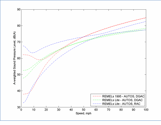
The data in this figure is located here, REMELs 1995 - AUTOS, DGAC and here, REMELs Lite - AUTOS, DGAC and here, REMELs Lite - AUTOS, RAC
Figure 26: 50% Confidence Intervals for Three Sets of Modeled Data

