
The Federal Highway Administration (FHWA) released Traffic Noise Model (TNM) 1.0 in 1998 as the new generation of highway noise modeling software for use on Federal-aid projects. The FHWA has updated the software on several occasions since the initial release, with the last major update in 2004 to the current version 2.5 (version 3.0 is expected to be released in 2016). The FHWA TNM has been shown to be quite accurate for the prediction of highway traffic noise, as demonstrated by FHWA's multiple-phased model validation study that began in July 1999 and continues to this day.[1] With the release of FHWA TNM version 2.5 in 2004, the tendency of earlier versions of the FHWA TNM to over-predict noise levels at moderate to large distances over hard ground was addressed.[2] While the FHWA TNM provides for the accurate prediction of traffic noise levels along the wayside of a highway, accurate results are not necessarily guaranteed. Accurate results depend upon the quality of the input data and the care with which the user replicates objects in the physical world with objects in the virtual world of the FHWA TNM.
The FHWA provides guidance and advice on the use of the model through its webpage[3] and supporting documents, such as the FHWA TNM User's Manual, and through training courses offered by the National Highway Institute.[4] These resources provide users with basic knowledge and guidance for the routine application of the FHWA TNM for the prediction of highway traffic noise. In recognition that user practices for the input of TNM objects vary, the FHWA has undertaken additional studies to provide additional guidance and recommended best practices for special scenarios that run somewhat outside the routine application of the model. The recently released National Cooperative Highway Research Program (NCHRP) Report 791 provides recommended best practices and analysis techniques for modeling scenarios that range from structure-reflected noise to tunnel-radiated noise.[5] Although that document provides much needed guidance, it does not identify the best sources for input data or how to find the additional information that is critical to the development of an accurate model of highway traffic noise. As a result, the FHWA has undertaken the current study that builds upon the work in the prior projects, so that collectively the entire body of work will provide a comprehensive set of Best Practices for the use of the FHWA TNM.
The TNM objects that describe the project geometry are familiar to TNM users and include roadways, receivers, noise barriers, rows of buildings, terrain lines, ground zones, and tree zones. An accurate model of highway traffic noise depends upon the accuracy with which users code the horizontal and vertical geometry of the project.
More often than not, project geometry within the right-of-way is developed with a high level of accuracy and is often based on survey data. Horizontal and vertical geometry are provided in the form of roadway plans, profiles, and cross-sections. While survey data always are available for highway design studies, survey data may not be available for planning studies. As a result, TNM users must find their own sources for geospatial and elevation data in these cases.
In addition, the high-quality elevation data that are developed for highway projects and based on surveys usually have limited coverage for the purposes of highway noise analysis. That is, the survey data often are limited to areas that are within the highway's existing and/or proposed right-of-way. However, highway noise analysts require geospatial and elevation data to predict traffic noise levels in the communities adjacent to highway corridors, often at distances of 500 to 1,000 feet from the project roadways. For this reason, TNM users may need to supplement the project's survey data with geospatial and elevation data from third-party sources.
The use of high-quality geospatial and elevation data is just one requirement for producing accurate results from the FHWA TNM. Before identifying sources of high-quality geospatial and elevation data, the next section provides an overview of the industry's current best practices and guidance related to topography.
Tip: Do not use the lines that comprise a triangular irregular network (TIN) to digitize or create terrain lines in the FHWA TNM. The TIN is the framework used to connect elevation points. A TIN is a derivative product that can be used to create topographic contours. Users should use topographic contours to guide the creation of terrain lines in the FHWA TNM.
NCHRP Report 791 Chapter 8 provides guidance on the use of geographic features within the FHWA TNM, including best practices associated with locating the outside edge of pavement (or “equivalent” terrain line) in the horizontal plane, placing terrain lines along elevated roadways, minimum spacing for terrain lines, vertical precision for terrain lines and barrier tops, and modeling of flat-top earthen berms. It is worthwhile to highlight some of the key findings of NCHRP Report 791 that pertain to these topographic objects in the FHWA TNM.
TNM users should review NCHRP Report 791 Chapter 8 and the supporting details in Appendix G of that report to increase their understanding of the FHWA TNM's sensitivity to the vertical precision of the modeled geometry. Based on the recommendations of NCHRP Report 791, it is clear that TNM users require high-quality topographic data to ensure the accurate prediction of highway traffic noise levels and design of noise barriers. The next sections provide an overview of the National Spatial Data Infrastructure and the different types of elevation data that are available.
The Federal Geographic Data Committee (FGDC) is a 32-member interagency committee with representatives from the Executive Office of the President, along with Cabinet-level and independent Federal agencies. It was established in 1990 to promote “the coordinated development, use, sharing, and dissemination of geospatial data on a national basis.” This nationwide effort is known as the National Spatial Data Infrastructure (NSDI) and is hosted by the U.S. Geological Survey (USGS).[6]
The NSDI is made up of a number of connected elements ranging from clearinghouses, catalogs, and portals, to metadata, framework data, and standards. Other elements of the NSDI include collaborative partnerships between diverse sets of stakeholders and public policies that promote a number of goals including public access to and sharing of data. One of the core elements of the NSDI is the development of standards for geospatial data and technology. FGDC-endorsed standards are required for use by Federal agencies.[7] At least one state highway agency (SHA) has adopted FGDC standards as recommended practice.[8] The NSDI Framework is comprised of seven themes of data designated as:
In 2014, the USGS published Circular 1399 “The 3D Elevation Program Initiative - A Call for Action”[9] as a means to achieve an overarching goal, which is to accelerate the collection of three-dimensional (3D) elevation data, in an attempt to completely refresh the National Elevation Dataset with new elevation data products and services on a nationwide basis, in a period of 8 years. This report summarizes some of Circular 1399's findings in a later section, focusing on the findings related to the existing coverage of elevation data for a given quality level. Circular 1399, Appendix 1 provides detailed definitions for different types of source data, elevation models, and derivative products.
“Source data” are the raw data for elevation models and other derivative products (e.g., contours, cross-sections, profiles, etc.). Examples of source data include:
The most familiar derivative product of the models list above is a set of topographic contours, or lines of equal elevation on the Earth's surface. Another type of derivative product is a triangulated irregular network (TIN). A TIN is a vector-based representation of a land surface, made up of irregularly distributed nodes and lines with 3D coordinates creating a network of triangles.[10]
TNM users should be aware that there are many different types of elevation datasets; some much older than others. The datasets and types of data listed above represent some of the more recent/common types of elevation data in use today. TNM users can find standard definitions and more details about the types of elevation datasets available to the public by searching the internet for the type of dataset.[11]
Having introduced some terminology and concepts related to geospatial data, the next section identifies sources of high-quality data for use in highway noise studies.
A wide range of geospatial data exists in a variety of clearinghouses, catalogs, and portals, hosted by a broad range of partners/stakeholders, including various Federal, state, local, and tribal governments through their agencies, as well as academia and the private sector. This study does not include a catalog of all sources for geospatial and elevation data; however, the study team identified a source of high quality data elevation data available to the public and provided examples of other reliable sources of data from state governmental agencies. See the end of this chapter for tips for conducting a search for other geospatial and elevation data.
The National Map is a collaborative effort among the USGS and other Federal, state, and local partners to improve and deliver topographic information for the nation. The National Map contains a broad range of geospatial data and information including: orthographic images, elevation, geographic names, hydrography, boundaries, transportation, structures, and land cover.[12] Research conducted in support of this study indicates that a number of SHAs and their consultants rely on The National Map for geospatial and elevation data for highway noise studies.[13]
For more than 15 years, the USGS has offered a variety of elevation data products and services through the National Elevation Dataset (NED), which was the elevation layer for The National Map. The USGS derived the NED from diverse source datasets processed to a specification with consistent resolutions, coordinate system, elevation units, and horizontal and vertical datums (refer to Table I-1). Elevation data contained within the NED were typically represented as topographic contour lines and bare earth DEMs. In 2015, the USGS incorporated new sources of elevation data (LiDAR and Ifsar) into The National Map through the 3D Elevation Program (3DEP) initiative. As a result of the transition to 3DEP, the USGS now provides source LiDAR point clouds, Ifsar DSMs, and orthorectified radar intensity images (ORIs) over certain areas of the country.[14] The data holdings of the NED have been incorporated into the 3DEP, and as a dataset and system, the NED has been retired.[15]
Source: Gesch, D., Evans, G., Mauck, J., Hutchinson, J., Carswell Jr., W.J., 2009, The National Map-Elevation: U.S. Geological Survey Fact Sheet 2009-3053, 4 p.
Figure I-1 shows a screen-shot of The National Map Viewer and Download Platform,[16] which allows visualization and download of the most current topographic base map and products free of charge. Various data themes of geospatial data are available for download, including: boundaries (National Boundary Dataset), elevation products (3DEP), elevation source data (3DEP), hydrography and watersheds, imagery (1-foot), imagery (1-meter), map indices, geographic names (Geographic Names Information System), structures (National Structures Dataset), transportation (National Transportation Dataset), and woodland tint.
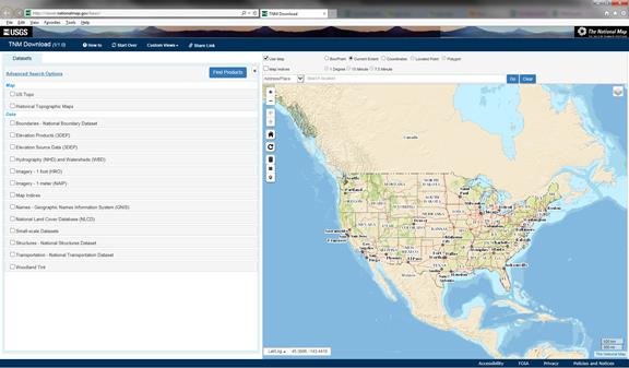
Source: https://viewer.nationalmap.gov/basic/.
Figure I-1. The National Map Download Client (v1.0)
The next section provides background on the 3DEP initiative and insight into the ongoing development of the elevation dataset layer in The National Map.
As discussed in USGS Circular 1399, the 3DEP initiative serves to accelerate the collection of 3D elevation data and update the NED with new elevation data products and services within an 8-year timeframe. The initiative strives to replace elevation data older than 30 years old, on average, with newly created elevation data derived from LiDAR and Ifsar technologies. The success of the initiative depends upon a number of factors, not the least of which is the participation of cooperating agencies from Federal, state, and tribal governments.
Figure I-2 (taken from USGS Circular 1399) serves to illustrate the current task. It shows a map of the U.S. with the status of the NED as of May 2014. It shows that elevation data (DEMs) based on LiDAR technology is available for only 26 percent of the conterminous United States (CONUS), Hawaii, and U.S. territories, while Alaska has DEMs based on Ifsar technologies covering 37 percent of the state. The aforementioned rates of coverage are for DEMs obtained from LiDAR and Ifsar datasets covering the full range of Quality Levels.[17] The goal of the 3DEP initiative is to obtain full coverage for the CONUS at a Quality Level of 2 or better by 2022. As of the publication of USGS Circular 1399, only 4 percent of the CONUS, Hawaii, and U.S. territories had LiDAR data that met the desired Quality Level.
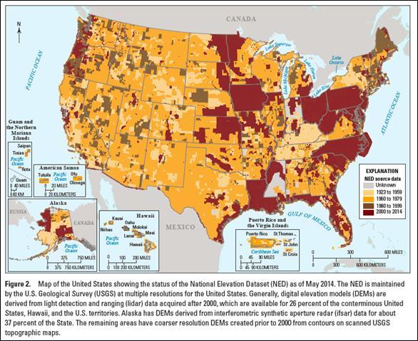
Source: USGS Circular 1399
Figure I-2. Status of the National Elevation Dataset (NED) as of May 2014
Clearly there is still work to be done if the USGS and its cooperating agencies are to meet the goals of the 3DEP initiative. Nevertheless, based on the progress made to date, the study team believes that The National Map and the 3DEP dataset are a reliable source for high-quality geospatial and elevation data. If the goals of the 3DEP initiative are met, The National Map will very likely represent the largest collection of high-quality elevation data for the CONUS, Hawaii, U.S. territories, and Alaska.
A broad range of partners and stakeholders including various Federal, state, local, and tribal governments through their agencies, as well as academia and the private sector, provide geospatial and elevation data through a variety of clearinghouses, catalogs, and portals. The National Map Viewer and Download Platform is one example of a clearinghouse for geospatial and elevation data. The study team conducted research to identify what other sources of geospatial and elevation data may be available from agencies at other levels of government. Additionally, the study team obtained information from the Transportation Research Board (TRB) Committee ADC-40 on Transportation-Related Noise and Vibration and the American Association of State Highway Transportation Officials (AASHTO) Noise Work Group about sources of geospatial and elevation data used by participating SHAs.
Table B-1 in Appendix B contains a list of sources for geospatial and elevation data used by various SHAs across the country provided by TRB ADC-40 and the AASHTO Noise Work Group. Table B-1 shows information provided by SHAs from Florida, Kansas, Massachusetts, Montana, New Hampshire, Ohio, Tennessee, Virginia, and Washington.
Many states, such as Massachusetts, have independent departments or offices that coordinate activities within the state. MassGIS is the Commonwealth's Office of Geographic Information, within the Massachusetts Office of Information Technology of the Administration and Finance Secretariat. The Massachusetts Legislature established MassGIS as the official state agency assigned to the collection, storage, and dissemination of geospatial data.
Table B-2 in Appendix B contains additional sources of geospatial and elevation data obtained by the study team through a series of systematic searches on the internet, using official state websites as a starting point in each case. The online searches indicated that in a few cases, SHAs are sources of geospatial and elevation data within a state. In other cases, a state's Department of Natural Resources is a source of geospatial and elevation data.
Table I-2 provides a brief listing of additional sources for geospatial data.
Environmental Systems Research Institute (ESRI) |
http://www.esri.com/data/find-data (ESRI is an international supplier of GIS software and applications. ESRI products are available at different levels of licensing. Access to GIS content on the ESRI website requires an online subscription.) |
|---|---|
Open Topography |
OpenTopography is supported by the National Science Foundation under Award Numbers 1226353 & 1225810 http://www.opentopography.org/index.php |
USDA Geospatial Data Gateway (GDG) |
|
US Census Bureau TIGER/Line® Shapefiles and TIGER/Line Files |
|
USGS Earth Resources Observation and Science (EROS) Center |
TNM users may be faced with the possibility of having to conduct an online search for geospatial data - especially if they are working on a highway project in a region unfamiliar to them. Below are tips for conducting such searches.
Geospatial data are available in a range of formats. If data are not available in the preferred format, be prepared to convert the data to other formats, as needed. Most GIS- and CAD-based applications can handle a range of data formats and can convert data from one format to another.
This section identifies best practices for dividing traffic volumes and vehicle mixes across roadways with multiple lanes. In developing the best practices, the study team modeled a variety of scenarios to test for changes in calculated TNM sound-level results attributable to changes in traffic distributions across multiple lanes. The study team used the FHWA TNM to model 4-, 8-, and 12-lane limited access highway facilities and tested the sensitivity of TNM-calculated sound levels to a non-uniform distribution of vehicle volumes / mixes across multiple lanes. As detailed in a later section, the study team derived a typical non-uniform traffic distribution from traffic counts obtained by the Volpe Center during the Phase 1 TNM Validation Study. This research compared TNM sound-level results for the non-uniform traffic distribution to a reference case with even distribution of vehicle volumes and mixes across all lanes of travel. Additional scenarios tested the sensitivity of the FHWA TNM to traffic data input (volume, mix, and speed), focusing on Level of Service (LOS) based approaches compared to approaches using design hourly volumes.
Before describing the process used to develop the recommended best practices, the following section reviews the status of the current best practices related to modeling multiple-lane highways in the FHWA TNM.
NCHRP Report 791 Chapter 6 provides guidance and recommendations related to modeling techniques for multiple-lane highways using the FHWA TNM. The evaluation of the candidate modeling techniques included comparisons of modeled sound-level results to measurement data obtained by the Volpe Center as part of the Phase 1 TNM Validation Study. The study evaluated three modeling techniques to account for the effects of the roadway shoulder and the “outer” diffracting edge created by the edge of pavement and/or the edge of the shoulder and considered the effects of grouping the lanes on a multiple-lane highway as an alternative to modeling individual lanes. It is worthwhile to highlight some of the key findings of NCHRP Report 791 Chapter 6:
The above best practices were based upon the calculated TNM sound-level results for a “generic” project, consisting of a 4,000-foot long divided highway with a level grade, a paved median and shoulders, with directional volumes of 2,000 automobiles, 200 medium trucks, and 200 heavy trucks, all traveling at a speed of 60 miles per hour (mph). The individual-lane scenarios considered an even distribution of traffic volumes across multiple lanes of travel.[20]
This study built upon the best practices described in NCHRP Report 791 and examined the effects of a non-uniform traffic distribution across a multiple-lane highway. The next section describes the steps taken to develop a “typical” non-uniform traffic distribution for use in the evaluation.
This analysis required traffic distribution across lanes for 4-, 8-, and 12-lane highways for all traffic and by vehicle class. Traffic distribution has significant local variability, and traditional sources such as the “Highway Capacity Manual (HCM)” do not discuss this issue in sufficient detail.[21] The study team used the volume counts collected by the Volpe Center for the Phase 1 TNM Validation Study to derive the needed traffic distributions. These data consist of actual 5-minute volume counts collected at eight 4-lane highway locations, nine 8-lane highway locations, and two 12-lane highway locations that include six, one, and zero rural locations, respectively, with the balance being conducted in urban areas. These volume counts classify vehicles as auto, medium truck, heavy truck, bus, or motorcycle. The study team judged these data as the best available set of data for the objectives of this study.
Conducting the analysis required determination of traffic distributions for each 5-minute time interval. The first step in this process required determining the distribution of several grouped vehicle classes by lane for each time interval. These groups included: auto and motorcycle; medium truck and bus; heavy truck only; medium truck, heavy truck, and bus; and all vehicle classes. The next step involved averaging these distributions for each highway across all time intervals to develop representative traffic distributions of each vehicle class group for 4- and 8-lane highways (urban, rural, and overall) and 12-lane highways (urban only). For example, for a rural 4-lane highway, the representative traffic distribution indicates that 59 percent of autos and motorcycles are in the outside lane and 41 percent are in the inside lane, with similar values available for the other highway types and vehicle class groups mentioned.
The study team also examined traffic distributions for 4- and 8-lane highways for facilities with lower and higher truck volumes and used truck percentages on the 4-lane highways (7-34%) and 8-lane highways (6-19%) to identify the facilities as having lower or higher truck volumes. Next, the team determined representative traffic distributions for the same vehicle class groups listed above for 4- and 8-lane highways with lower truck volumes (average of 10% and 8% trucks, respectively) and higher truck volumes (average of 29% and 16%, respectively). As a point of reference, the “2013 FHWA Freight Facts and Figures”[22] references 4.3 percent and 25 percent as a typical and a high truck percentage, respectively.
Finally, the study team determined traffic distributions needed to simulate rural and urban 4- and 8-lane highways with zero trucks in the vehicle mix. To do this, the team applied the HCM passenger car equivalent (PCE) conversion factor of 1.5 to the truck vehicle classifications in the Volpe dataset and summed these new volumes by lane for each time interval, and for each time interval the proportion of traffic for each lane was calculated and averaged across all time intervals to derive a representative traffic distribution for 4- and 8-lane highways without trucks.
The two 12-lane highways in the Volpe dataset each have managed high-occupancy vehicle lanes. However, it was desirable to derive a representative traffic distribution for a 12-lane facility that was all general-purpose lanes. Because the innermost lane will generally have lower traffic volumes, data from the fifth lane was used to derive an estimate. Rather than simply duplicate the values from the fifth lane, new values were derived for the fifth and six lanes by multiplying the original volumes for the fifth lane by 1.1 and 0.9, respectively.
Appendix C summarizes the traffic distributions derived from the Volpe data in tabular format. The traffic distributions in the appendix provide the basis for the test cases described in the next section.
Finally, the HCM and AASHTO's Green Book[23] provided representative LOS and speed values for rural and urban 8-lane highways, as shown in Table I-3. The speeds in the table are those used to conduct additional TNM sensitivity analyses for the 8-lane scenario.
Source: Based on the Highway Capacity Manual, 2000
Notes: ADT = average daily traffic.
In developing the scenarios to test the FHWA TNM's sensitivity to a non-uniform traffic distribution, the study team followed the NCHRP Report 791 best practices for multiple-lane highways as a starting point. In particular, the scenarios made use of dummy lanes to model the outer and inner shoulders of each multiple-lane highway. Each scenario also provided 0.1-foot overlaps between adjacent travel lanes and between travel lanes and shoulders, along with a 10-foot median. Each “test” scenario for a non-uniform traffic distribution was compared to the reference scenario, which simply consisted of a uniform vehicle distribution across the lanes of travel.
In developing the modeling scenarios, the study team focused on the distribution of traffic across general-purpose lanes and did not include high occupancy vehicle (HOV) lanes, collector-distributor roads, or ramps. Traffic volumes and vehicle mixes for these other types of travel lanes typically originate from the traffic study for a highway project. TNM users do not routinely develop traffic data for such types of travel lanes.
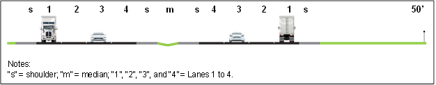
Figure I-3 shows the cross-sectional geometry for the 4-lane at-grade highway configuration along with the lane designations used in this study. Following the convention shown in the figure, Lane 1 is the outermost lane or the rightmost lane in the direction of travel. Lanes 2 to 4 are additional travel lanes located to the left of Lane 1, when in the direction of travel. Figure I-3 also shows the locations of the shoulders (“s”) and median (“m”), as well as the 5-foot receiver at a distance of 50 feet from the near lane of travel.
The modeled scenarios are described as follows:
Figure I-4 shows TNM cross-section views of the modeled geometry for each of the three scenarios developed for a 4-lane highway facility: (i.) highway at-grade; (ii.) depressed highway; and (iii.) elevated highway.[24] Note that the 4-lane highway is configured from left to right in the figure, as follows:
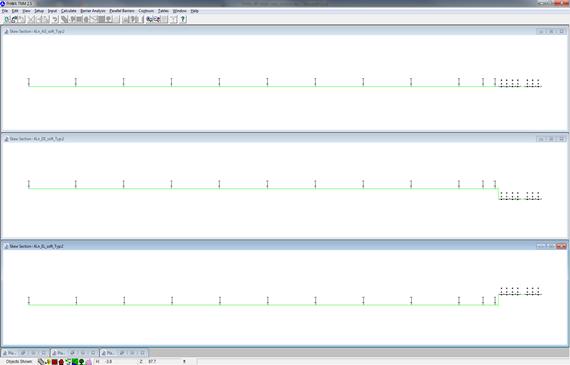
Figure I-4. TNM Cross-section Views showing the Modeled Geometry for the 4-lane Facility
Table I-4 shows the non-uniform traffic distributions used in the scenarios for the 4- and 8-lane highways, while
Table I-5 shows the traffic distributions for the 12-lane highway. These distributions were based on an analysis of the traffic data that were collected by the Volpe Center for the Phase 1 TNM Validation Study.
Figure I-5 through Figure I-8 present the effects of a non-uniform traffic distribution on TNM-calculated sound levels. The graphs summarize the sound-level differences between the uniform and non-uniform traffic distributions for 4-, 8-, and 12-lane highway facilities with cross-sectional geometries that are at-grade (“AG”), depressed (“DE”), and elevated (“EL”). FHWA TNM version 2.5 calculated all results depicted in Figure I-5 through Figure I-8. The following observations are made about the effects of a non-uniform traffic distribution for a multiple-lane highway:
Appendix D includes tabulated sound-level results for all of the scenarios depicted in Figure I-5 through Figure I-8.
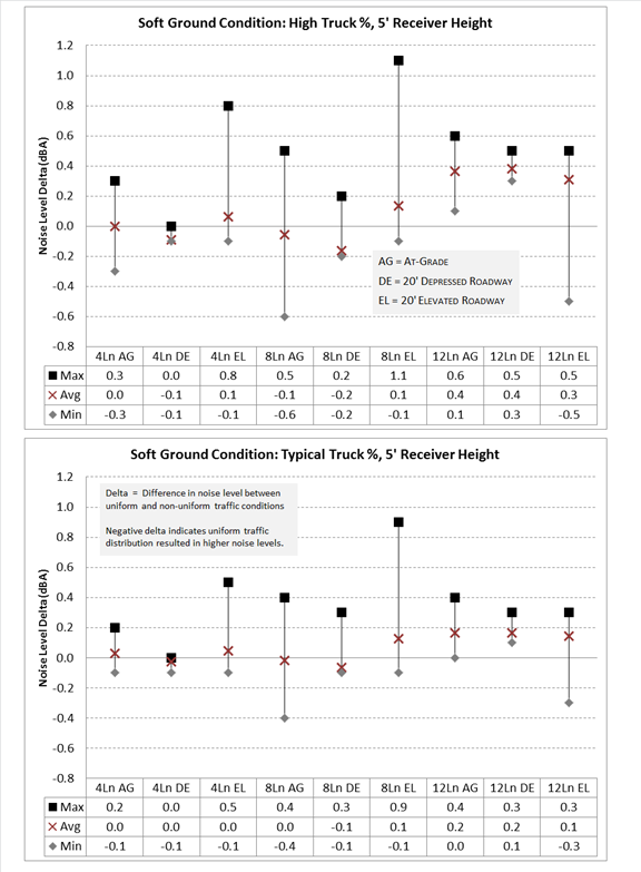
Figure I-5. Effects of a Non-uniform Traffic Distribution for Soft Ground and 5-foot Receiver Height
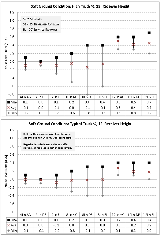
Figure I-6. Effects of a Non-uniform Traffic Distribution for Soft Ground and 15-foot Receiver Height
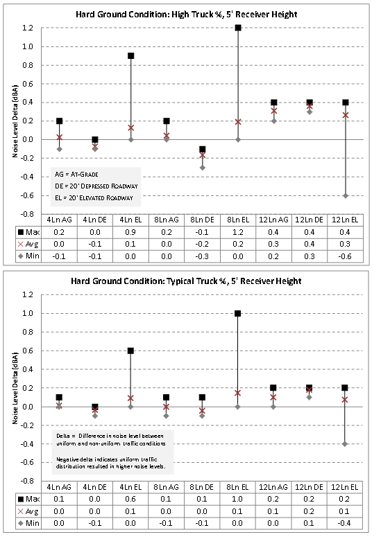
Figure I-7. Effects of a Non-uniform Traffic Distribution for Hard Ground and 5-foot Receiver Height
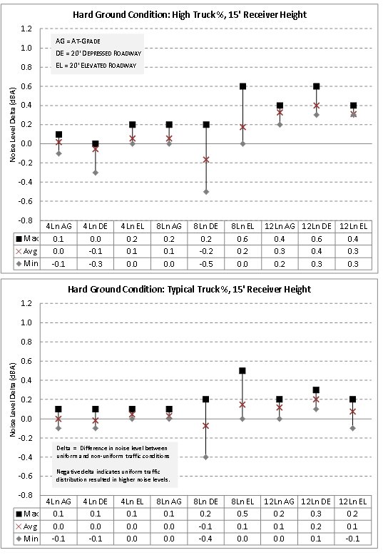
Figure I-8. Effects of a Non-uniform Traffic Distribution for Hard Ground and 15-foot Receiver Height
The calculated sound-level results summarized in the previous section came from scenarios modeled in FHWA TNM version 2.5. The study team also used a beta version of FHWA TNM 3.0 to check the consistency of its sound-level results with version 2.5 and found that the effect of a non-uniform traffic distribution using FHWA TNM 3.0 resulted in a close match with the effect using FHWA TNM 2.5, as demonstrated by the graphs of Figure I-9 and Figure I-10 for a 12-lane facility. While the figures show very good agreement between version 2.5 and 3.0, note that the “effects of non-uniform traffic distributions” show the difference between TNM-calculated sound levels for a non-uniform case and a uniform traffic distribution. The study team noted poor agreement when comparing the absolute sound levels calculated by each model for sound propagation over soft ground. In general, FHWA TNM 3.0-calculated sound levels lower than FHWA TNM 2.5-calculated sound levels by up to 8 dB, or approximately 2.6 dB, on average. Absolute sound levels calculated with FHWA TNM 3.0 showed better agreement with FHWA TNM 2.5 for sound propagation over hard ground. FHWA TNM 3.0 sound levels ranged from 0.4 to +0.3 dB relative to FHWA TNM 2.5 sound levels.
Testing with FHWA TNM 3.0 evaluated only the 12-lane scenarios. The study team expects similar results would be obtained for the 4- and 8-lane scenarios.
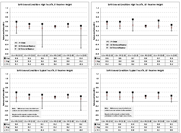
Figure I-9. Comparison of TNM 3.0 and TNM 2.5 Results for a 12-lane Highway over Soft Ground
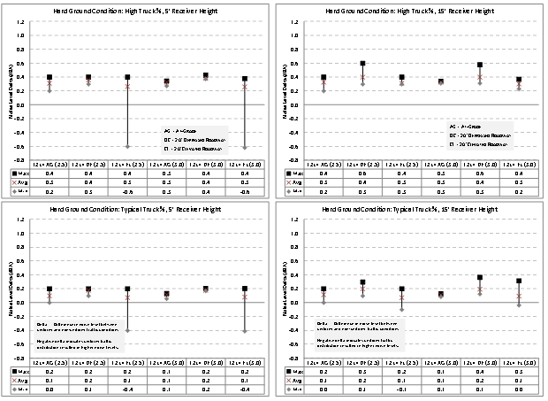
Figure I-10. Comparison of TNM 3.0 and TNM 2.5 Results for a 12-lane Highway over Hard Ground
TNM users often face the task of identifying sources of traffic data, or even developing traffic data for use as input to the model, most often during the planning stage of a highway project. Typical forms of traffic data used to approximate traffic conditions for the loudest hour of the day include design hourly volumes (DHV) and speeds, level-of-service (LOS) volumes and speeds, and posted speed limits. The study team conducted sensitivity testing using FHWA TNM version 2.5 to compare approaches based on LOS traffic data to approaches using DHV data, and to evaluate the effects of using LOS speeds, DHV speeds, and posted speeds limits as input to the model.
The study team developed a modeling scenario based on an 8-lane limited access highway in an urban environment, with rolling terrain and an assumed average daily traffic (ADT) of 140,000 vehicles per day. To test the FHWA TNM's sensitivity to traffic data input, the team used the following combinations of volumes and speeds to calculate noise levels for a typical 8-lane freeway: DHV with design speed; DHV with posted speed; and LOS volumes with uninterrupted free flow speed. The representative ADT, truck mix, LOS volume, and free flow speed (FFS) used in the third scenario originated from traffic data developed for a highway improvement project in the Commonwealth of Virginia. Table I-6 lists the relevant traffic parameters used in the modeling. FHWA TNM 2.5 was used for the computations.
Figure I-11, which shows TNM-calculated noise levels as a function of distance from the near lane of travel at two receiver heights, depicts the results of the sensitivity analysis for propagation over soft ground and a traffic flow with a relatively high percentage of heavy trucks in the vehicle mix.
Based on the relationship between design speed and posted speed, as expected, the use of DHV and design speed produced noise levels that were consistently higher than the other two approaches. Noise levels using DHV and design speed were on average 1.4 dB higher than noise levels based on the LOS volume and FFS. The DHV with posted speed produced noise levels that averaged 0.5 dB lower than the noise levels based on LOS volume and FFS.
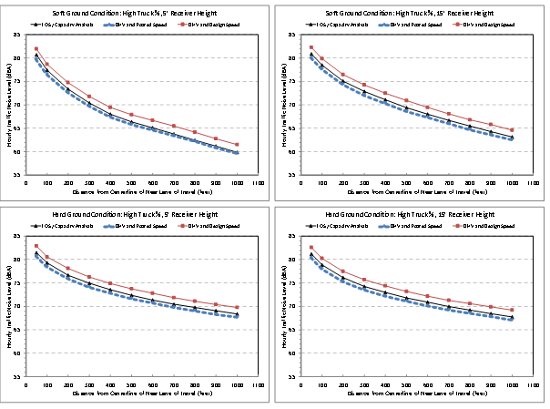
Figure I-11. TNM-calculated Noise Levels for an 8-lane Freeway using Combinations of Traffic Volumes and DHV, LOS, and Posted Speeds
One of the objectives of this study was to test the FHWA TNM's sensitivity to a non-uniform traffic distribution for a multiple-lane highway. Up to this point, the scenarios assumed a non-uniform distribution of vehicle volumes and types across multiple lanes, while maintaining a uniform speed across multiple lanes. Realizing that a uniform-speed assumption does not accurately represent real-world traffic flow on a multiple-lane highway, the study team analyzed the data collected by the Volpe Center for the Phase 1 TNM Validation Study for representative 8-lane freeways and developed the curves shown in the graph of Figure I-12.
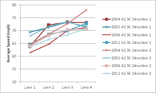
Figure I-12. Average Vehicle Speeds by Lane on Selected 8-lane Highway Facilities (based on data collected by the Volpe Center)
Each curve in Figure I-12 represents the measured average speed by lane for a particular site from the Volpe Center's dataset. As expected, the curves show slower moving vehicles on the outer lane (Lane 1) and faster moving vehicles on the inner lane (Lane 4). The study team calculated lane-average speeds and developed the speed distribution curve for an 8-lane facility with an average directional speed of 65 mph as shown in Table I-7.
The average speeds by lane in Table I-7 were combined with the non-uniform traffic (volume) distributions for the three 8-lane scenarios (at-grade, depressed, and elevated highways) described in previous sections and then compared to the corresponding reference scenario (traffic volumes and speeds evenly distributed across all lanes in each direction). The effects of modeling a non-uniform speed distribution were negligible. While TNM users may want to consider modeling non-uniform traffic (volume) distributions, there is no need to model non-uniform speed distributions. The study team recommends using the average speed for the directional traffic flow that corresponds to the modeled vehicle volume and mix (i.e., if traffic data are based on LOS volumes, use the corresponding FFS; if traffic conditions are based on DHV, use either the design speed or the posted speed).
As shown in the previous sections, the effects of a non-uniform traffic distribution for a multiple-lane highway are generally less than 1 dBA. Because other factors affecting sound propagation (e.g., rows of buildings, noise barriers, tree zones, etc.) have larger effects on calculated sound levels, traffic distributions across the lanes of multiple-lane highways may be ignored for environmental noise studies prepared in support of the permitting process under the National Environmental Protection Act (NEPA). One of the objectives of a traffic noise study performed in support of the NEPA process is to compare the extent of noise impact and preliminary noise abatement costs for multiple alternatives to the Proposed Action. The return on the investment of extra resources to develop traffic distributions across the lanes of a multiple-lane highway is negligible at the planning stage of a project. Although the effect of a non-uniform traffic distribution is small, it deserves consideration during the final design stage of a highway project, when final decisions about noise barriers will be made.
The recommended Best Practices for modeling non-uniform traffic distributions on a multiple-lane highway are summarized as follows:
As required by FHWA and all SHAs, a highway noise analysis is performed for the loudest hour of the day. The loudest hour of the day is dependent upon traffic conditions - vehicle volume, operating speed, and number of trucks - that combine to produce the highest hourly noise levels adjacent to the highway corridor. According to FHWA guidance, the “worst hourly traffic noise impact” usually occurs at a time when truck volumes and vehicle speeds are the greatest, typically when traffic is free flowing and at or near LOS C conditions. Based on this guidance, the use of traffic data that are based on LOS is the preferred approach. However, realizing that detailed traffic projections are not necessarily developed for all highway projects, this report offers the following recommended Best Practices for the use of traffic data in highway noise studies:
[1] Available at: https://www.fhwa.dot.gov/environment/noise/traffic_noise_Model/model_validation/
[2] Rochart, Judith L. and Gregg G. Fleming, "TNM Version 2.5 Addendum to Validation of FHWA's TNM® (TNM) Phase 1, Final Report,” U.S. Department of Transportation, Federal Highway Administration, FHWA-EP-02-031 Addendum and DOT-VNTSC-FHWA-02-01 Addendum, July 2004.
[3] Available at: https://www.fhwa.dot.gov/environment/noise/traffic_noise_model/tnm_faqs/
[4] Available at: http://www.nhi.fhwa.dot.gov/training/course_search.aspx?tab=0&key=142051&course_no=142051&res=1#more_information
[5] Available at: http://www.trb.org/NCHRP/Blurbs/171433.aspx
[7] Bossler, Dr. John D., Dr. David J. Cowen, James E. Geringer, Susan Carson Lambert, John J. Moeller, Thomas D. Rust, Robert T. Welch. “Report Card on the U.S. National Spatial Data Infrastructure - Compiled for the Coalition of Geospatial Organizations.” February 6, 2015.
[8] See an overview of the North Carolina Department of Transportation (NCDOT) geospatial standards and practices at https://connect.ncdot.gov/resources/gis/Pages/GIS-Standards.aspx.
[9] Sugarbaker, L.J., Constance, E.W., Heidemann, H.K., Jason, A.L., Lukas, Vicki, Saghy, D.L., and Stoker, J.M., 2014, “The 3D Elevation Program initiative-A call for action: U.S. Geological Survey Circular 1399,” 35 p., https://pubs.usgs.gov/circ/1399/.
[10] “Triangulated irregular network” on https://en.wikipedia.org/wiki/Triangulated_irregular_network.
[11] Some useful sites that provide more detailed information about elevation datasets include:
[12] See https://nationalmap.gov/about.html
[13] Users of the FHWA TNM in Massachusetts, Montana, and Tennessee identified The National Map as a source of geospatial data for highway projects.
[14] See https://nationalmap.gov/elevation.html
[15] See https://nationalmap.gov/3DEP/3dep_transition.html
[16] The National Map Viewer may be found at https://viewer.nationalmap.gov/basic/.
[17] Elevation data Quality Levels (QL) for the 3DEP initiative range from QL1 to QL5, with a QL1 designation representing the highest level of accuracy for elevation data. These data Quality Levels are in terms of four parameters. One parameter is the vertical error in elevation datasets, defined in terms of the root mean square error in the z- dimension (RMSEz), which ranges from 10 centimeters for QL1 to 185 centimeters for QL5. Another parameter is the DEM cell size, which ranges from 0.5 meters for QL1 to 5 meters for QL5. The goal of the 3DEP initiative is to achieve a data quality level of QL2 nationally by 2022. The specifications for QL2 include an RMSEz of 10 centimeters and a DEM cell size of 1 meter.
[18] See: https://www.mass.gov/learn-about-massgis
[19] A “dummy lane” is a TNM roadway without traffic. The width of the dummy lane is modeled such that the outer edge of the lane defines the diffracting edge of the roadway.
[20] See Appendix E of Report 791.
[21] Transportation Research Board, “Highway Capacity Manual,” National Research Council, Washington, D.C., 2000.
[22] See: https://ops.fhwa.dot.gov/freight/freight_analysis/nat_freight_stats/docs/13factsfigures/pdfs/fff2013_highres.pdf
[23] American Association of State Highway and Transportation Officials. (2011). A Policy on Geometric Design of Highways and Streets. Washington, D.C.
[24] The TNM 2.5 runs also included a receiver at a distance of 25 feet from the centerline of the near lane of travel. The TNM results for that receiver location are not presented in this report, because the study team felt that, in the end, the 25-foot receiver location was not representative of a “real world” scenario.

