


- Household Travel
- Trends in Our Nation's Travel
- Usual and Actual Commute: A Typical Day Versus a Specific Day
- Baby Boomer Travel Trends
- Travel of Millennials
- Aging of the Household Vehicle Fleet
- Some Myths and Facts About Daily Travel
- Myth 1: The majority of personal travel is for commuting to work
- Myth 2: Americans love their cars, and that's why they don't walk or take transit
- Myth 3: Households without vehicles rely completely on transit, walk, and bike
- Myth 4: When elderly drivers give up their driver's license they maintain mobility by using transit or walking instead of using private vehicles
- Myth 5: We can solve congestion by having people shift noncommuting trips outside of peak periods
- Gas Prices and the Public's Opinions
- Freight Movement
Household Travel
To fully understand daily travel, one must look at it through the lens of the 300 million Americans who are using the transportation system to connect to their jobs, markets, educational facilities, healthcare services, airports, recreational places, and more. The National Household Travel Survey (NHTS) is unique in that it is the only national source of travel data that connects the characteristics of the trip (e.g., mode used, trip purpose, distance) with the characteristics of the household (e.g., income, vehicle ownership, location) and of the individual making the trip (e.g., age, sex, education, worker status). As such, it allows for observation of daily travel behavior and fluctuations in that behavior through the lens of socio-demographic and economic changes in the country. The 2009 NHTS, the most recent survey, was sponsored primarily by the Federal Highway Administration (FHWA), with participation by the Federal Transit Administration (FTA), the American Association of Retired Persons (AARP), and American Automobile Association. The FHWA Office of Highway Policy and Information serves as the project manager for the survey.
It is crucial to understand travel behavior in the context of demographics and location. The average transportation project has a 20-year span from definition of potential need to full completion. The more the relationship between travel behavior and the demographics of the public and the location of homes and workplaces can be documented, the better future needs can be determined and resources effectively used. This chapter describes some elements of how travel is changing as the Nation is changing.
Since 1969, NHTS has collected personal travel information intermittently using a national sample of households in the civilian noninstitutionalized population. The survey captures a snapshot of the American public’s daily travel behavior. It is crucial that the information used to guide policies that impact our transportation system is based on sound statistical data, such as that from the NHTS. The 2009 NHTS data were collected from March 2008 through April 2009, which covered a period when there was a drop in vehicle miles of travel and, in some places, an increase in transit use.
|
NHTS Methodology and Timing The NHTS collects travel data from a representative sample of U.S. households to characterize personal travel patterns. The survey obtains demographic characteristics of households and people and information about all vehicles in the household. Details of travel by all modes for all purposes of each household member are collected for a single assigned travel day. In this way, NHTS traces both the interaction of household members and the use of each household vehicle throughout an average day. The data provide national and, with the 2009 survey, State-level estimates of trips and miles by travel mode, trip purpose, time of day, gender and age of traveler, and a wide range of attributes. Much of the data presented in this section are from the NHTS data series, unless otherwise noted. Since 1990, NHTS data have been collected using a random-digit dial sample of telephone households in the United States. Prior to 1990, NHTS data were collected in face-to-face interviews sampled from respondents to the Census Bureau's Current Population Survey. The 2008–2009 NHTS data were collected during a time when the price of gas was hitting a peak of $4 per gallon, unemployment was on the rise, the stock market was falling, and the housing market was declining. The survey results, particularly the decline in household-based vehicle miles traveled (VMT), should be considered against this backdrop. Note that the previous survey in the series, the 2001 NHTS, was also conducted during an economic downturn. Additional information on NHTS is available at www.fhwa.dot.gov/policyinformation/nhts.cfm or http://nhts.ornl.gov. |
This section contains a discussion of the recent decline in vehicle miles traveled (VMT), the disparity of this decline in urban versus rural areas, and how the decline differed by trip purpose. The section also contains a comparison of the usual mode of travel to work with the actual mode used, the influence of the Baby Boomers on total travel, and the aging of the household vehicle fleet. Five commonly held myths about travel are discussed, and the chapter concludes with a discussion of the public’s opinions of travel issues and the related gas price spike in the summer of 2008.
This portion of Chapter 1 presents some of the trends in travel behavior that can be gleaned from the NHTS data. The data allow for analysis of other topics and issue areas as well as tabulations at the national and local levels. As technology continues to impact communications and transportation, the need to track the intersection of demographics and travel behavior increases.
Trends in Our Nation’s Travel
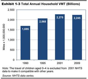
The NHTS results show a consistent increase in VMT during the three-decade period from 1969 through 2001 but a decrease in VMT between 2001 and 2009. As shown in Exhibit 1-2, the total number of trips has increased over time from 1990 through 2009, but household VMT decreased between 2001 and 2009. Americans drove 30 billion fewer vehicle miles in 2008-2009 than in the 2001-2002 NHTS survey period, as shown in Exhibit 1-3, even though the population grew by almost 10 percent during that period.
| 1990 | 1995 | 2001 | 2009 | |
|---|---|---|---|---|
| Household Vehicle Trips | 193,916 | 229,745 | 233,030 | 233,849 |
| Household VMT | 1,695,290 | 2,068,368 | 2,274,769 | 2,245,111 |
| Person Trips | 304,471 | 378,930 | 384,485 | 392,023 |
| Person Miles of Travel | 2,829,936 | 3,411,122 | 3,783,979 | 3,732,791 |
1. The travel of children aged 0-4 is excluded from 2001 NHTS data to make it comparable with other years.
2. 1990 person and vehicle trips were adjusted to account for survey collection method changes.
3. Vehicle miles and person miles are only calculated on trips with distance reported.
The NHTS results also show that transit ridership increased by 16 percent from 2001 to 2009, far outstripping the population growth during that time period. Most of the increase in transit use was for shopping and social/recreational activities other than visiting friends and relatives. This category includes going to movies, plays, restaurants, sporting events, and recreational activities like playing sports and going to the gym.
Geographic Trends in Trip Rates and Trip Lengths
Two basic factors used in land use planning and travel demand forecasting are where people live and where they work. Each time people leave their places of residence, work places, or elsewhere, they generate a “trip,” and the distance traveled and other attributes of the trip are captured in the survey.
As reflected in Exhibit 1-4, daily travel shows a steady increase from 1969 to 2001. Daily person trips peaked in 1995 at 4.30 trips per person per day. Daily miles per person showed a slightly different pattern, peaking in 2001 at 40.25 miles per person per day and declining to 36.13 miles per person per day in 2009. The average person trip length also decreased in 2009 when compared to 2001; average person trip length in 2001 was 10.04 miles and in 2009 it was 9.75 miles, which reduced the average person trip by approximately one-quarter of a mile. On the surface, one-quarter of a mile may not appear to be considered significant, but when you multiply it by more than 3 billion person trips, the results become notable.
| 1969 | 1977 | 1983 | 1990 | 1995 | 2001 | 2009 | |
|---|---|---|---|---|---|---|---|
| Per Person | |||||||
| Daily Person Trips (count) | 2.02 | 2.92 | 2.89 | 3.76 | 4.3 | 4.09 | 3.79 |
| Daily PMT (miles) | 19.51 | 25.95 | 25.05 | 34.91 | 38.67 | 40.25 | 36.13 |
| Per Driver | |||||||
| Daily Vehicle Trips (count) | 2.32 | 2.34 | 2.36 | 3.26 | 3.57 | 3.35 | 3.02 |
| Daily VMT (miles) | 20.64 | 19.49 | 18.68 | 28.49 | 32.14 | 32.73 | 28.97 |
| Per Household | |||||||
| Daily Person Trips (count) | 6.36 | 7.69 | 7.2 | 8.94 | 10.49 | 9.81 | 9.5 |
| Daily PMT (miles) | 61.55 | 68.27 | 62.47 | 83.06 | 94.41 | 96.56 | 90.42 |
| Daily Vehicle Trips (count) | 3.83 | 3.95 | 4.07 | 5.69 | 6.36 | 5.95 | 5.66 |
| Daily VMT (miles) | 34.01 | 32.97 | 32.16 | 49.76 | 57.25 | 58.05 | 54.38 |
| Per Trip | |||||||
| Average person trip length (miles) | 9.67 | 8.87 | 8.68 | 9.47 | 9.13 | 10.04 | 9.75 |
| Average vehicle trip length (miles) | 8.89 | 8.34 | 7.9 | 8.85 | 9.06 | 9.87 | 9.72 |
1. Average trip length is calculated using only those records with trip mileage information present.
2. 1990 person and vehicle trips were adjusted to account for survey collection method changes.
|
NHTS Terminology Trip Chain or Linked Trip – Individual trips or trips that are linked together to a destination. Any movement from one address to another, except if only to change mode of transport. Person Trip – Any trip made by one person regardless of mode (auto, truck, transit, walk, bike, etc.). Person Miles of Travel – The miles associated with a person trip. Vehicle Trip – Any movement of a vehicle from one address to another, regardless of the number of vehicle occupants. Vehicle Miles Traveled (VMT) – The miles associated with a vehicle’s movement, regardless of the number of occupants. |
Examining trends by geographic location can provide a better understanding of where these changes are occurring. In 2009, the data showed that there was a significant decrease in passenger trips and passenger miles in both urban and rural areas compared to 2001 (see Exhibit 1-5).
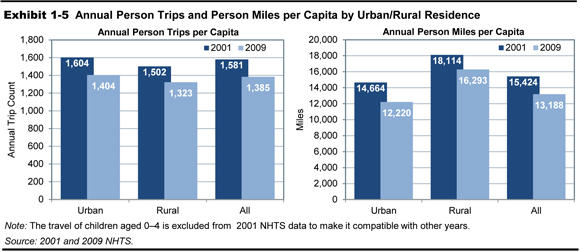
However, residents of urban areas reduced their person trips and person miles of travel more than those living in rural areas. For every decrease of one person trip in rural areas, there was a decrease of two person trips in urban areas. In addition, per capita, there was about a 14.5-percent overall decrease in person miles. In urban areas, the largest person-mile decrease happened at slightly less than 17 percent, whereas there was about a 10 percent decrease in rural areas.
Despite increases in aggregate personal VMT through 2001, a number of indicators point toward saturation in vehicle trips and vehicle miles of travel per person, with the peak of most per-person and per-household statistics occurring in 1995. Several factors could be possible explanations for this apparent saturation, such as the desire to limit the time spent in travel and replacing physical trips with electronic communication or online shopping. Given both the gas price spike in the summer of 2008 and the economic recession starting in autumn of that year, it is difficult to isolate how much of the reduction in travel was the product of these two events and how much was the product of broader changes. The proposed 2015 NHTS will add a crucial data point for continuing to track trends in travel behavior.
The Determinants of Travel
The NHTS is the only national data source that asks the American public why they took a given trip. The purpose of travel is significant because it provides a tool for anticipating travel volumes and demand given predictions of demographic change. Purposes are classified into a number of categories: to work, for work-related business, to shop, to run family or personal errands, to school or church, and to make social or recreational trips.
|
NHTS Non-Work Trip Purposes Social/recreational trips include activities such as going out for a meal; visiting friends or relatives; going to a movie or play; and exercising, playing sports, or going to the gym. Two other significant purposes of travel are (1) shopping and (2) other family and personal errands, which includes purchase of services such as haircuts or dry cleaning, picking up or dropping off someone else, or other family or personal errands and obligations. |
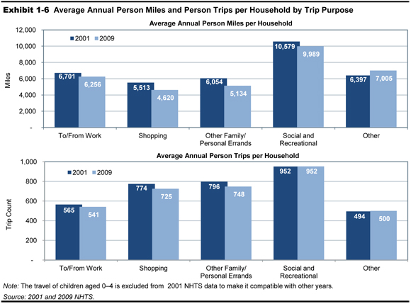
The 2009 data show that the declines in person miles and person trips were most notable in travel to and from work, personal and family errands, and social and recreational travel, while shopping and trips for other purposes were relatively constant. Travel to work shows a 10-percent decrease in miles and a 7-percent decrease in trips between 2001 and 2009. In 2009, American households were traveling 13.9 percent less for family or personal errands, and trip lengths for these family errands also dropped by 10 percent compared to 2001. In addition, daily person miles for social and recreational purposes declined by 9.5 percent between 2001 and 2009. (See Exhibit 1-6.) Two of the three purpose groupings—errands and social/recreational—are those for which most households have the greatest discretion in amount of travel. Further research of this behavior would be useful for policy considerations because family and personal errands and social and recreational travel have generally been the two most prevalent reasons for travel since 1990. This research would combine NHTS data with other sources to determine the extent to which reduction in these trips between 2001 and 2009 was due to the economic environment at the time or to structural changes in how Americans view daily travel. The latter would have impact on transportation policy and priorities.
Travel by Time of Day
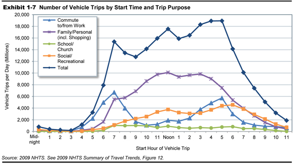
NHTS data allow for an examination of vehicle trips by purpose and time of day. Peak travel period information is salient to the study of congestion. Exhibit 1-7 shows the morning and evening peak periods by vehicle trip purpose. Predictably, the traditional peaks of 6 to 9 in the morning and 4 to 7 in the evening reflect commuting to and from work. There is an additional minor peak in total vehicle trips around noon. According to the 2009 NHTS, 34.8 percent of workers have the option of flexible arrival times and about 11 percent of workers have the option of working from home some of the time. This increased flexibility is one of the factors that appears to be reflected in the pattern of travel by time of day. Most of these vehicle trips were for family and personal errands, which are more prevalent between noon and 3 p.m.
Usual and Actual Commute: A Typical Day Versus a Specific Day
The NHTS has questions designed to capture both the “usual” mode of travel to work in a traveler’s previous work week and the “actual” mode of commuting on a specific Travel Day recorded in a travel diary. Comparing the usual mode to the actual travel day trip provides a measure in the day-to-day variability in commute modes, as well as a check on the tendency of respondents to give socially desirable responses. This comparison is particularly important because it gives context to the data on usual mode to work that is collected in the annual American Community Survey (ACS) that replaced the Decennial Census Long Form after 2000. The ACS data on commuting is widely used in State and metropolitan transportation planning, and inclusion of the NHTS comparison on usual versus actual mode helps put the ACS commute data in an appropriate context. This is important because the trip to work is central to the transportation planning process, particularly for the travel demand models used in developing metropolitan and statewide transportation plans.
The comparisons in Exhibit 1-8 between usual and actual mode of travel show that 93 percent of workers who reported that that they usually drive alone did indeed drive alone on their assigned Travel Day. On the other hand, only about 80 percent of workers who said they usually walk to work actually walked on their assigned Travel Day. Carpoolers showed the greatest change in their comparison of usual to actual travel between 2001 and 2009; in 2001, 75 percent of workers who reported they usually carpooled did carpool on their travel day, but by 2009, only about 55 percent of those who reported that they usually carpooled actually did carpool, and 43 percent of those who reported that they usually carpooled actually drove alone. Finally, for those who said they usually took transit, about 68 percent actually did take transit on Travel Day, and when these individuals did change their mode, about 13 percent of these then switched to driving alone and another 9 percent carpooled.
| Usual Commute Mode | Actual Commute Mode on Travel Day | |||||
|---|---|---|---|---|---|---|
| Drove Alone | Carpool | Transit | Walk | Bike | Other | |
| Drove Alone | 93.5 | 5.6 | 0.1 | 0.5 | 0.1 | 0.4 |
| Carpool | 42.9 | 54.8 | 0.5 | 1.0 | 0 | 0.8 |
| Transit | 13.2 | 9.2 | 68.3 | 6.6 | 0.8 | 1.9 |
| Walk | 6.1 | 9.3 | 3.4 | 80.2 | 0.2 | 0.7 |
| Bike | 13.8 | 3.3 | 6.0 | 2.6 | 73 | 1.4 |
| Other | 64.1 | 19.0 | 4.2 | 4.3 | 0.3 | 8 |
Baby Boomer Travel Trends
By 2050, about one in four members of the U.S. population will be over the age of 65. The cohort of people age 65 and older is projected to grow by another 60 percent during the next 15 years or until 2035. Maintaining the mobility of this group of people 65 or older is a major issue both for the group and for their adult children, who often bear the responsibility for transporting their parents.
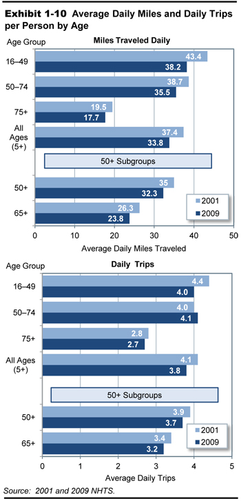
In 2009, people age 65 and older made about 45.5 billion trips, which represented an 11-percent increase in this cohort’s total travel from 2001. This total travel encompassed all modes of travel including household private vehicles, transit, motorcycles, walking, and biking. However, travel per capita for this age group declined. For this aging group, the per-person measures of trips and miles decreased by about 6 percent and 12 percent, respectively, from 2001. Exhibit 1-9 shows that, in 2009, women in this age range make 17 percent fewer daily trips and travel about one-third less than men in the same age range. The NHTS recorded 89 percent of older men as drivers, compared with only 73 percent of older women. This trend is expected to change as the percentage of women drivers age 65 or older increases. Women who turn 65 today most likely grew up driving, and, as such, the percentage of women drivers 65 and older, while historically low, will become closer to that of older men. Exhibit 1-10 shows the decrease in per capita baby boomer travel between 2001 and 2009. Note that this trend is consistent with those of other age cohorts.
| Age | Total | Men | Women | |||
|---|---|---|---|---|---|---|
| 2001 | 2009 | 2001 | 2009 | 2001 | 2009 | |
| Person Trips per Person | ||||||
| Under 16 | 3.4 | 3.2 | 3.5 | 3.2 | 3.4 | 3.2 |
| 16 to 20 | 4.1 | 3.5 | 4 | 3.3 | 4.2 | 3.7 |
| 21 to 35 | 4.3 | 3.9 | 4.2 | 3.7 | 4.5 | 4.1 |
| 36 to 65 | 4.5 | 4.2 | 4.4 | 4.1 | 4.5 | 4.3 |
| Over 65 | 3.4 | 3.2 | 3.8 | 3.5 | 3.1 | 2.9 |
| Person Miles per Person | ||||||
| Under 16 | 24.5 | 25.3 | 24.6 | 27.2 | 24.4 | 23.3 |
| 16 to 20 | 38.1 | 29.5 | 34.1 | 28.2 | 42.5 | 31 |
| 21 to 35 | 45.6 | 37.7 | 49.8 | 40.5 | 41.5 | 35 |
| 36 to 65 | 48.8 | 44 | 57.7 | 50.9 | 40.4 | 37 |
| Over 65 | 27.5 | 24 | 32.9 | 30.5 | 23.5 | 19.3 |
Additional discussion of these travel trends can be found in Chapter 1 of the 2010 C&P Report, in the section titled “Aging of U.S. Population and Impact on Travel Demand.”
Travel of Millennials
Much attention has been given to changes in the travel behavior of the Millennial generation, generally defined as those born between 1982 and 2000. Compared with previous generations, youth travel has decreased. Youth are driving less, making fewer trips, and traveling shorter distances.
According to the National Household Travel Survey (NHTS) data, there are significant differences between current youth travel and the travel of youth in previous decades. Youth passenger miles traveled (PMT) on all modes of transportation in 2009 was 80 percent of PMT in 1995 and 2001. Similarly, vehicle miles of travel (VMT) in 2009 was only 75 percent of the VMT of youth in 1995 and 2001.
There is evidence to suggest that the travel choices of youth are being influenced by the constraints of their personal income. These choices may include foregoing vehicle ownership, driving less, and taking more public transit.
In addition, current national housing trends have shown that younger populations, although less settled than older populations, prefer to live in urban areas. As young people continue to gravitate towards urban areas, they will become accustomed to living in places that offer a variety of travel options.
|
Emerging Trends in Youth Travel: What Is Happening and Why? High unemployment and personal income constraints due to the recession limit resources for travel. Youth are still living at home with parents and sharing the family vehicle. Increases in driver’s licensing restrictions have resulted in more youth waiting longer to get their licenses. Youth prefer to live in high-density areas where there are more modal options and shorter trip lengths. Technology influences travel and how youth get their information. Youth concerns for the environment play a role in their travel decisions. |
Driver’s licensing rates also show a drop between 1995 and 2009. In both 1995 and 2001, 86 percent of all 16-to-28-year-old males were licensed drivers; this drops to 80 percent in 2009. For 16-to-29-year-old females, the licensing rate stays stable at approximately 82 percent across all 3 survey years.
These are some of the emerging factors that are influencing the travel decisions of youth. Together, they warrant further discussion on emerging issues related to travel demand, transportation policy, and the needs and perspectives of those who are soon to be the most predominate users of the transportation system. These and other issues are the topic of research conducted by FHWA (Federal Highway Administration, Office of Transportation Policy Studies, The Next Generation of Travel: Final Report, 2013).
Aging of the Household Vehicle Fleet
Like the population as a whole, the household vehicle fleet is also aging. NHTS collects information about household vehicles, including make, model, model year, estimates of annual mileage, and which household member is the primary driver (see Exhibit 1-11). The basic pattern over time is a consistent decrease in household size matched with an increase in vehicles per household.
| 1969 | 1977 | 1983 | 1990 | 1995 | 2001 | 2009 | |
|---|---|---|---|---|---|---|---|
| Persons per household | 3.16 | 2.83 | 2.69 | 2.56 | 2.63 | 2.58 | 2.50 |
| Vehicles per household | 1.16 | 1.59 | 1.68 | 1.77 | 1.78 | 1.87 | 1.86 |
In 2009, there were about 211 million household vehicles or about 1.86 vehicles per household. Between 2001 and 2009, there was a 0.58-percent annual increase in the average number of household vehicles, in contrast to the long-term annual increase of 2.7 percent over the 40-year period between 1969 and 2009. This indicates that American households continue to depend heavily on automobiles, but appear to be reaching saturation in household vehicle ownership. On the other hand, the number of households with no vehicle available grew slightly by nearly 1 million households, representing a slight increase from 8.1 percent to 8.7 percent of all households. This may be due to changes in economic conditions or household location.
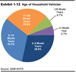
The aging of the household vehicle fleet continues to impact fuel consumption, air quality, and safety. Because over half the household vehicles on the road are more than 9 years old, recent automotive advances in energy efficiency, air quality, and safety are not fully realized in the national vehicle fleet. The 2009 NHTS reflects that the average age of a household vehicle increased from 8.87 years in 2001 to 9.38 years in 2009. In 2009, only 6 percent of household vehicles were 1 year old or newer, 32 percent of vehicles were between 2 and 5 years old, 34 percent were between 6 and 10 years old, and 7 percent were 20 years old or more (see Exhibit 1-12).
Some Myths and Facts About Daily Travel
This section explores five common misperceptions about travel and what the actual data reveal about these issues.
Myth 1: The majority of personal travel is for commuting to work.
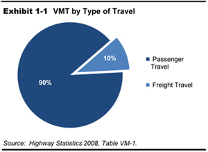
Perhaps surprisingly, travel to and from the workplace accounts for only 16 percent of all person trips and 28 percent of all vehicle miles. Only 54 percent of the total population are workers, and 76 percent of the population generally regarded as working age (age 16 to 64) are employed. Even in times of lower unemployment, this percentage does not increase significantly.
Workers drive much more than their nonworker counterparts. Workers age 16 to 64 drive an average of 11,908 miles annually for all purposes, compared to 5,592 for those of the same age who are not employed. Of those 65 and older, those with jobs drive 9,754 miles annually, compared with 4,622 annual miles for those without jobs. The variation in miles driven by employment status is striking considering that workers typically drive more than twice the miles of their nonworking counterparts. Although some of this additional driving is to commute or for work-related travel, workers drive more than nonworkers for each major trip purpose group, as shown below. Exhibit 1-13 displays trip purpose for four groups—workers 16 to 64, workers 65 or older, nonworkers 16 to 64, and nonworkers 65 or older. For workers, 35 percent of driving is for commutes to work, followed by 22 percent for social/recreational trips, and 13 percent each for family/personal errands and for shopping. Together, these four purposes account for 83 percent of driving done by workers.
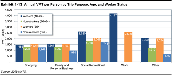
For the miles driven by the 46 percent of Americans who are not workers, social/recreational travel (34 percent of their VMT) is followed by shopping (24 percent) and family and personal business (23 percent), for a total of 81 percent of their driving.
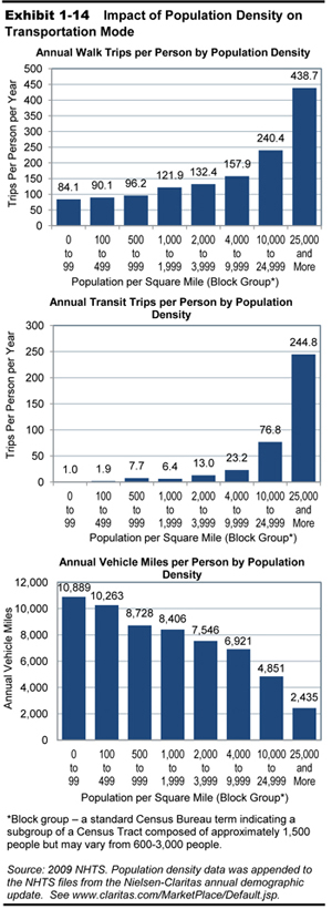
Myth 2: Americans love their cars, and that’s why they don’t walk or take transit.
Americans’ often cited “love affair” with their cars may have much more to do with the design of our neighborhoods and land use decisions than with transportation. Higher-density areas can provide more opportunities for walking, biking, and transit use than low-density areas. In some low-density neighborhoods, transit services are not cost-effective to provide and there are few destinations, such as schools, jobs, or shopping, within walking distance. People may be left with no other choice but to drive. Exhibit 1-14 visually portrays the relationship between population density and the use of transit, walking, and private vehicles.
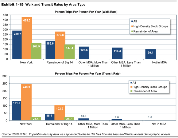
Households living in higher-density areas have more transportation choices. Of the 50 Metropolitan Statistical Areas (MSAs) with populations greater than 1 million, 14 have at least 10 percent of their populations living in high-density block groups of 10,000 or more persons per square mile. Excluding New York, which accounts for such a huge share of the Nation’s transit trip-making, residents of these 14 areas are at least 8 times more likely to make a trip on transit than those who live in MSAs of 1 million or less, and more than 50 times more likely to use transit than those living outside an MSA. Residents of a Big 14 area make walking trips at twice the rate of those in MSAs of 1 million or less, and 2.8 times more than those living outside an MSA (see Exhibit 1-15). (See the discussion of livable communities in Chapter 5 of this edition of the C&P report).
|
14 MSAs With at Least 10 Percent of People Living in High Density Block Groups of 10,000 Persons or More per Square Mile New York – 48.0% Los Angeles – 43.2% San Francisco – 33.7% Chicago – 33.0% Philadelphia – 27.7% San Diego – 26.8% Boston – 24.1% Miami – 23.1% Las Vegas – 22.2% Washington DC – 15.7% Providence – 14.4% Milwaukee – 12.2% Pittsburgh – 11.4% Sacramento – 10.4% |
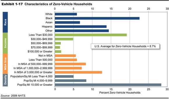
Myth 3: Households without vehicles rely completely on transit, walk, and bike.
Although zero-vehicle households rely more heavily on transit, walk, and bike modes than vehicle-owning households do, people in zero-vehicle households accomplish a majority of their travel in private vehicles owned by others. Approximately 9.8 million households, or 8.6 percent of all U.S. households, do not own a vehicle. People in zero-vehicle households average about 100 minutes of travel a day, 76 percent of which are as a driver or passenger in a private vehicle; they accomplish 50.7 percent of their person miles of travel in private vehicles.
Because the data in this section are presented as person trips and person miles, private vehicle travel includes travel in a vehicle as a driver and as a passenger. Those in zero-vehicle households could be using a car borrowed from a friend or relative or be a vehicle passenger in another household’s car. (See Exhibit 1-16.) The vehicle occupancy per private vehicle trip by members of zero-vehicle households is, as expected, consistently larger (2.06) than the occupancy rate of vehicle-owning household members (1.67).
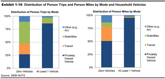
Whether the household is without a vehicle by necessity or by choice, its daily travel is considerably lower than that of vehicle-owning households. While a zero-vehicle household has half the daily person trip rate of a vehicle-owning household, their daily person miles of travel is one-fifth that of their vehicle-owning counterparts.
|
Car Share Services Some of households that are non-vehicle owning by choice are using the expanding option of car-share services, such as Zip Cars and Car2go. Unlike traditional car rental agencies, car-sharing is set up to allow rentals by the minute or the hour. These services are designed for high-density areas and often have reserved parking spaces, an especially convenient benefit for urban dwellers. The NHTS did not collect data on car-sharing in the 2009 survey, but may do so in 2015. |
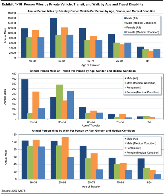
Myth 4: When elderly drivers give up their driver’s license they maintain mobility by using transit or walking instead of using private vehicles.
Like the rest of the U.S. population, the elderly are heavily dependent on private vehicle travel to meet their needs. Although some relocate, a large portion of the elderly age in place in the homes where they raised their families. Issues of diminished eyesight, response time, and physical mobility that might keep an older person from driving may also keep them from being able to walk or take transit, making them more likely to travel as a private vehicle passenger or simply stay at home.
The NHTS collects data on whether or not respondents have medical conditions that make it difficult for them to travel outside the home. As shown in Exhibit 1-18, those with a travel disability have a lower rate of transit use and walking than others of the same age and there is a slight increase in the relative use of private vehicles, particularly by older women.
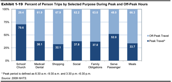
Myth 5: We can solve congestion by having people shift noncommuting trips outside of peak periods.
Encouraging the traveling public to make noncommuting trips outside of peak periods would appear to be a reasonable proposal for addressing congestion, but there are many scenarios that simply do not allow for such time flexibility. For example, picking up your child from an athletic practice or an after-school event typically needs to be done when the child is ready, not some arbitrary time after peak period. A doctor’s office would usually be open in morning and afternoon peak periods, but it would not likely be open in the evening. Although trips and travel for shopping and errand-running are not as constrained by time of day as some of the other trip purposes, many people choose to make these trips on their way to or from work.
While time-shifting may be possible for some share of trips, it is clear that the public is willing to put up with the inconvenience of congestion during peak periods to accomplish many of their travel needs. Exhibit 1-19 identifies the share of person trips in the peak period for different types of non-commuting trips.
Gas Prices and the Public’s Opinions
The price of gas rose to a nationwide average of over $3.50 per gallon in May of 2008 and did not drop below that level until October of that year. It peaked at $4.11 per gallon in June and July.
In comparing the two survey years, 2001 and 2009, average daily vehicle miles by month remained around the same through August across the 2 years possibly because the public has come to expect some increases in gas cost during the summer travel season. (See Exhibit 1-20.) In August of 2001, gas prices declined and more daily driving occurred. This follows a typical pattern of personal VMT peaking in August. However, this pattern did not repeat itself in 2008, when gas prices remained high for about 4 months and people adjusted their average daily miles. The average daily VMT per driver decreased by 13 percent in August of 2008, when gas prices remained higher than $3.80 per gallon. This apparent delayed response to high gas prices may have been because the public was waiting to see how long the phenomenon would continue. According to the NHTS data, it appears that most people decided to cut their driving in August of 2008 by an average of 3 to 4 daily miles relative to August 2001.
| Avg. Gas Price (in 2008 $) | Daily VMT per Person | Avg. Gas Price (in 2008 $) | Daily VMT per Person | |
|---|---|---|---|---|
| 2001 | 2008 | |||
| March | $1.77 | 16.6 | $3.29 | 20.4 |
| April | $1.94 | 22.3 | $3.51 | 23.1 |
| May | $2.12 | 22.7 | $3.82 | 22.2 |
| June | $2.02 | 23.4 | $4.11 | 22.0 |
| July | $1.79 | 22.9 | $4.11 | 22.6 |
| August | $1.78 | 24.0 | $3.83 | 20.8 |
| September | $1.90 | 21.8 | $3.76 | 21.2 |
| October | $1.66 | 21.9 | $3.11 | 22.8 |
| November | $1.48 | 22.3 | $2.21 | 21.6 |
| December | $1.37 | 21.3 | $1.75 | 21.1 |
| 2002 | 2009 | |||
| January | $1.40 | 21.0 | $1.84 | 19.9 |
| February | $1.41 | 23.7 | $1.98 | 22.2 |
| March | $1.57 | 22.7 | $2.01 | 22.0 |
| April | $1.76 | 21.6 | $2.10 | 21.7 |
Number One Issue for the Public: Price of Travel
Questions to elicit the public’s opinions about transportation were included in the 2009 NHTS because understanding their attitudes and perceptions is valuable when prioritizing policy. Respondents were asked to select what they considered the most important issue from a list of six pre-identified issues:
- Highway congestion
- Access to and availability of public transit
- Lack of walkways and sidewalks
- Price of travel including things like transit fees, tolls and the cost of gasoline
- Aggressive and distracted drivers
- Safety concerns.
One-third of all respondents selected the price of travel as the most important issue. When drivers were divided by demographic categories such as gender, race, income, and education, the data revealed no significant difference in their selection of travel price as the primary issue. A disproportionate share of respondents say that price of travel was their number one concern. This may have been due to the rising cost of gasoline or because of the economic recession during the data collection period.
Households with incomes of $40,000 to $70,000 ranked price as most important issue about 5 percent more often than households in both higher and lower income categories. During the post-peak period between October 2008 and April 2009, almost all households at all levels started shifting their opinions to the issues of safety and aggressive drivers (approximately 20 percent each) but 27 percent kept price as their major issue. Only households in the highest income bracket (those with incomes of $100,000 or more) selected congestion as their most important concern in this post-peak period (about 26 percent). This suggests that the gas price fluctuation remained important with middle income households throughout the study more so than with other households.
Freight Movement
The economy of the United States depends on freight transportation to link businesses with suppliers and markets throughout the Nation and the world. Freight impacts nearly every American business and household in some way. American farms and mines rely on affordable and reliable transportation to compete against their counterparts around the world. Domestic manufacturers rely on remote sources of raw materials to produce goods. Wholesalers and retailers depend on fast and reliable transportation to obtain inexpensive or specialized goods. In the expanding world of e-commerce, households and small businesses increasingly depend on freight transportation to deliver purchases directly to them. Service providers, public utilities, construction companies, and government agencies rely on freight transportation to obtain needed equipment and supplies from distant sources.
The U.S. economy requires effective freight transportation that operates at minimum cost and allows shippers and freight carriers to quickly respond to the demands for goods. As the economy grows over the next several decades, the demand for goods and the volume of freight transportation activity will only increase. Current volumes of freight are straining the capacity of the transportation system to deliver goods quickly, reliably, and cheaply. Anticipated growth of freight could overwhelm the system’s ability to meet the needs of the American economy unless public agencies and private industry work together to improve the system’s performance.
Freight Transportation System
The FHWA’s Freight Facts and Figures 2011 publication shows that the U.S. freight transportation system moves nearly 52 million tons of freight worth more than $46 billion each day to meet the logistical needs of the Nation’s 117 million households, 7.4 million business establishments, and 89,500 government units. This system includes nearly 11 million single-unit and combination trucks, nearly 1.4 million locomotives and rail cars, and more than 40,000 marine vessels. The system operates on more than 450,000 miles of arterial highways, nearly 140,000 miles of railroads, 11,000 miles of inland waterways and the Great Lakes-St. Lawrence Seaway system, and 1.7 million miles of petroleum and natural gas pipelines. The U.S. Army Corps of Engineers’ Waterborne Commerce of the United States 2007 publication identifies 146 ports that handle more than 1 million tons of freight per year.
The freight transportation system is more than equipment and facilities. As reported in Freight Facts and Figures 2011, freight transportation establishments with payrolls primarily serving for-hire transportation and warehousing employ nearly 4.2 million workers. Truck transportation businesses make up the largest freight transportation employment sector in the U.S., employing more than 2.6 million workers in 2010. Other freight transportation occupations included rail and water vehicle operators, as well as other occupations such as warehousing and storage, equipment manufacturing, equipment maintenance, and other transportation support service providers.
Freight Transportation Demand
Freight movements in the United States take a variety of forms, from the shipment of farm products across town to the shipment of electronic devices across the world. These goods move within, to, and from the U.S. via the Nation’s highways, railroads, waterways, airplanes, and pipelines, sometimes using a combination of modes to complete the trip. Due to the country’s well-developed highway network and the transport connectivity and flexibility that this network provides, the majority of freight moved within, to, or from the United States is transported by truck. Exhibit 1-21 shows a breakdown of freight movements by mode, measured by both tonnage and value of shipment.
| Mode | Tons (Millions) | Percent | Value (Billions of Dollars) | Percent |
|---|---|---|---|---|
| Truck | 12,778 | 67.7% | 10,780 | 64.7% |
| Rail | 1,900 | 10.1% | 512 | 3.1% |
| Water | 941 | 5.0% | 339 | 2.0% |
| Air, Air & Truck | 13 | <0.1% | 1,077 | 6.5% |
| Multiple Modes & Mail | 1,424 | 7.5% | 2,879 | 17.3% |
| Pipeline | 1,507 | 8.0% | 723 | 4.3% |
| Other & Unknown | 316 | 1.7% | 341 | 2.0% |
| Total | 18,879 | 100% | 16,651 | 100% |
Exhibit 1-22 shows a map illustrating the distribution of the tonnage information shown in the table in Exhibit 1-21 for truck, rail, and inland water shipments on the United States freight transportation network.
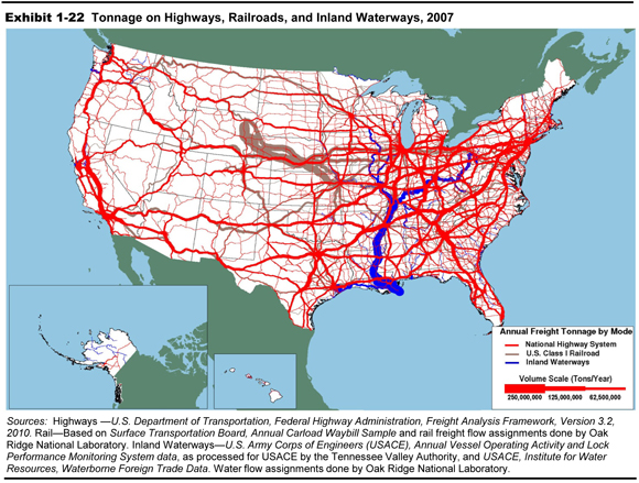
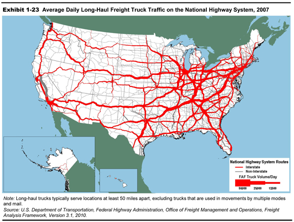
Exhibit 1-23 shows the same information as Exhibit 1-22, but only includes long-haul truck shipments on the National Highway System.
|
Freight Statistics Many of the freight statistics in this section are derived from the Freight Analysis Framework (FAF) version 3 (FAF3) and FAF version 2 (FAF2). Both versions of the FAF include all freight flows to, from, and within the United States. FAF estimates are recalibrated every 5 years, primarily with data from the Commodity Flow Survey (CFS), and are updated annually with provisional estimates. The CFS, conducted every 5 years by the Census Bureau and U.S. DOT’s Bureau of Transportation Statistics, measures approximately two-thirds of the tonnage covered by the FAF. FAF3 incorporates data from the 2007 CFS; FAF2 was based on 2002 data. Statistics on trucking activity are primarily from FHWA’s Highway Performance Monitoring System and the Census Bureau’s Vehicle Inventory and Use Survey (VIUS). The VIUS links truck size and weight, miles traveled, energy consumed, economic activity served, commodities carried, and other characteristics of significant public interest, but was discontinued after 2002. For more information, see www.ops.fhwa.dot.gov/freight/freight_analysis/faf. |
Freight movements are expected to increase over the next few decades as both the U.S. and global population grow and national and global consumer spending power increases, helping to increase demand for many types of goods. All freight transportation modes are expected to experience increased volumes, although the amount of expected growth will vary from mode to mode, as shown in Exhibit 1-24.
| Mode | 2007 | 2010 | 2040 Projected |
Compound Annual Growth, 2010–2040 |
|---|---|---|---|---|
| Truck | 12,778 | 12,490 | 18,503 | 1.3% |
| Rail | 1,900 | 1,776 | 2,353 | 0.9% |
| Water | 941 | 860 | 1,263 | 1.3% |
| Air, Air & Truck | 13 | 12 | 43 | 4.4% |
| Multiple Modes & Mail* | 1,424 | 1,380 | 2,991 | 2.6% |
| Pipeline | 1,507 | 1,494 | 1,818 | 0.7% |
| Other & Unknown | 316 | 302 | 514 | 1.8% |
| Total | 18,879 | 18,313 | 27,484 | 1.4% |
Even though the annual volume increases are modest for all modes, the cumulative 30-year growth for each mode is significant, and the increased volume will create additional strain on the entire freight transportation network, most notably the highway network. Exhibit 1-25 shows a map containing the 2040 truck tonnage information shown in Exhibit 1-24 plotted to the National Highway System.
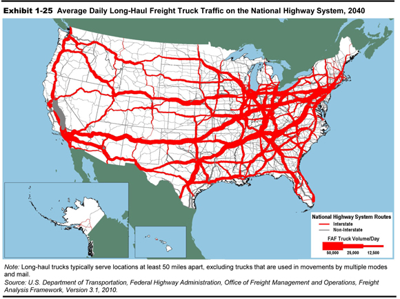
Many key truck routes on the National Highway System are expected to experience significant increases in truck volume between 2007 and 2040. These projected traffic increases would have major implications for highway congestion and freight movement efficiency, especially near large urban areas along or near major truck corridors.
The differing volume and growth characteristics of the various freight transportation modes is related in large part to each mode’s operating characteristics. These characteristics play a major role in determining how certain types of goods are transported. The routes, facilities, volumes, and service demands differ between higher-value, time-sensitive goods moving at high velocities and lower-value, cost-sensitive goods moving in bulk shipments, as shown in Exhibit 1-26.
| Parameter | Commodity Type | |
|---|---|---|
| Value Based | Tonnage Based | |
| Top Three Commodity Classes | Machinery | Gravel |
| Top Three Commodity Classes | Electronics | Cereal Grains |
| Top Three Commodity Classes | Motorized Vehicles | Coal |
| Share of Total Tons | 13% | 85% |
| Share of Total Value | 65% | 30% |
| Key Performance Variables | Reliability | Reliability |
| Key Performance Variables | Speed | Cost |
| Key Performance Variables | Flexibility | |
| Share of Tons by Domestic Mode | 87% Truck | 71% Truck |
| Share of Tons by Domestic Mode | 5% Multiple Modes and Mail | 12% Rail |
| Share of Tons by Domestic Mode | 4% Rail | 9% Pipeline |
| Share of Tons by Domestic Mode | 4% Multiple Modes and Mail | |
| Share of Tons by Domestic Mode | 3% Water | |
| Share of Value by Domestic Mode | 70% Truck | 71% Truck |
| Share of Value by Domestic Mode | 16% Multiple Modes and Mail | 12% Pipeline |
| Share of Value by Domestic Mode | 10% Air | 7% Multiple Modes and Mail |
| Share of Value by Domestic Mode | 2% Rail | 6% Rail |
| Share of Value by Domestic Mode | 2% Water | |
Though trucking typically is considered a faster mode and handles a very high volume of high-value, time-sensitive goods, it also handles a significant share of lower-value bulk tonnage. This share includes movement of agricultural products from farms, local distribution of gasoline, and pickup of municipal solid waste. The haul length is typically very short and is intraregional in nature.
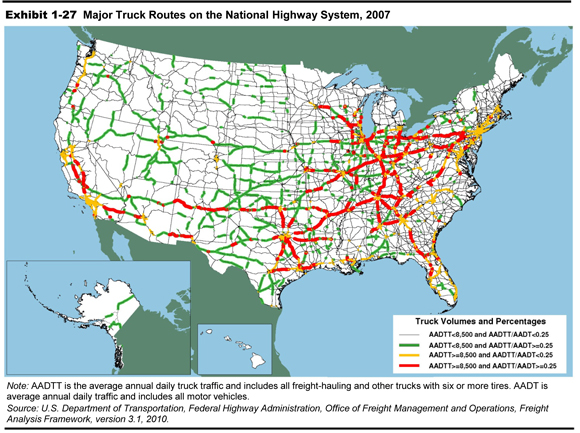
Truck movements are a significant component of overall highway traffic. Three-fourths of VMT by trucks larger than pickups and vans involves carrying freight, which encompasses a wide variety of products ranging from electronics to sand and gravel. Much of the rest of the large truck VMT is comprised of empty backhauls of truck trailers or shipping containers. Single-unit and combination trucks accounted for every fourth vehicle on almost 28,000 miles of the NHS in 2007, and 6,000 of those miles carried more than 8,500 trucks on an average day. The map shown in Exhibit 1-27 identifies those major truck routes on the National Highway System, showing the routes that handle over 8,500 trucks per day and/or experience daily traffic that is composed of at least 25 percent truck traffic.
| Location | Trucks (percent) | Truck Miles (percent) |
|---|---|---|
| Off the road | 3.3% | 1.6% |
| 50 miles or less | 53.3% | 29.3% |
| 51 to 100 miles | 12.4% | 13.2% |
| 101 to 200 miles | 4.4% | 8.1% |
| 201 to 500 miles | 4.2% | 12.1% |
| 501 miles or more | 5.3% | 18.4% |
| Not reported | 13.0% | 17.3% |
| Not applicable | 4.1% | 0.1% |
| Total | 100% | 100% |
Though many freight movements comprise long-distance shipments to domestic or international locations, a larger percentage of shipments, particularly those shipped by truck, are transported shorter distances. Approximately half of all trucks larger than pickups and vans operate locally—within 50 miles of home—and these short-haul trucks account for about 30 percent of truck VMT. By contrast, only 10 percent of trucks larger than pickups and vans operate more than 200 miles away from home, but these trucks account for more than 30 percent of truck VMT. Long-distance truck travel also accounts for nearly all freight ton miles and a large share of truck VMT. More information is shown in Exhibit 1-28.
|
Freight Data Reporting and Ton-Miles Passenger transportation volumes often use passenger-miles to measure transportation volume. The analogous measure for freight would seem to be ton-miles. Computing freight ton-miles by transportation mode is both difficult and potentially misleading for three reasons: (1) a “ton” of freight varies widely in both the nature and composition of commodities because, unlike passenger miles where a passenger is a fixed unit, for freight a ton of coal is a very different commodity than a ton of frozen ice cream; (2) freight value and tonnage often, though not always, move in opposite directions because lighter-weight goods often have higher value on a per-weight basis and are underrepresented in ton-miles measures while heavier-weight goods often are lower value on a per-weight basis and are overrepresented in ton-miles measures; and (3) ton-miles masks commodity attributes such as value and distance bracket (see Exhibit 1-28), which are important determinants of mode choice. Although computationally difficult, the Bureau of Transportation Statistics (BTS) has conducted a special tabulation of annual freight ton-miles (1980–2009) for all freight transportation modes (air, truck, railroad, domestic water transportation, and pipeline). Exhibit 1-29 represents an excerpt from the BTS tabulation and shows that railroad moves make up the largest single mode share with over 35 percent of the ton-miles, since the railroads tend to move heavy commodities over long distances. When considered in isolation the downward shift in truck ton-miles from 2005 to 2009 hides the trend of increasing truck VMT during that same time period.
Source: Bureau of Transportation Statistics, National Transportation Statistics, Table 1-50. (http://www.rita.dot.gov/bts/sites/rita.dot.gov.bts/files/publications/national_transportation_statistics/html/table_01_50.cfml).
|
|
Freight Transportation and the Cost of Goods Geographic accessibility of the major freight corridors and the performance of these corridors stimulate economic activity and create jobs. While deregulation and other factors lowered the cost of freight transportation for a given level of service over the past four decades, congestion, rising fuel prices, environmental constraints1, and other factors could increase the cost of moving all goods in the years ahead. If these factors are not mitigated, the increased cost of moving freight will be felt throughout the economy, affecting businesses and households alike. The long and often vulnerable supply chains of high-value, time-sensitive commodities are particularly susceptible to congestion. Congestion results in enormous costs to shippers, carriers, and the economy. For example, Nike spends an additional $4 million per week to carry an extra 7 to 14 days of inventory to compensate for shipping delays.2 One day of delay requires APL's eastbound trans-Pacific services to use an additional 1,300 containers and chassis, which adds $4 million in costs per year.3 A week-long disruption to container movements through the Ports of Los Angeles and Long Beach could cost the national economy between $65 million and $150 million per day.4 Freight bottlenecks on highways throughout the United States cause more than 243 million hours of delay to truckers annually.5 At a delay cost of $26.70 per hour, the conservative value used by the FHWA's Highway Economic Requirements System model for estimating national highway costs and benefits, these bottlenecks cost truckers about $6.5 billion per year. Congestion costs are compounded by continuing increases in operating costs per mile and per hour. The cost of highway diesel fuel more than doubled in constant dollars over the decade ending in 2011 and would have quadrupled if the prices at the peak in 2008 had continued.6 Future labor costs are projected to increase at a faster rate than in the past in response to the growing shortage of truck drivers.7 To attract and retain more drivers, carriers will reduce the number of hours drivers are on the road, which will in turn increase operating costs. Railroads also are facing labor recruitment challenges.8 Beyond fuel and labor, truck operating costs are affected by needed repairs to damaged equipment caused by deteriorating roads; taxes and tolls to pay for repair of infrastructure; and insurance and additional equipment required to meet security, safety, and environmental requirements. Increased costs to carriers are reflected eventually in increased prices paid for freight transportation. Between 2003 and 2009, prices increased 17 percent for truck transportation, 36 percent for rail transportation, 16 percent for scheduled air freight, 16 percent for water transportation, 41 percent for pipeline transportation of crude petroleum, 29 percent for other pipeline transportation, and 9 percent for freight transportation support activities.9 The importance of freight transportation varies by economic sector. For example, $1 of final demand for agricultural products requires 14.2 cents in transportation services, compared with 9.1 cents for manufactured goods and about 8 cents for mining products.10 An increase in transportation cost affects inexpensive (on a per-ton basis), cost-sensitive bulk commodities more than high-value, time-sensitive commodities that have higher margins. In either case, an increase in transportation costs will ripple through all these industries, affecting not only the cost of goods from all economic sectors but also markets for the goods. 1“Environmental constraints” is primarily meant to include environmental regulations that require the use of cleaner, lower emissions fuels and/or place higher taxes on higher emissions fuels.2John Isbell, “Maritime and Infrastructure Impact on Nike’s Inbound Delivery Supply Chain,” TRB Freight Roundtable, October 24, 2006 www.trb.org/conferences/FDM/Isbell.pdf. 3John Bowe, “The High Cost of Congestion,” TRB Freight Roundtable, October 24, 2006 www.trb.org/conferences/FDM/Bowe.pdf. 4U.S. Congressional Budget Office, The Economic Costs of Disruptions in Container Shipments, March 26, 2006 www.cbo.gov/ftpdocs/71xx/doc7106/03-29-Container_Shipments.pdf. 5FHWA, An Initial Assessment of Freight Bottlenecks on Highways, October 2005 www.fhwa.dot.gov/policy/otps/bottlenecks. 6FHWA, Freight Facts and Figures 2011, figure 4-2, page 50. 7Inbound Logistics. “Trucking Perspectives, 2013,” September 2013 http://www.inboundlogistics.com/cms/article/trucking-perspectives-2013/ 8Federal Railroad Administration, An Examination of Employee Recruitment and Retention in the U.S. Railroad Industry, 2007 www.fra.dot.gov/us/content/1891. 9FHWA, Freight Facts and Figures 2011, table 4-6, page 49. 10DOT, Bureau of Transportation Statistics, “The Economic Importance of Transportation Services: Highlights of the Transportation Satellite Accounts,” BTS/98-TS4R, April 1998, figure 2, page 5. |
Freight Challenges
The challenges of moving the Nation’s freight cheaply and reliably on an increasingly constrained infrastructure without affecting safety and degrading the environment are substantial, and traditional strategies to support passenger travel may not provide adequate solutions. The freight transportation challenge differs from that of urban commuting and other passenger travel in several ways:
- Freight often moves long distances through localities and responds to distant economic demands, while the majority of passenger travel occurs between local origins and destinations. Freight movement often creates local problems without local benefits.
- Freight movements fluctuate more quickly and in greater relative amounts than passenger travel. Both passenger travel and freight respond to long-term demographic change, but freight responds more quickly than passenger travel to short-term economic fluctuations. Fluctuations can be national or local. The addition or loss of just one major business can dramatically change the level of freight activity in a locality.
- Freight movement is heterogeneous compared with passenger travel. Patterns of passenger travel tend to be very similar across metropolitan areas and among large economic and social strata. The freight transportation demands of farms, steel mills, and clothing boutiques differ radically from one another. Solutions aimed at average conditions are less likely to work because the freight demands of economic sectors vary widely.
- Improvements targeted at freight demand are needed because freight accounts for a larger share of VMT on the transportation system and improvements targeted at general traffic or passenger travel are less likely to aid the flow of freight except as an incidental by-product.
Local public action is difficult to marshal because freight traffic and the benefits of serving that traffic rarely stay within a single political jurisdiction. One-half of the weight and two-thirds of the value of all freight movements cross a State or international boundary. Federal legislation established metropolitan planning organizations (MPOs) in the 1960s to coordinate transportation planning and investment across State and local lines within urban areas, but freight corridors extend well beyond even the largest metropolitan regions and usually involve several States. Various provisions in MAP-21, most notably the requirement to develop a National Freight Strategic Plan outlined in Section 1115, discuss the need to develop a process to address multi-State projects and encouraging jurisdictions to collaborate with one another to address freight transportation needs. MAP-21 Section 1118, which discusses the development of State freight plans, can assist States and other organizations working with the States to identify freight transportation needs both within the State and also at the States’ borders. Creative and ad hoc arrangements are often required through pooled-fund studies and multi-State coalitions to plan and invest in freight corridors that span regions and even the continent, but there are few institutional arrangements that coordinate this activity. One example of a more established multi-State arrangement is the I-95 Corridor Coalition. Additional information about this coalition and similar groups can be found at www.ops.fhwa.dot.gov/freight/corridor_coal.htm.
The growing needs of freight transportation can bring into focus conflicts between interstate and local interests. Many communities do not want the noise and other aspects of trucks and trains that pass through with little benefit to the locality, but those transits can have a huge impact on national freight movement and regional economies.
|
Challenges for Freight Transportation: Congestion Congestion affects economic productivity in several ways, including requiring higher but less-productive labor levels, higher inventory levels, increased equipment use, and a larger number of distribution centers serving smaller geographic areas. Workers’ commuting time also increases when congestion increases. The growth in freight is a major contributor to congestion in urban areas and on intercity routes, and congestion affects the timeliness and reliability of freight transportation. Growing freight demand increases recurring congestion at freight bottlenecks, places where freight and passenger service conflict with one another, and where there is not enough room for local pickup and delivery. Congested freight hubs include international gateways such as ports, airports, and border crossings, and major domestic terminals and transfer points such as Chicago’s rail yards. Bottlenecks between freight hubs are caused by converging traffic at highway intersections and railroad junctions, steep grades on highways and rail lines, lane reductions on highways and single-track portions of railroads, and locks and constrained channels on waterways. A preliminary study for the FHWA identified intersections in large cities, where both personal vehicles and trucks clog the road, as the largest highway freight bottlenecks.1 As passenger cars and trucks compete for space on the highway system, commuter and intercity passenger trains compete with freight trains for space on the railroad network. Rail freight is growing at the same time that rising fuel prices and environmental concerns are encouraging greater use of commuter and intercity rail. Congestion also is caused by restrictions on freight movement, such as the lack of space for trucks in dense urban areas and limited delivery and pickup times at ports, terminals, and shipper loading docks. One estimate of urban congestion attributes 947,000 hours of vehicle delay to delivery trucks parked at curbside in dense urban areas where office buildings and stores lack off-street loading facilities.2 Limitations on delivery times place significant demands on highway rest areas when large numbers of trucks park outside major metropolitan areas waiting for their destination to open and accept their shipments.3 Bottlenecks cause recurring, predictable congestion in various, high transportation volume locations. Additionally, less predictable, non-recurring congestion can also create challenges for freight movements, especially those that are time-sensitive. Sources of nonrecurring delay include traffic incidents, weather, work zones, and other disruptions. These nonrecurring, often-unpredictable, sources of highway delay have been estimated to exceed delay from recurring congestion.4 Weather, maintenance activities, and incidents have similar effects on aviation, railroads, pipelines, and waterways. Aviation is regularly disrupted by local weather delays; and inland waterways are closed by regional flooding, droughts, and ice. Chapter 5 includes a broader discussion of system performance, including congestion’s impacts on system performance. 1FHWA, An Initial Assessment of Freight Bottlenecks on Highways, October 2005 www.fhwa.dot.gov/policy/otps/bottlenecks.2Oak Ridge National Laboratory, Temporary Losses of Highway Capacity and Impacts on Performance: Phase 2, 2004, table 36, page 88 www-cta.ornl.gov/cta/Publications/Reports/ORNL_TM_2004_209.pdf. 3FHWA, Study of Adequacy of Commercial Truck Parking Facilities, 2002 https://www.fhwa.dot.gov/publications/research/safety/01158/index.cfm. 4Oak Ridge National Laboratory, Temporary Losses of Highway Capacity and Impacts on Performance: Phase 2, 2004, table 41, page 101 www-cta.ornl.gov/cta/Publications/Reports/ORNL_TM_2004_209.pdf. |
|
Challenges for Freight Transportation: Safety, Energy, and the Environment Freight transportation is not just an issue of product throughput and congestion. The growth in freight movement has heightened public concerns about safety, energy consumption, and the environment. Highways and railroads account for nearly all fatalities and injuries involving freight transportation. Most of these fatalities involve people who are not part of the freight transportation industry, such as trespassers at railroad facilities and occupants of other vehicles killed in crashes involving large trucks. The FHWA’s Freight Facts and Figures 2011 publication shows that, of the 33,808 highway fatalities in 2009, 1.5 percent were occupants of large trucks and 7.5 percent were others killed in crashes involving large trucks (the remaining 91 percent of fatalities were attributed to other types of personal and commercial vehicles). Chapter 5 of Freight Facts and Figures 2011 discusses highway safety in more detail. According to Freight Facts and Figures 2011, single-unit and combination trucks accounted for 26 percent of all gasoline, diesel, and other fuels consumed by motor vehicles, and 74 percent of the fuel consumed by freight transportation in 2009. Fuel consumption by trucks resulted in 78 percent of the 365.6 million metric tons of carbon dioxide (CO2) equivalent generated by freight transportation, and freight accounted for 26 percent of transportation’s contribution to this major greenhouse gas. Trucks and other heavy vehicles that operate on the U.S. highway system also are a major contributor to air-quality problems related to nitrogen oxide (NOx) (33 percent of all mobile sources) and particulate matter of 10 microns in diameter or smaller (PM-10) (23.3 percent of all mobile sources). Freight modes combined account for 49 percent of all mobile sources of NOx and 36 percent of all mobile sources of PM-10. Environmental issues involving freight transportation go well beyond emissions. Disposal of dredge spoil, the mud and silt that must be removed to deepen water channels for commercial vessels, is a major challenge for allowing larger ships to berth. Land-use and water-quality concerns are raised against all types of freight facilities, and invasive species can spread through freight movement. Incidents involving hazardous materials exacerbate public concern and cause real disruption. Freight Facts and Figures 2011 shows that, of the 14,783 accident-related hazardous materials transportation incidents in 2010, highways accounted for 12,635 accidents, air accounted for 1,293 accidents, rail accounted for 750 accidents, and water accounted for 105 accidents. The railcar fire in the Howard Street tunnel under Baltimore City in 2001 illustrates the perceived and real problems of transporting hazardous materials. This incident, which occurred on tracks next to a major league baseball stadium at game time during the evening rush hour, forced the evacuation of thousands of people and closed businesses in much of downtown Baltimore. A vital railroad link between the Northeast and the South, as well as a local rail transit line and all east-west arterial streets through downtown, were closed for an extended period. |
Beyond the challenges of intergovernmental coordination, freight transportation raises additional issues involving the relationships between public and private sectors. Virtually all carriers and many freight facilities are privately owned. Freight Facts and Figures 2011 shows that the private sector owns $1.001 trillion in transportation equipment plus $656 billion in transportation structures. In comparison, public agencies own $592 billion in transportation equipment plus $2.94 trillion in highways. Freight railroad facilities and services are owned almost entirely by the private sector, while trucks owned by the private sector operate over public highways. Likewise, air cargo services owned by the private sector operate in public airways and mostly at public airports. Privately owned ships operate over public waterways and at both public and private port facilities. Most pipelines are privately owned but significantly controlled by public regulation. In the public sector, virtually all truck routes are owned by State or local governments, and airports and harbors are typically owned by regional or local authorities. Air and water navigation is typically handled at the Federal level, and safety is regulated by all levels of government. As a consequence of this mixed ownership and management, most solutions to freight problems require joint action by both public and private sectors. Financial, planning, and other institutional mechanisms for developing and implementing joint efforts have been limited, inhibiting effective measures to improve the performance and minimize the public costs of the freight transportation system. In an effort to address these challenges, MAP-21 Section 1117 encourages the creation of State freight advisory committees composed of public and private sector freight stakeholders to help States identify key freight transportation needs within their jurisdictions and across State boundaries. Likewise, MPOs can form their own freight advisory committees to engage public and private sector freight professionals to identify and address freight transportation needs within their metropolitan areas.
|
National Freight Policy The recent passage of the Moving Ahead for Progress in the 21st Century (MAP-21) transportation reauthorization created a formal U.S. policy to improve the condition and performance of the national freight network to ensure that it allows the United States to compete in the global economy and achieve various goals that will improve freight movement in the U.S. (Section 1115). This policy greatly increases the visibility and emphasis on freight transportation at the federal level. MAP-21 requires the designation of a primary freight network, the creation of a critical rural freight corridors designation, the creation of a national freight strategic plan, the creation of a freight conditions and performance report, and the creation of new or refinement of existing transportation investment and planning tools to evaluate freight-related and nonfreight-related projects. All of these provisions, as well as other related provisions in MAP-21—such as prioritizing of projects to improve freight movement (Section 1116)—encouraging States to establish freight advisory committees (Section 1117), encouraging States to develop State freight plans (Section 1118), and requiring the creation of freight performance measures and performance targets that the States will use to assess freight movement on the Interstate System (Section 1203)—will increase the focus on addressing and improving freight transportation at the Federal, State, and regional/metropolitan levels. Many States and Metropolitan Planning Organizations (MPOs) were already engaged in formal or informal freight transportation planning efforts prior to the adoption of MAP-21, but the new reauthorization bill will help formalize these efforts. A U.S. DOT Freight Policy Council composed of multi-modal DOT leadership has been created to coordinate the implementation of MAP-21 freight provisions, develop a national freight policy for improving freight movement, and meet the President’s goal of doubling U.S. exports by 2015. This new council will create a national freight strategic vision to allow the U.S. to better address infrastructure projects focused on the movement of goods and to enhance the Nation’s economic competitiveness in the global economy. Although the Freight Policy Council is a newly created group, significant efforts had already taken place prior to MAP-21’s passage to better understand freight activities and address freight challenges at all levels of government and in the private sector. The results of these efforts may be able to be leveraged by the Freight Policy Council. The Transportation Research Board convened individuals from transportation providers, shippers, State agencies, port authorities, and the U.S. DOT to form a Freight Transportation Industry Roundtable. Members of the roundtable developed an initial Framework for a National Freight Policy to identify freight activities and focus those activities toward common objectives. The framework continues to evolve within the U.S. DOT as part of its outreach to members of the freight community. |
Freight challenges are not new, but their ongoing importance and increased complexity warrant creative solutions by all with a stake in the vitality of the American economy.
To view PDF files, you need the Acrobat® Reader®.