

chapter 1
Person Miles Traveled and Mode Share
Unemployment and Labor Force Participation
Technological Trends and Travel Impacts
Using GPS and Smartphones to Collect Personal Travel Data
Personal Travel
Exhibit 1-1 Vehicle Miles Traveled by Type of Travel
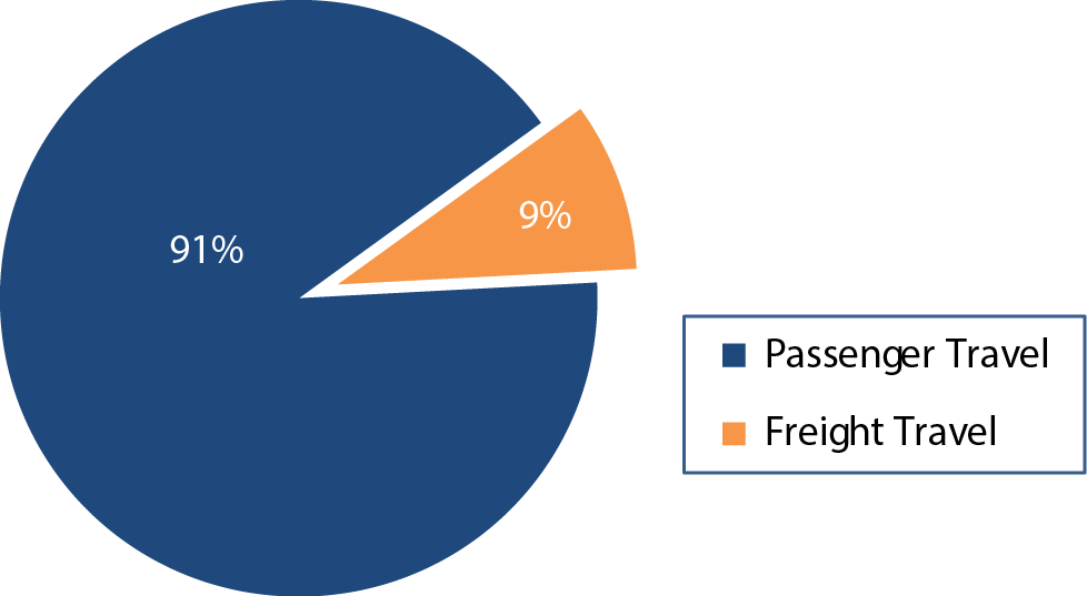
Source: Highway Performance Monitoring System.
The movement of people constitutes the vast majority of travel within the Nation's transportation system. Estimates from the Highway Performance Monitoring System show that 91 percent of the miles traveled in the United States are by passenger vehicles (see Exhibit 1-1).
Population changes, in both demographics and geographic location, historically have had significant impacts on the size and distribution of travel demand. The growth of the suburbs, and women entering the workforce are examples of influences demographic shifts can have on increasing travel.
Today, the U.S. population is undergoing changes in age distribution, racial and ethnic composition, migration, and immigration that affect the way we travel. In addition, advancements in information communication technologies, global positioning systems (GPS), sensors, and automation are affecting the personal travel experience.
Travel Trends
The past decade has experienced a shift in trends of vehicle ownership, vehicle miles traveled (VMT), and licensing rates, especially among teens and young adults. The number of registered vehicles rose from 111.2 million to 235.1 million between 1970 and 2013, but the number of cars per person peaked in 2008. Approximately 8.7 percent of households have no vehicle.
According to the Highway Performance Monitoring System, total VMT peaked in 2008 and per capita VMT peaked in 2004. Both have since decreased and leveled off (see Exhibit 1-2).
Licensing rates for teens and young adults have declined since the 1980s. In 1978, 46 percent of all 16-year-olds (1.9 million) and 97 percent of all 24-year-olds (3.8 million) had driver's licenses. In 2012, the rates dropped to 28.2 percent for 16-year-olds (1.2 million) and 83.4 percent for 24year-olds (3.6 million). This downward trend, which began well before the December 2007 to June 2009 recession, suggests that other factors could explain declining rates, such as the effects of graduated licensing and youth attitudes about driving (see Exhibit 1-3).
Exhibit 1-2 Per Capita Vehicle Miles Traveled, 1987—2012
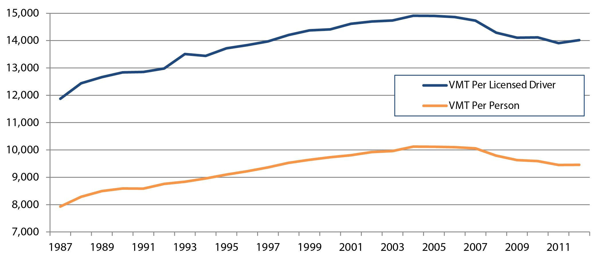
Source: Highway Performance Monitoring System.
Exhibit 1-3 Licensing Percentages for 16- and 24-year olds, 1978—2012
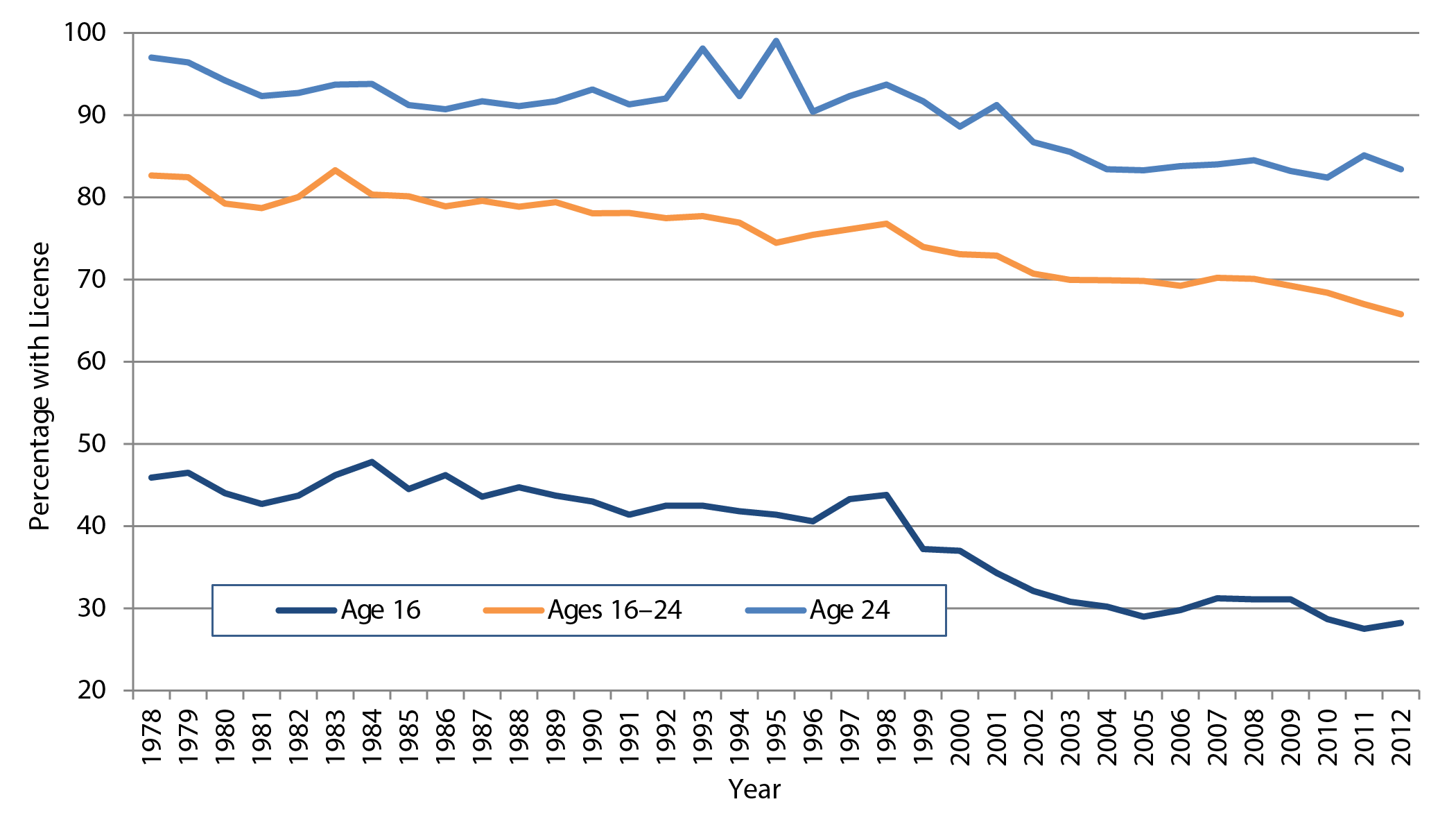
Source: Highway Statistics, Table DL-20.
Person Miles Traveled and Mode Share
Based on data available from the National Household Travel Survey (NHTS), person miles of travel (PMT), which includes vehicle and nonvehicle travel, declined less between 2001 and 2009 than VMT. Average vehicle occupancy decreased over this period but was more than offset by increases in nonvehicle travel. Nonvehicle miles include travel by modes other than personal vehicle (with the exception of car pools), including all public transportation, bike, walk, ferry, and air travel (see Chapter 11 for information on bicycle and pedestrian travel). While trips in private vehicles declined from 2001 to 2009, transit trips increased (see Exhibits 1-4 and 1-5).
Exhibit 1-4 Per Capita Daily Passenger Miles Traveled and Vehicle Miles Traveled, 1977—2009
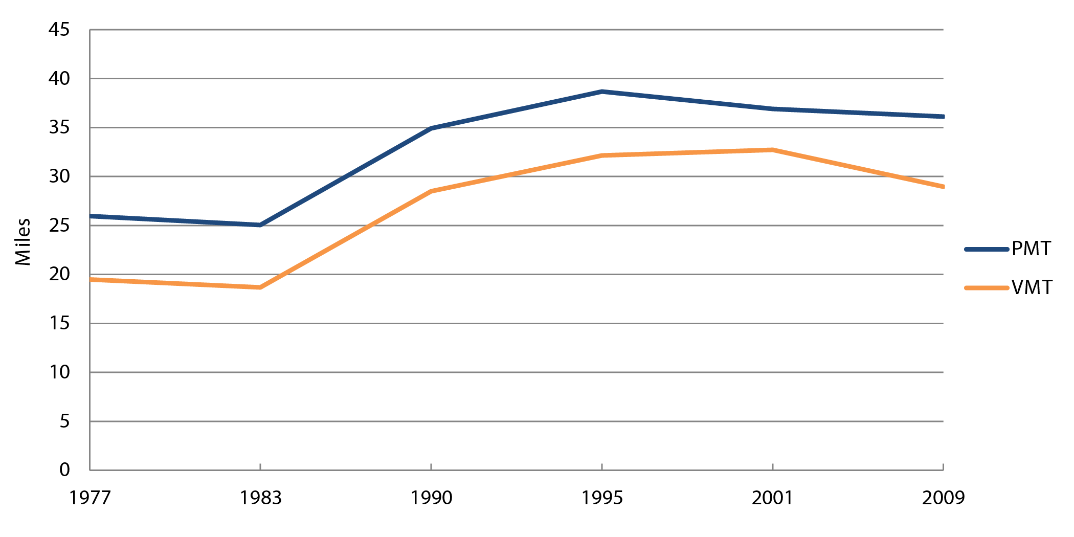
Source: National Household Travel Survey.
Exhibit 1-5 Percentage Change in Trips by Travel Mode, 1990—2009
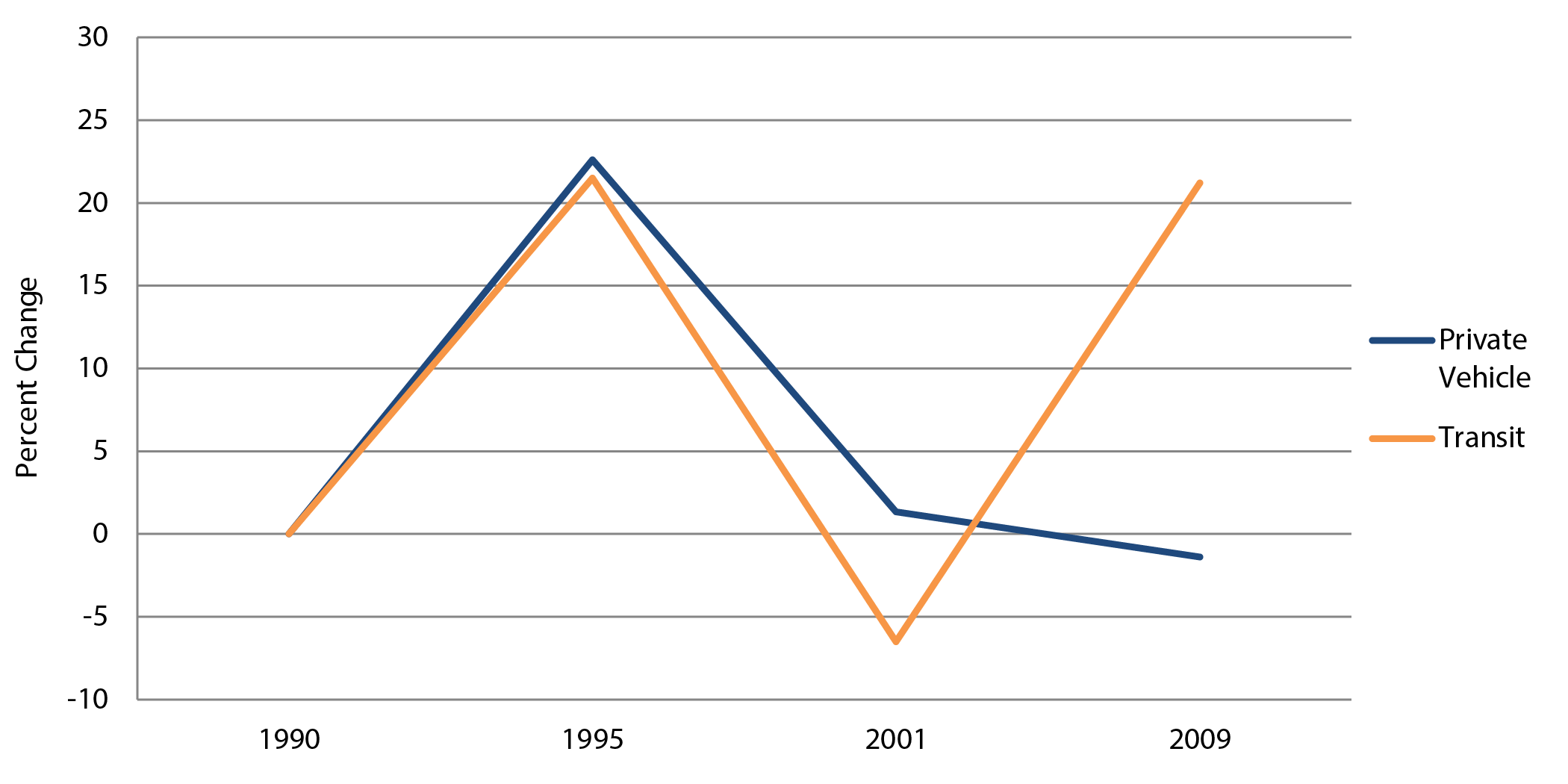
Source: National Household Travel Survey.
Where a person lives influences his or her mode choices. In densely populated areas, where public transportation is easily accessible, a large percentage of the public is likely to use the services. In New York City, for example, more than 50 percent of the population commutes to work using public transit (based on the metropolitan statistical area defined by the U.S. Census Bureau). As private vehicle travel has decreased in the past decade, use of public transit has increased; this shift has occurred, however, primarily in metropolitan statistical areas with a population of 500,000 and higher. Population density also plays a role in the use of other travel modes: The highest percentages of households without a vehicle occur within areas having population density of 10,000 or more per square mile. In addition to location, income influences mode choice. Lower-income households are less likely to own a vehicle. Individuals living in lower-income households and new immigrants are more likely to carpool, take transit, walk, or bike. As these populations continue to migrate from city centers to suburban locations, local area transportation agencies should consider the need for travel options in these areas.
Trip Purpose

Data from the NHTS and comparable predecessor surveys are available for 1969, 1977, 1983, 1990, 1995, 2001, and 2009. The next NHTS will be conducted in 2016.
Understanding why a person makes a trip provides transportation planners and policy makers the knowledge to better understand and anticipate travel volumes and demand and the needs of different traveling populations. For instance, aging populations might engage in more social and recreational travel, which can contribute to congestion during off-peak hours. Younger populations might rely on public transit to get to school or work places, emphasizing the need for reliable services to these destinations.
The NHTS is the only national data source that asks the American public why they took a given trip. Purposes of trips are classified into several categories: getting to or from work, shopping, running family or personal errands, and making social or recreational trips.
From 2001 to 2009, travel for all trip purposes declined or remained stagnant. Travel to work showed a 10percent decrease in miles and a 7-percent decrease in number of trips. American household travel for family or personal errands decreased by 13.9 percent and the length of trips for such errands dropped by 10 percent compared to 2001. In addition, daily PMT for social and recreational purposes declined by 9.5 percent between 2001 and 2009 (see Exhibit 1-6).
Of all trip purposes, discretion is greatest for traveling for family and personal errands and social/recreational trips. As non-work travel comprises a large percentage of daily travel, further research might be needed to examine whether the reductions from 2001 to 2009 were due primarily to economic reasons or to demographic and lifestyle changes among the American public.
Exhibit 1-6 Average Annual Person Miles and Person Trips per Household by Trip Purpose1
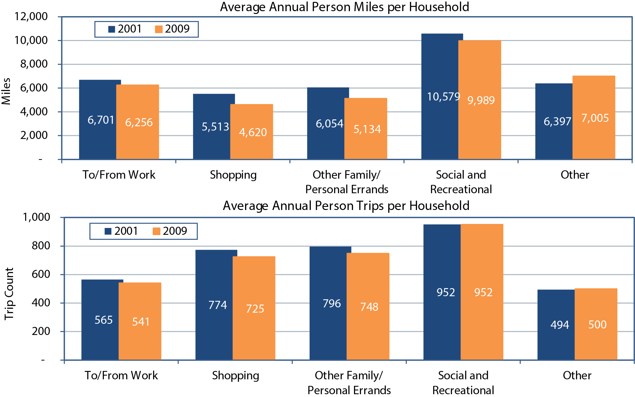
1The travel of children aged 0—4 years old is excluded from 2001 NHTS data to make it compatible with other years.
Sources: 2001 and 2009 NHTS.
Overall Population Trends
Between 1970 and 2013, the population of the United States increased by 53 percent , from 203 million to 316 million. By 2050, the U.S. population is projected to be just under 400 million. The annual rate of growth has declined in recent years to approximately 0.7 percent in 2013, the lowest growth rate since 1937. The rate is expected to continue to drop and by 2050 is projected to be 0.5 percent . Even though the growth rate is declining, the overall increase in population will result in an increase in total travel and an increased amount of freight being moved even if the miles and freight per person stabilizes or declines.
Aging Population
For the coming decades, the older population of the United States is expected to experience considerable growth. Most researchers expect the "baby boom" generation to enjoy increased longevity and to drive more miles than today's older adults. Currently, the number of people aged 65 years and older is approximately 40 million, and they account for 13 percent of the population. By 2050, this age group will double and account for 20 percent of the population, with the most significant increases occurring in the 85 years and older age group (see Exhibit 1-7).
Exhibit 1-7 Population Age Structure, 1960, 1990, and 2020
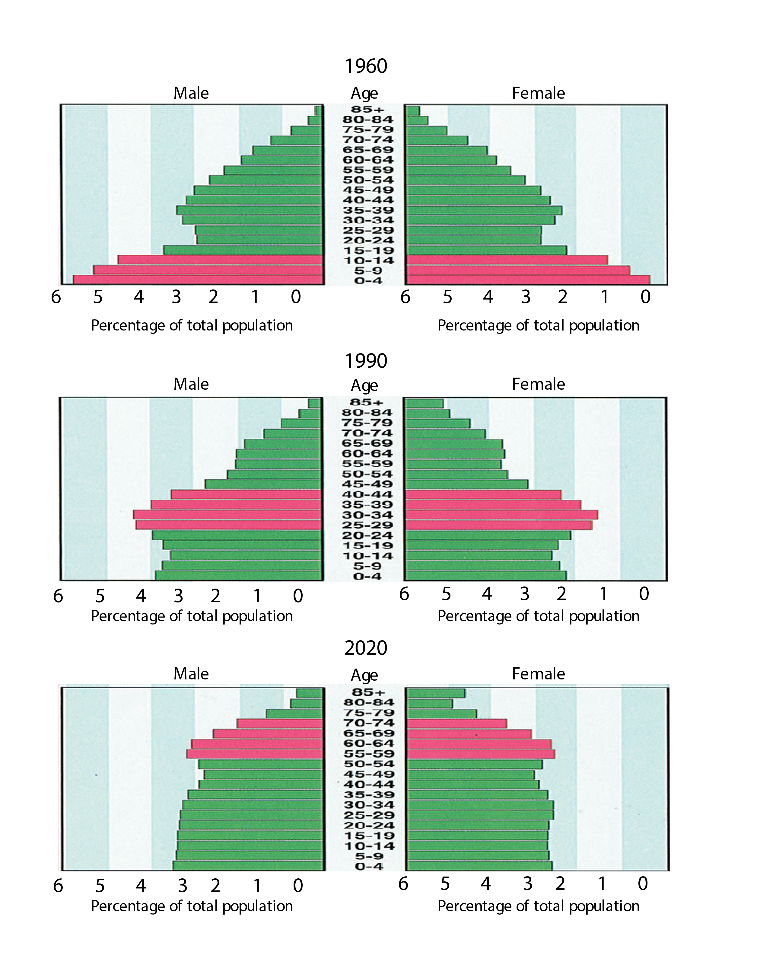
1Pink-shaded bars represent baby boomers.
Source: U.S. Bureau of the Census.
As the U.S. population ages, the percentage of older people continuing to work and drive will increase. Although some of the baby boom generation will retire, some will switch to part-time work, second careers, or volunteer activities. At the same time, the increase in the aging population also will result in an increased number of nondrivers requiring alternative means of mobility.
Daily patterns of travel shift with age. The proportion of travel for shopping, recreation, and other purposes (including medical appointments and to visit friends) increases as people age. More than 60 percent of daily travel by older adults occurs between 9 a.m. and 4 p.m., compared to young adults whose travel peaks during three distinct periods: morning (7 a.m. to 8 a.m.), midday (12 noon to 1 p.m.), and after work (5 p.m. to 6 p.m.). The growth in the older population could add significantly to midday travel.
Diversity
Not only is the population aging, it is also becoming more ethnically diverse. Minority groups, which made up 12 percent of the total population in 1970, have increased to 27 percent in recent years. In 2050, this percentage is expected to increase to 50 percent , with no single race or ethnic group having the majority (see Exhibit 1-8).
Exhibit 1-8 Racial and Ethnic Composition of the United States, 1970—2050
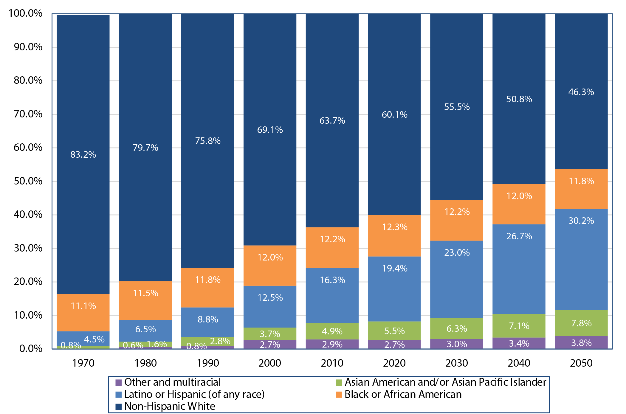
Sources: Data for 1970 and 1980 obtained from Statistical Abstract of the United States; data for 1990, 2000, and 2010 obtained from the U.S. Census Bureau; data for 2020 through 2050 came from the U.S. Census Bureau Population Projections by Race and Ethnicity (2008).
Immigration has a significant impact on national, regional, and local transportation needs. New immigrants travel differently than long-term residents because they are less likely to own a vehicle and more likely to depend on other modes of travel such as carpooling, public transit, walking, and bicycling.[1] Because of this, immigration places a different set of demands on the transportation system, and, for the first time since 1920, immigrants comprise more than 12 percent of the U.S. population. Although the immigrant population (even at the projected 2050 levels) is not substantial enough to influence national VMT and PMT projections significantly, regions in the United States with high levels of immigration will experience a significant shift in travel demand and forecasting assumptions.
Trends in Household Size
Historically, the number of households has increased much faster than the total population. Although the overall population of the United States increased by 270 percent from 1900 to 2000, the total number of households grew from 16 million in 1900 to more than 105 million in 2000, an increase of 561 percent .
Between 1960 and 2013, total households increased from roughly 53 million to more than 122 million, while the average household size decreased from 3.33 to 2.54 persons per household. The major reason for this rapid household growth is changing household structure.
Nationally, household size has been steadily declining for decades, trending toward smaller families and more single-person households. Average household size has decreased since 1970, when the average household had 3.11 persons. In 2010, it had 2.63, a slight increase from 2000. Even though the proportion of nuclear family households (those with married parents and at least one child under 18 years of age) has declined, the proportions of all other household types have increased: families without children at home, single-person households, and households of unrelated persons. Smaller household size increases the number of trips for some and reduces mobility for others due to limits in transportation access (e.g., shared vehicles, carpooling).
Income and Labor
Income
Between 2000 and 2009, U.S. transportation costs increased at nearly twice the rate of incomes. In the United States, personal income has been the most important predictor of personal travel demand, although these trends have begun to diverge over the past 10 years. Other economic factors, including employment levels (and the resulting commuting patterns) and transportation costs such as transit prices, fuel prices, and automobile prices (including vehicle operating costs), also affect transportation decisions and vehicle utilization rates. Due to this direct and longstanding influence on personal travel, economic and employment trends are an important consideration in transportation policy.
On average, U.S. citizens spend 20 percent of their income on travel-related expenditures, and transportation is the second largest expenditure for households after housing, although this varies by location and income. Households located in more diffuse, automobile-dependent regions are estimated to spend 25 percent of their income on transportation, while households located closer to employment and other amenities spend an estimated 9 percent of household income on transportation.
Poverty
The current national poverty rate is close to 15 percent and by 2020 is expected to decline to around 14 percent . Despite this decline, analyses suggest many years will pass before it returns to rates experienced before the December 2007 to June 2009 recession.
Both unemployment and poverty rates respond to changes in workforce location and geographic influences. For several years, the geography of poverty has been shifting from urban to suburban, presenting new transportation-related challenges. The economic gap between high- and low-income working families is growing. In 2011, 46.2 million people were poor-22.5 percent of them working poor-and they comprised 7 percent of the total work force. The working poor spend a much higher portion of their income on commuting and use public transit, carpooling, biking, and walking more frequently than higher income workers do.
Unemployment and Labor Force Participation
Although related to economic factors, workforce composition and distribution affect travel-related trends in different ways. The availability and location of employment have a significant impact on where people live and how they commute to work. Commuting to work constitutes approximately 16 percent of all person trips and 19 percent of all PMT. For roadway travel, commuting comprises 28 percent of household VMT and for transit systems, 39 percent of all transit PMT. Although the average commuting time has remained relatively consistent at 25 minutes, typical commuting patterns are becoming more complex and are likely to involve more trip chains that incorporate stops along the way that are not related to work.
In 2012, the unemployment rate was 8.1 percent . The rate has declined since the December 2007 to June 2009 recession but is still higher than it has been since the 1990s. The rate, however, is expected to continue to decline. Furthermore, after a long-term increase, the overall labor force participation rate has declined in recent years. Although a sharp rise in participation occurred among individuals aged 55 and older, the largest drop was in 16-to 24-year-olds and especially in teenagers. The driving factors for this drop include increased rates of school enrollment, a slower than average labor market recovery, and higher competition for available jobs (from older workers and recent immigrants). Looking forward, the rate of labor force participation is expected to continue decreasing through at least 2022 (see Exhibit 1-9).
Exhibit 1-9 Labor Force Participation Rates, 1947—2012 and Projected Rates for 20221
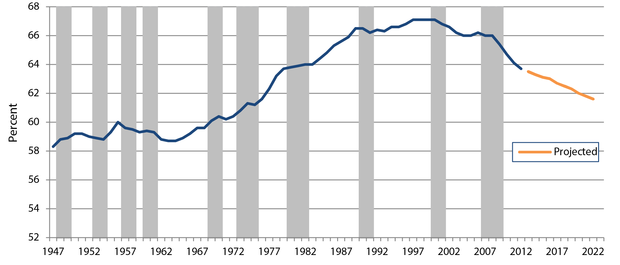
1Shaded regions represent recessions as designated by the National Bureau of Economic Research. Turning points are quarterly.
Source: U.S. Bureau of Labor Statistics.
Geography
Where people live, work, and recreate and how they travel are intimately related to their place of residence. For example, living in a dense urban area, where origins and destinations are closer together and public transit is available, slows automobile speeds, increases parking costs, and provides more opportunities to travel by other modes.
The distribution of the population significantly influences the amount of freight, business, and personal travel in a given area. As metropolitan regions continue to expand, maintaining and improving our Nation's transportation system is critical.
Regional Migration
Census projections through 2030 show that population growth will continue to be sharply skewed geographically, with almost half the national growth occurring in three States: Texas, Florida, and California. These three States account for most of the growth that is occurring in the South and West, contributing to a projected 88 percent in growth. In comparison, about half the States in the Nation have shown slow or stagnant growth (see Exhibit 1-10). Such a sharply skewed population distribution will make defining an equitable national transportation program difficult to achieve. Additionally, increases in both freight and passenger travel are likely to continue to concentrate in specific geographic areas, adding to system performance and maintenance issues.
Exhibit 1-10 Regional Migration and Growth
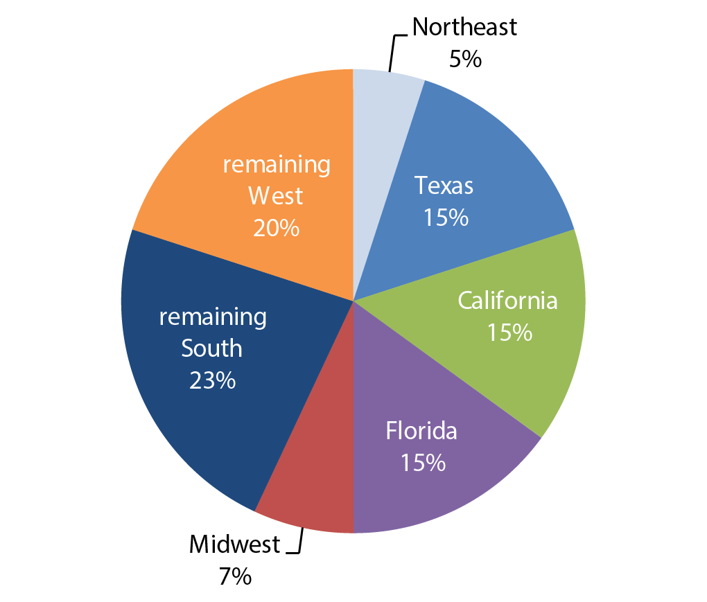
Source: U.S. Census Bureau.
Population change is due to both migration and immigration. Migration has slowed in the United States over the past few years; in fact, the 5-year move rate for 2010 was the lowest in history at 35.4 percent (U.S. Census Bureau, Geographic Mobility: 2005—2010). People in their 20s have the highest move rate (65.5 percent ), followed by the unemployed (47.7 percent ). The South was the only region to show a significant gain due to migration from 2000 to 2010; the Northeast and Midwest lost 2.6 million in population to the southern and western United States.
Knowing the distribution of new immigrants across our Nation's cities and States helps us better understand the transportation needs of people in the geographic locations where immigration levels are very high. New immigrants are still more likely to take up residence in the "Big Six" immigrant magnet States: California, New York, Texas, Florida, Illinois, and New Jersey. These States accounted for 65 percent of the foreign-born population in 2012.
Another notable trend is the dispersion of new immigrant populations to other States, including Georgia, North Carolina, Arizona, Washington, and Virginia. Over the past 5 years, Georgia has experienced a 38-percent increase in its foreign-born population. The State of Washington has experienced a 24-percent increase in the number of foreign-born residents since 2000.
By 2050, the immigrant population in the United States is projected to reach 68 million, 16.2 percent of the total population. High-series projections from the census estimate the immigrant population to reach 114 million in 2050.
Increased Urbanicity
The Bureau of the Census does not provide detailed metropolitan population growth projections, but substantial evidence from the past 100 years, and certainly over the past 50 years, indicates what the direction might be.
Most of the Nation's growth has occurred in suburbs. Today, the suburbs contain more than half the national population. Just over half of young people (ages 20—34) live in suburban areas. Youth are more commonly taking up residence in suburban neighborhoods, particularly in new developments. These developments are often located on the fringes of metropolitan areas, where access to public transportation can also be sparse (see Exhibit 1-11). Additionally, low-income families are moving from city centers to more suburban locations. In 1970, suburbs housed 25 percent of the poor, and by 2010, it was 33 percent .
Exhibit 1-11 Percentage Point Change in Young Adult Population (Ages 20—34 Years) by Neighborhood Type, 2000—2010
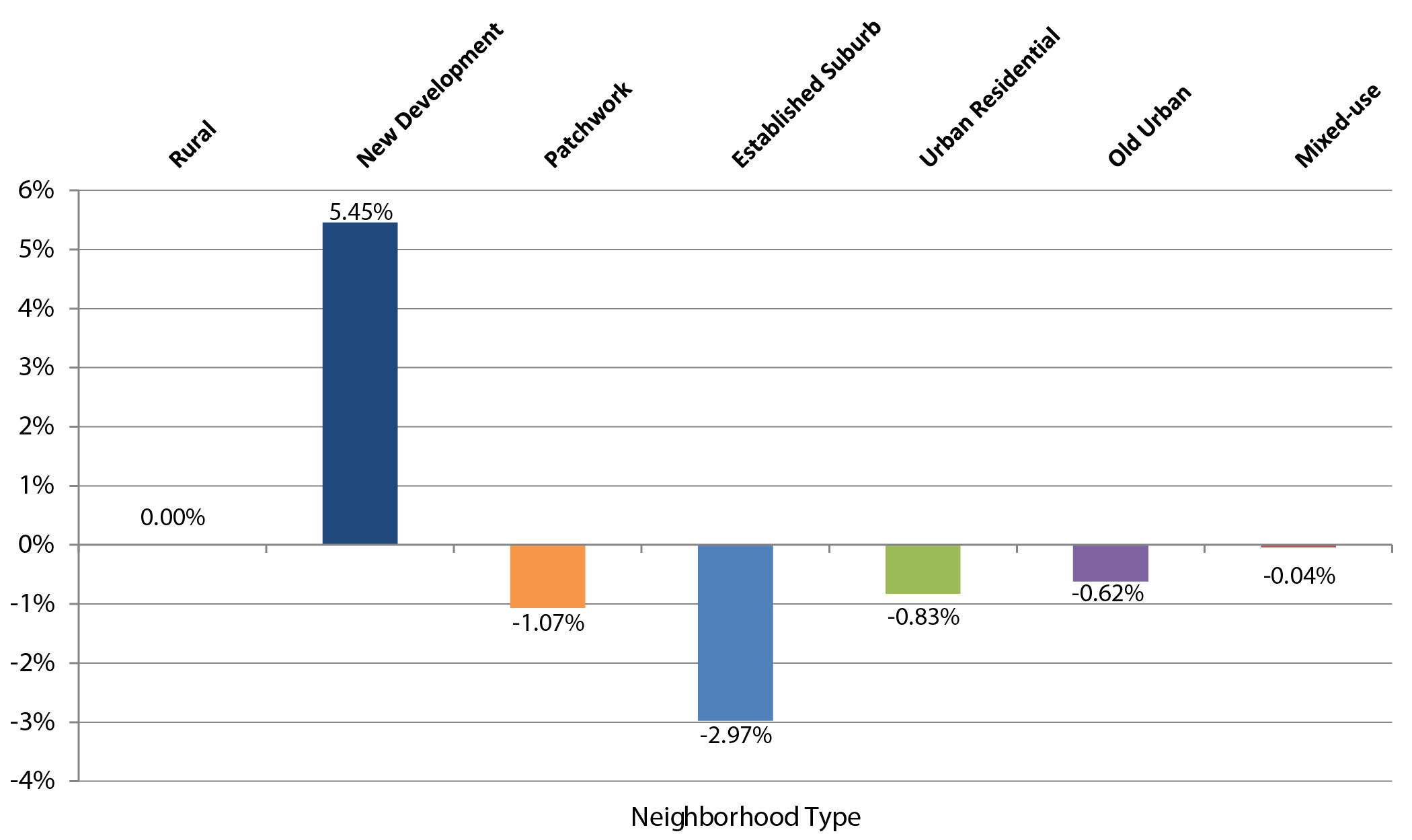
Source: Typecasting Neighborhoods and Travelers: Analyzing the Geography of Travel Behavior Among Teens and Young Adults in the U.S., Institute of Transportation Studies, UCLA Luskin School of Public Affairs, 2015.
A large part of the "suburban" growth has occurred because rural areas are becoming incorporated into neighboring metropolitan areas. Currently, the rural population is declining in terms of both the percentage of U.S. population and in actual population size. More than 40 rural counties were classified as metropolitan in the 2000 census.
Across most communities in the country, travel differences between suburban and urban residential areas are surprisingly small; significant differences occur, however, in rural areas and in old urban neighborhoods. In rural areas, VMT is significantly higher, which reflects the need for residents to travel longer distances to destinations using a vehicle.
In old urban neighborhoods, residents make fewer trips, travel fewer miles, are less likely to have a license, and are more likely to walk or take public transit. Old urban areas tend to have more households without vehicles and better access to transit services, compared to other neighborhoods. Nearly three-fourths of old urban neighborhoods are located in New York and Los Angeles.
Growth in Megaregions
Between 2000 and 2010, urban population growth (12.7 percent ) outpaced overall national growth (9.7 percent ). More than 50 percent of U.S. population growth through 2050 is projected to occur in the Nation's largest metropolitan areas.
As cities grow in size and population, a network across metropolitan centers is created with environmental, economic, and infrastructural relationships. These "megaregions" often cross county and State lines-linked by both transportation and communication networks. Many experts believe that by 2050, 75 percent of the U.S. population will live in megaregions and more than half the Nation's population growth will occur there.
At present, 11 emerging megaregions have been identified. They include the Northeast, Florida, Piedmont Atlantic, Gulf Coast, Great Lakes, Texas Triangle, Arizona Sun Corridor, Front Range, Cascadia, Northern California, and Southern California.
Megaregions span State and political boundaries, which will require substantial coordination among several entities in planning future transportation systems. Regional economies are likely to become so interwoven that the transportation system will have to endure dramatic increases in both freight and passenger travel. The northeastern corridor, for instance, is expected to experience a 50-percent growth in rail traffic by 2050 (see Exhibit 1-12).
Exhibit 1-12 Emerging Megaregions of the United States
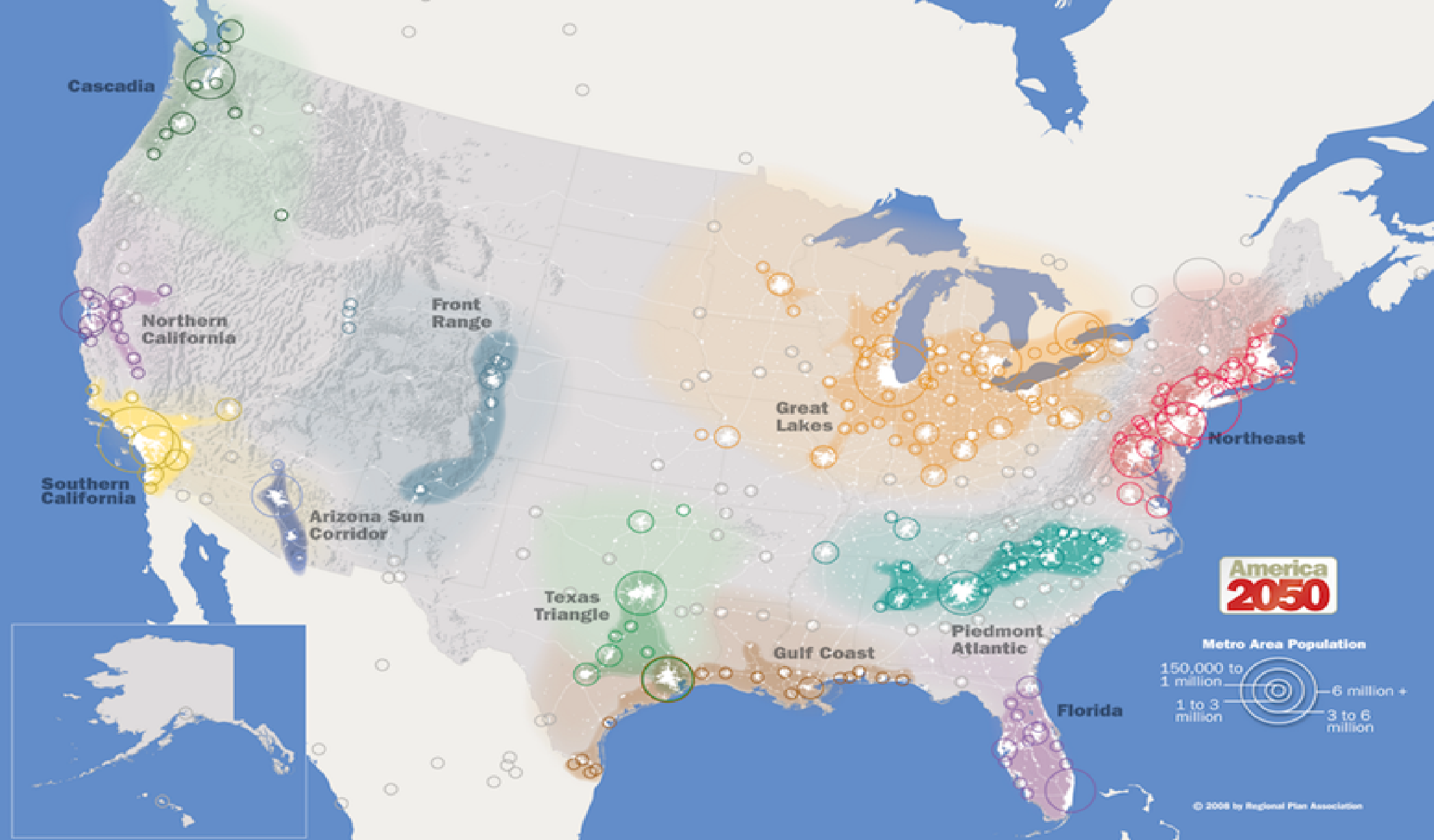
Source: http://www.america2050.org/maps/
Technological Trends and Travel Impacts
Over the past two decades, advancements in Information Communication Technologies have not only changed the way we communicate, but also the way we travel. Our lifestyles and travel decisions are influenced by our need for time. New technologies have enabled us to do things faster, with greater accuracy and more options.
We live in the age of the "informed traveler." Our understanding and use of the transportation system has grown with the availability of travel apps and real-time data. We now know how best to reach our destination, how long the trip will take, and how to pay for it easily, if required. If we need a vehicle, we can find one online and complete the transaction in minutes. We can know ahead of time that traffic is unbearable and change our travel plans to save time.
This section discusses a few technological advancements that have influenced our travel decisions and the way we travel, including GPS use in travel data collection, payment systems, the rise of the sharing economy organizations and businesses, and telecommuting.
Using GPS and Smartphones to Collect Personal Travel Data
Over the past several years, interest has grown in advancing data collection techniques to help reduce survey burden and increase data accuracy. Emerging technologies to collect travel data, such as GPS and smartphones, are becoming more widely used as a means not only to collect location data, but also to obtain additional information about the personal trip-making experience.
Made possible by sensors, smartphones can detect motion, speed, and location via cellular network or wireless fidelity (Wi-Fi), and proximities to nearby objects. Most phones today are equipped with accelerometers that measure linear speeds. The raw data are fed through software programmed with a trip-detection algorithm that can determine whether a person is traveling by car, bike, taking public transit, or walking.
In addition to mode detection, GPS or other network-based services can use location data to identify frequently visited locations, including arrival and departure times. Land use information obtained from GIS maps can be used to determine most frequently traveled routes and details about the transportation system infrastructure, such as the availability of sidewalks.
All these data can be collected passively, requiring nothing from the participant except to carry the smartphone and keep it charged. When more detail is needed about a person's trip-making experience, such as the purpose of the trip, reasons for route selection, or travel party size, a follow-up survey can be programmed into a phone application that prompts the user to answer questions about trips taken.
Since the first FHWA-sponsored study in Lexington, Kentucky in 1996, GPS has been used to collect data on travel behavior in other areas of the country, including Portland, Oregon; Chicago, Illinois; San Francisco, California; Austin, Texas; and South Florida. For the NHTS, several States will be integrating GPS technologies into add-on survey work as part of the national collection. Integrating GPS and smartphone technologies into travel behavior surveys is quickly becoming a more common practice among metropolitan planning organizations and State Departments of Transportation; however, hurdles to overcome remain, such as the cost of acquiring and distributing smartphones and how best to extend phone battery life during the survey period.
Electronic Payment Systems
Advancements in the area of payment systems have made paying for transportation more convenient. These advancements are important to State Departments of Transportation and local transit agencies that are facing increasing pressures to reduce operating costs and increase revenues, in addition to improving customer convenience and quality of service. Integrated transportation payment systems lead to greater efficiencies, provided these systems are secure, preserve privacy, and do not lead to fraud.
Technologies for integrated transportation payment systems include the use of magnetic stripe cards, "smart cards," and electronic toll collection transponders and systems that enable the user to make a payment electronically. Value can be added to the card or device, and the cost of a trip is deducted for each trip. Where available, the card or device can act as a pass that allows the user unlimited access for a certain period of time, typically a month. The card or device can also contain client information.
The advent of electronic tolling has helped alleviate congestion surrounding toll facilities by allowing for ease of payment. Electronic tolling that involves variable pricing (pricing that is based on the time of day, level of service, or other factors) might shift traffic away from peak hours. A New Jersey study found a small, but statistically significant, shift in car traffic to prepeak hours in the morning (5 a.m. to 6 a.m.) and afternoon (3 p.m. to 4 p.m.), especially among younger drivers and those who come from lower income households.[2] Additionally, traffic could be diverted to alternative non-tolled routes.
Integrated transportation payment systems commonly used in public transportation include magnetic stripe cards and smart cards. Magnetic stripe cards are inexpensive, reliable, and have a high customer acceptance. These cards, which can store value over time, can be used throughout multiple transit networks. Trip origins and destination information can be recorded on the cards.
Smart cards are made of plastic, similar to a credit card and contain microprocessors and memory chips with wireless communication capabilities.[3] Smart cards, sometimes called integrated circuit cards, are similar to magnetic stripe cards but store the information on an embedded microcomputer chip rather than the stripe. Smart cards have been used in a range of applications, including toll and parking payments, Internet access, and mobile commerce.
These technologies make the use of public transportation more convenient, possibly encouraging ridership. Riders no longer need to carry correct change to ride the bus or keep track of multiple train tickets. Increasingly, riders who transfer between modes of public transportation no longer need to carry a transfer pass, as transfer passes are often automatically loaded onto smart cards.
Innovations in smartphone technology and in the financial service industry have provided additional convenience to paying for transportation. Paying for services by mobile phone is already a common practice abroad and is becoming a more frequent method of payment in the United States. The American Public Transportation Association Universal Transit Farecard Standards is one example of a program that actively promotes the Contactless Fare Media System Standard[4] for use in contactless fare systems throughout North America. Additionally, exciting developments are occurring in the contactless payments industry that will simplify the future of transit fare collection. These include using contactless bankcards, mobile devices, and identification credentials to pay for transit fare.
The added convenience that integrated transportation payment systems bring to transportation users and the industry is not the only benefit of using these systems. The wealth of data that can be acquired from trip tracking provides planning agencies and other transportation professionals with the information necessary to understand the needs and value of existing systems more completely.
Sharing Economy
The rise of sharing economy organizations and businesses is having a marked influence on the way people travel. In certain areas, travelers are more often choosing to forgo car ownership and rely on other means of travel, among them, car and ridesharing services.
Increasing use of the Internet and mobile phones and the development of enabling technologies, such as social media platforms, open data sources, and phone applications, have created a market that makes goods and services easier to share and more accessible to a larger audience. Forbes estimates that the revenue flowing through the share economy will surpass $3.5 billion in 2013, with growth exceeding 25 percent .[5]
In the share economy, owners make money from underused assets, or the value of unused time that goods and services remain idle. Peer-to-peer car sharing, for instance, is a service that offers car owners the opportunity to rent out their personal vehicle. Mobile phone applications help facilitate the transaction by making the process quick and easy. Car owners who rent their vehicles using peer-to-peer services such as Relay Rides reportedly can make an average of $250 per month, and some make more than $1000.[6]
Many carsharing organizations have received startup grants and incentives from Federal, State, and local sources. FHWA's CMAQ (Congestion Mitigation and Air Quality) program provides funding to States for eligible activities that reduce VMT or encourage the use of alternative fuels. The State of California, for instance, has enacted legislative initiatives to support carsharing by reducing barriers that owners might face when sharing their vehicles and has worked with local governments to provide exclusive use of onstreet parking for carsharing vehicles.[7]
The continuing growth of the sharing economy could affect personal travel. Studies have shown that carsharing programs have mixed effects on VMT. In some cases, households have slight increases in VMT, but households that lose one or all vehicles show substantial reductions in VMT. These households learn to adapt to a new travel lifestyle that leads to modal shifts facilitated by car sharing.[8] Carsharing vehicles typically are also newer and more fuel efficient than the average privately owned vehicles, which helps decrease emissions, even if miles are not reduced (see Exhibit 1-13).[9]
Ridesharing service companies are connecting drivers to riders and coordinate rides in minutes using mobile phone, GPS technology, and online payment systems. Unlike traditional taxis, these companies boast faster and cheaper service, without the need for hailing.
As the public continues to adapt to new technologies and ways of travel, modal shifts are likely to increase, primarily among nonwork trips (as commute and short trips are typically traveled by walking, biking, and public transit use[10]). The future of the traveling public will be influenced by sharing economy practices and the effect they could have on increased modal options.
|
||||||
|---|---|---|---|---|---|---|
| Study | Study Location | Study Year(s) | Difference in VMT | Difference in Emissions | Difference in Gasoline Consumption | |
| After vs. before joining carsharing | ||||||
| Martin and Shaheen, 2011a | Multiple cities | Varies—2008 | -26.9% | -34.5% | N/A | |
| Cervero et al., 2007 | San Francisco Bay area | 2001—2003 | Not significant | N/A | -36.5% | |
| 2001—2005 | -32.9% | N/A | -59.5% | |||
| Carsharing members (or pre-members) vs. non-members | ||||||
| Cervero et al., 2007 | San Francisco Bay area | 2001 (pre-launch) | -33.1% | N/A | -65.1% | |
| 2003 | -66.4% | N/A | 89.9% | |||
| 2005 | -68.2% | N/A | 90.3% | |||
| Source: Boarnet, Handy, Lovejoy, Impacts of Carsharing on Passenger Vehicle Use and Greenhouse Gas Emissions, California Air Resources Board, 2013. | ||||||
Telecommuting
Someone who telecommutes or teleworks is most often working from home or a place other than their usual worksite. Over the past two decades, advancements in information communication technologies, increased access to broadband services, and changes in workplace policies have made the ability to telework a possibility for those whose jobs are telework eligible.
In 2010, 13.4 million people worked at least one day at home per week, an increase in more than 4 million people (35 percent ) in the past decade.[11] In the past three decades, the number of teleworkers has almost tripled, from just 2 million in 1980 to 6 million in 2010.[12] As of 2009, approximately 2.3 percent of the total workforce telecommutes at least one day a week (see Exhibit 1-14).
Exhibit 1-14 Teleworking Population, 2005 and 2009
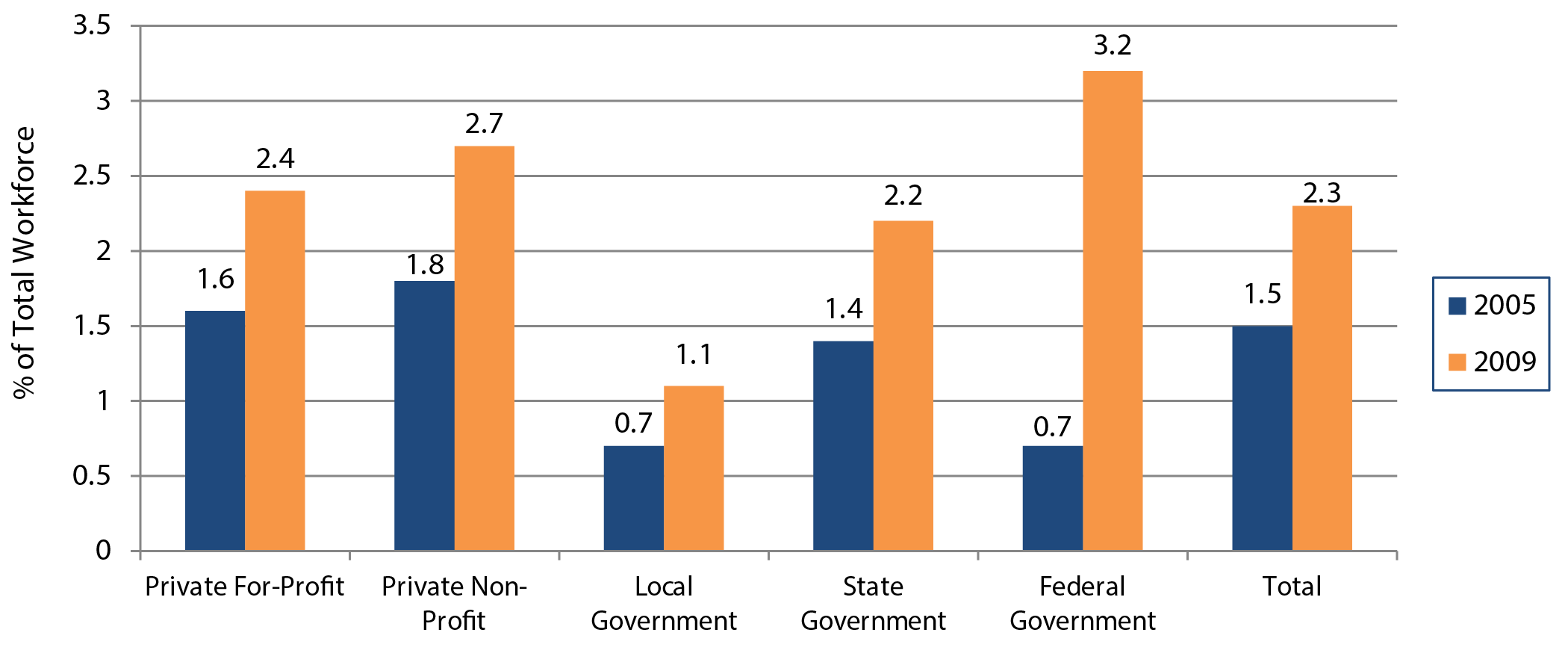
Source: 2005 and 2009 American Community Survey Collected by Telework Research Network.
Telework Relative to Transit
In certain urban areas of the country (primarily in the West and Southwest), teleworkers outnumber transit commuters.
Source: Potential Impacts of Increased Telecommuting on Passenger Travel Demand, National Surface Transportation Policy and Revenue Study Commission, January 2007
Teleworkers are more likely to be self-employed or work in the private sector. Common occupations associated with home-based telework include jobs in the business and finance fields. The number of telework-eligible positions in the computer, scientific, and engineering fields is growing. More than 50 percent of teleworkers have a bachelor's degree or higher. The largest growth in teleworking by census region in the United States has occurred in the South and West, where overall worker growth was also greater (see Exhibit 1-15).
|
||
|---|---|---|
| Rank | Metropolitan Statistical Area | percent |
| 1 | Boulder, CO | 10.9 |
| 2 | Medford, OR | 8.4 |
| 3 | Santa Fe, NM | 8.3 |
| 4 | Kingston, NY | 8.1 |
| 5 | Santa Rosa-Petaluma, CA | 7.9 |
| 6 | Mankato-North Mankato, MN | 7.7 |
| 7 | Prescott, AZ | 7.6 |
| 8 | St. Cloud, MN | 7.6 |
| 9 | Athens-Clarke County, GA | 7.5 |
| 10 | Austin-Round Rock-San Marcos, TX | 7.3 |
| Source: American Community Survey, 2010. | ||
The opportunity to telework benefits workers and companies alike. It adds flexibility to the workday, which helps families and individuals better manage the responsibilities of daily life without being confined to a workplace location. It also saves workers time from the daily commute, which for some, might add up to several hours a week. Companies and public agencies have found that giving employees opportunities to telework can increase productivity and increase employee retention.[13] Teleworking has become an important part of workplace efforts to help employees balance work/life issues.
From the transportation perspective, telecommuting has become a component of many Transportation Demand Management (TDM) programs within State Departments of Transportation and metropolitan planning organizations to relieve congestion at the local/regional level during commute times. In urbanized areas, it can improve air quality by helping reduce emissions associated with traffic congestion.
Federal dollars from the CMAQ program can be used by State Departments of Transportation and metropolitan planning organizations to support telework programs that help reduce emissions. Private institutions have also provided funding to implement telework programs as part of local initiatives to reduce congestion and improve air quality. The Clean Air Campaign in Atlanta, Georgia,[14] for example, has trained thousands of teleworkers and has worked with almost 300 companies to institute telework policies.
On a nationwide scale, the impact of telecommuting on total congestion is difficult to evaluate due to a myriad of factors associated with personal travel decisions. Some might argue that, although telecommuting can reduce peak-hour trip making or VMT, it has no effect on total trip making or total VMT,2 as teleworkers could travel to other destinations throughout the workday. Various studies have shown, however, that increases in trip making by teleworkers are related more so to individual differences in workers, and are not a result of the act of teleworking. For instance, high-income teleworkers still show more trip making during the workday than low-income teleworkers.[15] Because of the diversity of individuals who make up the workforce and differences in land uses and transportation systems from place to place, the success of telework programs in reducing congestion are best evaluated at the local or regional level.
Looking Forward
New technologies will continue to affect how people travel by increasing our knowledge of the personal trip experience and through increased system efficiencies that influence how we use our time. Changes to the transportation system are inevitable, as vehicle automation features to improve safety and trip reliability continue to gain a predominant place in the car market. In the future, travelers might no longer need to think as much about how to get there, but what to do along the way.
Freight Movement
The economy of the United States depends on freight transportation to link businesses with suppliers and markets throughout the Nation and the world. Freight affects nearly every American business and household in some way. American farms and mines use inexpensive transportation to compete against their counterparts around the world. Domestic manufacturers rely on remote sources of raw materials to produce goods. Wholesalers and retailers depend on fast and reliable transportation to obtain inexpensive or specialized goods. In the expanding world of e-commerce, households and small businesses increasingly depend on freight transportation to deliver purchases directly to them. Service providers, public utilities, construction companies, and government agencies rely on freight transportation to obtain needed equipment and supplies from distant sources.
The U.S. economy requires effective freight transportation to operate at minimum cost and respond quickly to demands for goods. As the economy grows over the next several decades, the demand for goods and the volume of freight transportation activity will increase. Current volumes of freight are straining the capacity of the transportation system to deliver goods quickly, reliably, and cheaply. Anticipated growth of freight could overwhelm the system's ability to meet the needs of the American economy unless public agencies and private industry work together to improve the system's performance.
Freight Transportation System
The Bureau of Transportation Statistics' (BTS) publication, Freight Facts and Figures 2015, shows the U.S. freight transportation system handled a record amount of freight in 2012. About 54 million tons of freight worth more than $48 billion was transported each day across all modes of transportation to meet the logistical needs of the Nation's 118.7 million households, 7.4 million business establishments, and 89,004 government units. This system includes nearly 10.7 million single-unit and combination trucks, more than 1.3 million locomotives and rail cars, and over 40,000 marine vessels. The system operates on almost 450,000 miles of Interstate, other limited-access, and arterial highways; nearly 140,000 miles of railroads; 11,000 miles of inland waterways and the Great Lakes-St. Lawrence Seaway system; and almost 1.75 million miles of petroleum and natural gas pipelines. The U.S. Army Corps of Engineers' Waterborne Commerce of the United States 2012 identifies 133 ports that handle more than 1 million tons of freight per year.
The freight transportation system is more than equipment and facilities. As reported in Freight Facts and Figures 2013, freight employment at for-hire transportation establishments currently is over 4.4 million workers in the United States. Truck transportation businesses comprise the single largest freight transportation occupation, employing more than 1.3 million workers. Other freight transportation and freight transportation-related occupations include rail and water vehicle operations, pipeline operations, equipment manufacturing, infrastructure construction and maintenance, and secondary support services.
Freight Transportation Demand
Freight movements in the United States take a variety of forms, from the shipment of farm products across town to the shipment of electronic devices across the world. These goods move to, from, and within the United States via the Nation's highways, railroads, waterways, airplanes, and pipelines, sometimes using a combination of two or more of the aforementioned modes to complete the trip. Due to the country's well-developed roadway network and the transport connectivity and flexibility the network provides, most freight moved to, from, and within the United States is transported by truck. Exhibit 1-16 shows a breakdown of freight movements by mode, measured by both tonnage and value of shipment.
|
||||
|---|---|---|---|---|
| Mode | Tons (Millions) | Percentage | Value (Billions of Dollars) | Percentage |
| Truck | 13,182 | 67.0% | 11,130 | 64.1% |
| Rail | 2,018 | 10.3% | 551 | 3.2% |
| Water | 975 | 5.0% | 339 | 2.0% |
| Air; Air and Truck | 15 | <0.1% | 1,182 | 6.8% |
| Multiple Modes and Mail | 1,588 | 8.1% | 3,023 | 17.4% |
| Pipeline | 1,546 | 7.9% | 768 | 4.4% |
| Other/Unknown | 338 | 1.7% | 359 | 2.1% |
Total1 |
19,662 | 100% | 17,352 | 100% |
|
1 Numbers may not add to totals due to rounding. The data are provisional estimates that are based on selected modal and economic trend data. All truck, rail, water, and pipeline movements that involve more than one mode, including exports and imports that change mode at international gateways, are included in multiple modes and mail to avoid double counting. As a consequence, rail and water totals in this table are less than other published sources. In addition, it should be noted that raw tonnage statistics does not take into account the distance these goods were moved. To use one example, a shipment, such as a shipping container, that is transported 2 miles by truck and 2,000 miles by rail is treated the same when measured by tonnage. Sources: U.S. Department of Transportation, Federal Highway Administration, Office of Freight Management and Operations, Freight Analysis Framework, version 3.4, 2014. |
||||
Exhibit 1-17 shows a map containing the tonnage information presented in the table in Exhibit 116 for truck, rail, and inland water shipments, plotted to the U.S. freight transportation network. Exhibit 1-18 shows the same information as in Exhibit 1-17, but includes only long-haul truck shipments on the National Highway System (NHS).
Much of the freight moved on the U.S. transportation system is transported by for-hire carriers-third-party carriers that serve a variety of customers. The Bureau of Transportation Statistics' Freight Transportation Services Index measures the output of services provided by for-hire transportation industries. According to the Bureau, this freight index correlates strongly with U.S. economic activity and helps illustrate the relationship between freight transportation and long-term changes in the U.S. economy. Exhibit 1-19 shows the annual Freight Transportation Services Index figures for recent years.
Exhibit 1-17 Tonnage on Highways, Railroads, and Waterways, 2010
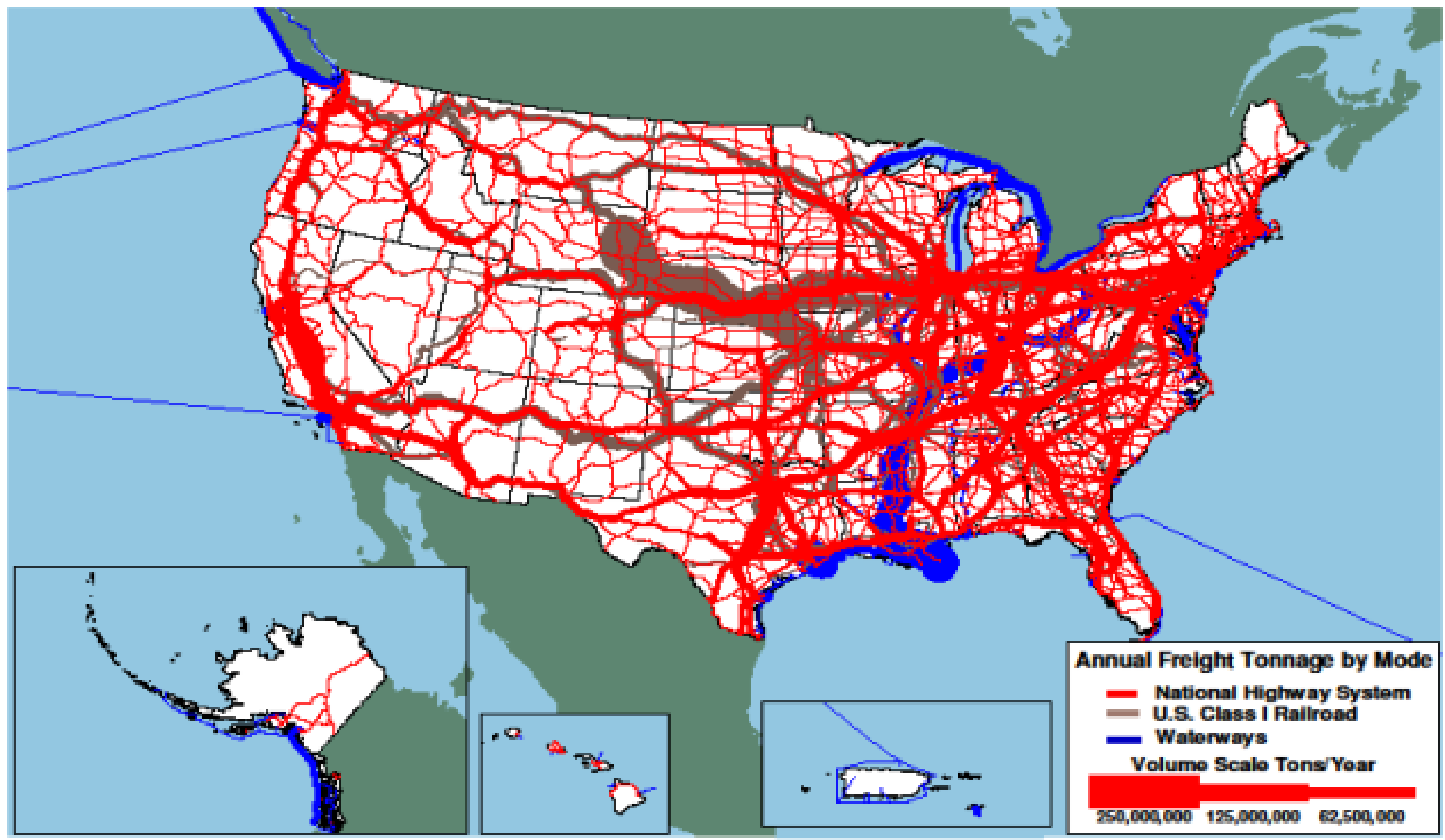
Sources: Highways-Federal Highway Administration, Freight Analysis Framework, Version 3.4, 2013; Rail-Surface Transportation Board, Annual Carload Waybill Sample, Federal Railroad Administration, rail freight flow assignments (2013); Waterways-U.S. Army Corps of Engineers (USACE), Annual Vessel Operating Activity, Tennessee Valley Authority, Lock Performance Monitoring System data for USACE, USACE Institute for Water Resources, Waterborne Foreign Trade Data, USACE water flow assignments (2013).
Freight Statistics
Many of the freight statistics in this section are derived from the Freight Analysis Framework (FAF) version 3 (FAF). FAF includes all freight flows to, from, and within the United States. FAF estimates are recalibrated every 5 years, primarily with data from the Commodity Flow Survey, and are updated annually with provisional estimates. The Commodity Flow Survey, conducted every 5 years by the Census Bureau and DOT's Bureau of Transportation Statistics, measures approximately two-thirds of the tonnage covered by the FAF. FAFincorporates data from the 2007 Commodity Flow Survey.
Statistics on trucking activity are primarily from FHWA's Highway Performance Monitoring System and the Census Bureau's Vehicle Inventory and Use Survey. This survey links truck size and weight, miles traveled, energy consumed, economic activity served, commodities carried, and other characteristics of significant public interest, but was discontinued after 2002. See www.ops.fhwa.dot.gov/freight/freight_analysis/faf for additional information. Efforts are underway to restart the Vehicle Inventory and Use Survey collection.
Freight movements are expected to increase over the next few decades as U.S. and global populations grow and consumer spending power increases both nationally and globally. More people and greater spending power will boost the production and consumption demand for many types of goods. All freight transportation modes are expected to experience increased volumes, although the amount of expected growth will vary from mode to mode, as Exhibit 1-20 shows.
Exhibit 1-18 Average Daily Long-Haul Freight Truck Traffic on the National Highway System, 20111
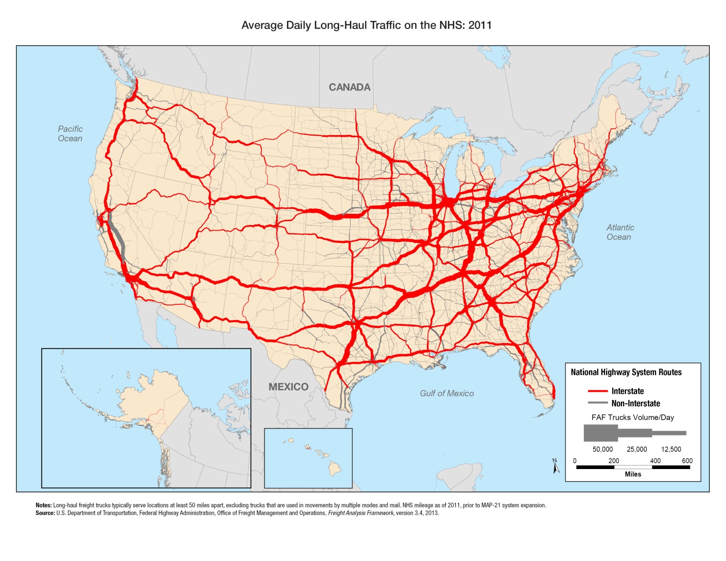
1Long-haul freight trucks typically serve locations at least 50 miles apart, excluding trucks that are used in movements by multiple modes and mail. NHS mileage as of 2011, prior to MAP-21 system expansion.
Sources: U.S. Department of Transportation, Federal Highway Administration, Office of Freight Management and Operations, Freight Analysis Framework, Version 3.4, 2013.
Exhibit 1-19 Annual Freight Transportation Services Index Values, 2000—2014 |
|
|---|---|
| Year |
Freight TSI1 |
| 2000 | 100 |
| 2005 | 112.4 |
| 2006 | 111.5 |
| 2007 | 110.1 |
| 2008 | 108.8 |
| 2009 | 98.3 |
| 2010 | 106.4 |
| 2011 | 110.8 |
| 2012 | 112.1 |
| 2013 | 116.2 |
| 2014 | 120.4 |
|
1 The TSI is indexed such that the Year 2000 TSI equals 100.0. Sources: U.S. Department of Transportation, Office of the Assistant Secretary for Research and Technology, Bureau of Transportation Statistics. |
|
Even though the annual volume increases are modest for all modes, the cumulative increase over 30 years for each mode is significant. This increased volume will strain the entire freight transportation network, most notably the highway network. Exhibit 1-21 displays a map of the 2040 truck tonnage information shown in Exhibit 1-20 plotted on the NHS.
Truck volume on many key truck routes of the NHS is expected to increase significantly between 2012 and 2040. These projected traffic increases would have major implications for highway congestion and freight movement efficiency, especially near large urban areas along or near major truck corridors.
Exhibit 1-20 Weight of Shipments by Transportation Mode1 |
||||
|---|---|---|---|---|
| Mode | Weight of Shipments (Millions of Tons) | Compound Annual Growth, 2010—2040 | ||
| 2007 | 2012 | 2040 Projected | ||
| Truck | 12,778 | 13,182 | 18,786 | 1.3% |
| Rail | 1,900 | 2,018 | 2,770 | 1.1% |
| Water | 950 | 975 | 1,070 | 0.3% |
| Air; Air and Truck | 13 | 15 | 53 | 4.6% |
| Multiple Modes and Mail2 | 1,429 | 1,588 | 3,575 | 2.9% |
| Pipeline | 1,493 | 1,546 | 1,740 | 0.4% |
| Other/Unknown | 316 | 338 | 526 | 1.6% |
| Total | 18,879 | 19,662 | 28,520 | 1.3% |
|
1 Data do not include imports and exports that pass through the United States from a foreign origin to a foreign destination by any mode. Numbers may not add to total due to rounding. 2 In this table, Multiple Modes and Mail includes export and import shipments that move domestically by a different mode than the mode used between the port and foreign location. Sources: U.S. Department of Transportation, Federal Highway Administration, Office of Freight Management and Operations, Freight Analysis Framework, version 3.4, 2014. |
||||
Exhibit 1-21 Average Daily Long-Haul Freight Truck Traffic on the National Highway System, 2040
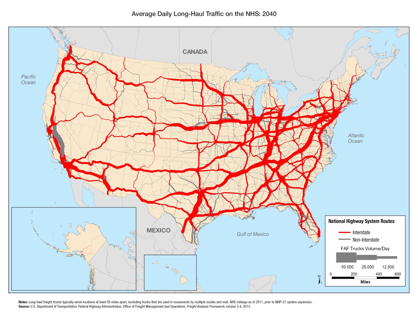
1Long-haul freight trucks typically serve locations at least 50 miles apart, excluding trucks that are used in movements by multiple modes and mail. NHS mileage as of 2011, prior to MAP-21 system expansion.
Sources: U.S. Department of Transportation, Federal Highway Administration, Office of Freight Management and Operations, Freight Analysis Framework, Version 3.4, 2013.
The differing freight volume and freight growth characteristics of the various freight transportation modes is related in large part to each mode's operating characteristics. These operating characteristics are key to determining how certain types of goods are transported. The routes, facilities, volumes, and service demands differ between higher-value, time-sensitive goods moving at high velocities and lower-value, cost-sensitive goods moving in bulk shipments, as shown in Exhibit 1-22.
Exhibit 1-22 The Spectrum of Freight Moved, 2007 |
||
|---|---|---|
| Parameter | Commodity Type | |
| High Value/Time Sensitive | Bulk | |
| Top Three Commodity Classes | Machinery | Gravel |
| Electronics | Cereal Grains | |
| Motorized Vehicles | Non-metallic mineral products | |
| Share of Total Tons | 13% | 65% |
| Share of Total Value | 58% | 16% |
| Key Performance Variables | Reliability | Reliability |
| Speed | Cost | |
| Flexibility | ||
| Share of Tons by Domestic Mode | 87% Truck | 71% Truck |
| 5% Multiple Modes and Mail | 12% Rail | |
| 4% Rail | 9% Pipeline | |
| 4% Multiple Modes and Mail | ||
| 3% Water | ||
| Share of Value by Domestic Mode | 70% Truck | 71% Truck |
| 16% Multiple Modes and Mail | 12% Pipeline | |
| 10% Air | 7% Multiple Modes and Mail | |
| 2% Rail | 6% Rail | |
| 2% Water | ||
| Sources: U.S. Department of Transportation, Federal Highway Administration and Bureau of Transportation Statistics, Freight Analysis Framework, version 3.6, 2015. | ||
Although trucking typically is considered a "faster" mode and handles a very high volume of high-value, time-sensitive goods, it also handles a significant share of lower-valued bulk tonnage. This share includes movement of agricultural products from farms, local distribution of gasoline, and pickup of municipal solid waste that cannot be handled readily by other transportation modes. The length of haul for activities such as these is typically very short.
Most trucking activity involves moving freight, and truck movements are a significant component of overall highway traffic. Three-fourths of vehicle miles traveled (VMT) by trucks larger than pickups and vans involves carrying freight, which encompasses a wide variety of products ranging from electronics to sand and gravel. Much of the rest of the large-truck VMT comprises empty backhauls of truck trailers or shipping containers. An increasing number of highways are carrying both a high volume and a high percentage of trucks. In 2011, for example, single-unit and combination trucks comprised more than 25 percent of the total average annual daily traffic on over 14,500 miles of NHS routes. On average, those routes accommodated at least 8,500 trucks per day.
Exhibit 1-23 presents a map identifying those major truck routes on the NHS, showing the routes that handle more than 8,500 trucks per day or experience daily traffic composed of at least 25 percent truck traffic.
Exhibit 1-23 Major Truck Routes on the National Highway System, 2011
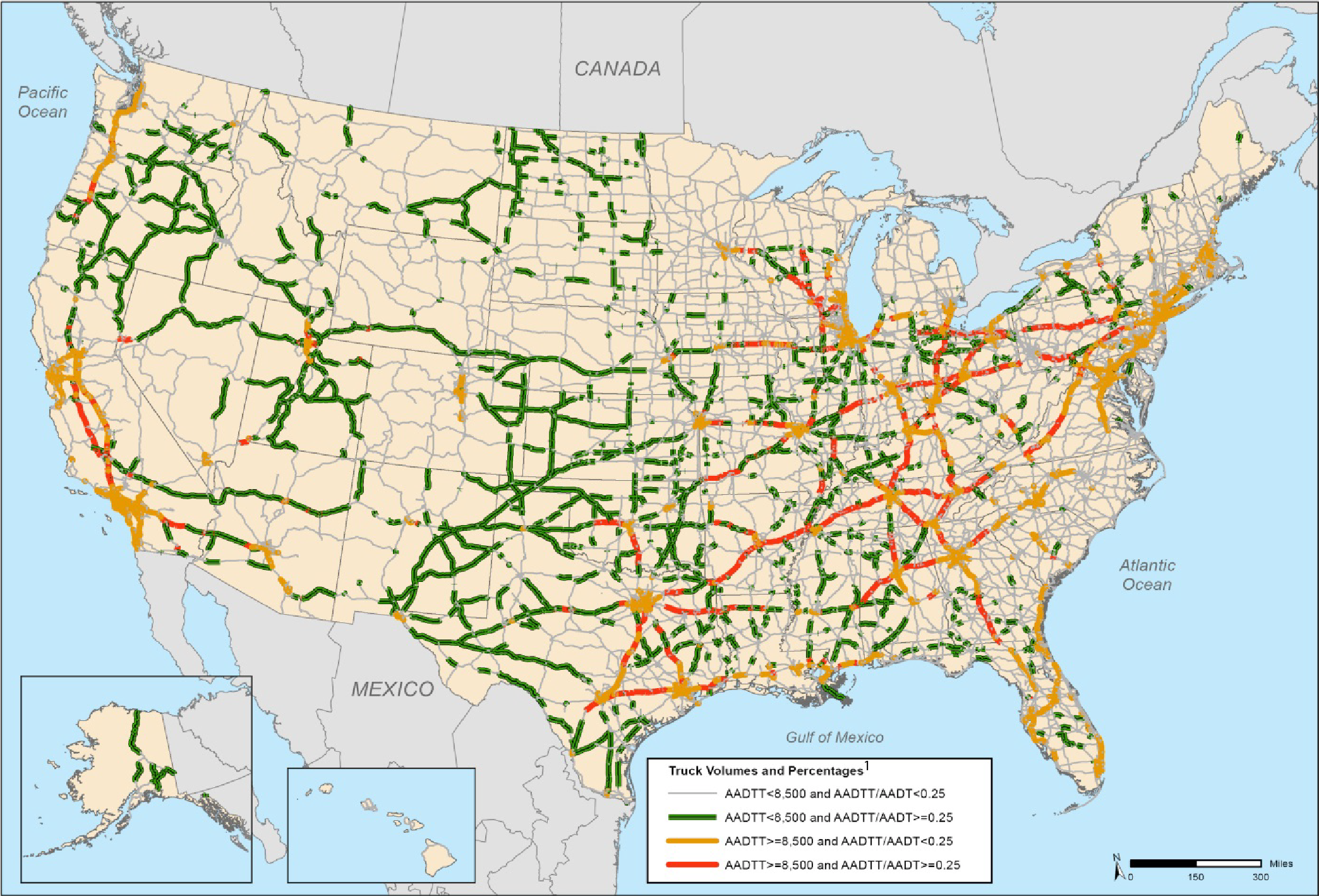
1AADTT is average annual daily truck traffic and includes all freight-hauling and other trucks with six or more tires. AADT is average annual daily traffic and includes all motor vehicles. NHS mileage as of 2011, prior to MAP-21 system expansion.
Sources: U.S. Department of Transportation, Federal Highway Administration, Office of Freight Management and Operations, Freight Analysis Framework, Version 3.4, 2013.
Although many freight movements are long-distance shipments to domestic or international locations, a larger percentage of shipments, particularly those by truck, are transported shorter distances. Approximately half of all trucks larger than pickups and vans operate locally-within 50 miles of home-and these short-haul trucks account for about 30 percent of truck VMT. By contrast, only 10 percent of trucks larger than pickups and vans operate more than 200 miles away from home, but these trucks account for more than 30 percent of truck VMT. Long-distance truck travel also accounts for nearly all freight ton miles and a large share of truck VMT. More information is shown in Exhibit 1-24.
Exhibit 1-24 Trucks and Truck Miles by Range of Operations1 |
||
|---|---|---|
| Location | Number of Trucks (percent) | Truck Miles (percent) |
| Off the Road | 3.3% | 1.6% |
| 50 Miles or Less | 53.3% | 29.3% |
| 51 to 100 Miles | 12.4% | 13.2% |
| 101 to 200 Miles | 4.4% | 8.1% |
| 201 to 500 Miles | 4.2% | 12.1% |
| 501 Miles or More | 5.3% | 18.4% |
| Not Reported | 13.0% | 17.3% |
| Not Applicable | 4.1% | 0.1% |
| Total | 100% | 100% |
|
1 Includes trucks registered to companies and individuals in the United States except pickups, minivans, other light vans, and sport utility vehicles. Numbers may not add to total due to rounding. Sources: U.S. Department of Commerce, Census Bureau, 2002 Vehicle Inventory and Use Survey: United States, EC02TV-US, Table 3a (Washington, DC: 2004), available at http://www.census.gov/prod/ec02/ec02tv-us.pdf as of March 13, 2015. |
||
Many U.S. freight movements are part of international trade between the United States and other countries. Canada and Mexico, which according to the U.S. Census Bureau are the United States' largest and third-largest trading partners, respectively, account for a significant portion of these international freight movements, including all freight movements on land surface modes. Exhibits 1-25 and 1-26 show U.S.-Canada trade volumes by value and tonnage, respectively, for trucks, railroads, and all modes combined (including non-land surface modes).
Exhibits 1-27 and 1-28 show U.S.-Mexico trade volumes by value and tonnage, respectively, for trucks, railroads, and all modes combined (including nonland surface modes).
Exhibit 1-25 Total U.S.-Canada Trade Value by Transportation Mode, 2000—20141 |
Exhibit 1-26 Total U.S.-Canada Trade Tonnage by Transportation Mode, 2000—2013 |
|||||||
|---|---|---|---|---|---|---|---|---|
| Year | Total Trade Value (Millions of U.S. Dollars) | Year | Total Trade Tonnage (Thousands of Metric Tons) | |||||
| Truck | Rail | All Modes | Truck | Rail | All Modes | |||
| 2000 | $257,642 | $62,646 | $409,779 | 2000 | N/A | N/A | 364,230.00 | |
| 2005 | $294,917 | $79,928 | $499,291 | 2005 | 133,679.40 | 98,775.90 | 414,328.40 | |
| 2006 | $314,202 | $85,736 | $533,673 | 2006 | 130,752.80 | 102,453.70 | 420,589.40 | |
| 2007 | $324,747 | $91,459 | $561,548 | 2007 | 116,995.90 | 105,099.80 | 414,405.50 | |
| 2008 | $319,946 | $93,194 | $596,470 | 2008 | 110,337.00 | 98,011.60 | 406,014.30 | |
| 2009 | $247,757 | $61,032 | $429,587 | 2009 | 92,542.00 | 72,107.00 | 333,343.30 | |
| 2010 | $299,886 | $82,999 | $526,893 | 2010 | 104,138.60 | 87,933.70 | 371,862.20 | |
| 2011 | $334,012 | $94,797 | $596,616 | 2011 | 106,410.30 | 91,875.90 | 387,757.20 | |
| 2012 | $344,919 | $103,050 | $616,913 | 2012 | 107,216.10 | 97,625.80 | 409,211.30 | |
| 2013 | $348,332 | $105,409 | $634,162 | 2013 | 108,764.80 | 104,701.30 | 426,797.60 | |
| 2014 | $353,955 | $104,155 | $658,188 | |||||
|
1The monetary values shown are not adjusted for inflation. Sources: U.S. Department of Transportation, Bureau of Transportation Statistics, North American Transborder Freight Data, available at www.bts.gov/transborder as of April 10, 2015. |
Sources: U.S. Department of Transportation, Bureau of Transportation Statistics, North American Transborder Freight Data, available at www.bts.gov/transborder as of April 10, 2015. |
|||||||
Exhibit 1-27 Total U.S.-Mexico Trade Value by Transportation Mode, 2000—20141 |
Exhibit 1-28 Total U.S.-Mexico Trade Tonnage by Transportation Mode, 2000—2013 |
|||||||
|---|---|---|---|---|---|---|---|---|
| Year | Total Trade Value (Millions of U.S. Dollars) | Year | Total Trade Tonnage (Thousands of Metric Tons) | |||||
| Truck | Rail | All Modes | Truck | Rail | All Modes | |||
| 2000 | $171,058 | $31,552 | $247,275 | 2000 | N/A | N/A | 161,888.00 | |
| 2005 | $195,609 | $36,530 | $290,247 | 2005 | 47,630.90 | 17,369.00 | 190,116.20 | |
| 2006 | $219,455 | $43,135 | $332,426 | 2006 | 49,254.90 | 17,879.40 | 195,741.40 | |
| 2007 | $230,084 | $46,400 | $347,340 | 2007 | 56,918.80 | 35,060.10 | 212,331.70 | |
| 2008 | $234,488 | $47,230 | $367,453 | 2008 | 54,944.10 | 35,801.30 | 200,337.10 | |
| 2009 | $207,195 | $34,591 | $305,525 | 2009 | 48,254.60 | 26,251.60 | 172,558.20 | |
| 2010 | $260,331 | $48,144 | $393,650 | 2010 | 65,703.40 | 33,762.30 | 214,598.30 | |
| 2011 | $295,522 | $57,270 | $461,162 | 2011 | 82,115.70 | 36,980.50 | 242,456.30 | |
| 2012 | $323,170 | $64,399 | $493,500 | 2012 | 70,736.10 | 41,889.00 | 228,823.70 | |
| 2013 | $335,351 | $69,851 | $506,608 | 2013 | 69,426.30 | 38,446.90 | 222,606.10 | |
| 2014 | $360,668 | $73,690 | $534,484 |
1 The monetary values shown are not adjusted for inflation. Sources: U.S. Department of Transportation, Bureau of Transportation Statistics, North American Transborder Freight Data, available at www.bts.gov/transborder as of April 10, 2015. |
Sources: U.S. Department of Transportation, Bureau of Transportation Statistics, North American Transborder Freight Data, available at www.bts.gov/transborder as of April 10, 2015. |
|||
Freight Challenges
The challenges of moving the Nation's freight cheaply and reliably on an increasingly constrained infrastructure without affecting safety or degrading the environment are substantial, and traditional strategies to support passenger travel might not apply. The freight transportation challenge differs from that of urban commuting and other passenger travel in several ways:
- Freight often moves long distances through localities and responds to distant economic demands, while most passenger travel occurs locally. Freight movement often creates local problems without local benefits. Local residents and elected officials are also less likely to have direct experience in freight transportation operations, making it more difficult for such improvements to be seen as a priority.
- Freight movement fluctuates more, and more quickly, than passenger travel does. Although both passenger travel and freight respond to long-term demographic changes, freight responds more quickly than passenger travel to short-term economic fluctuations. Fluctuations can be national or local. The addition or loss of even a single major business can dramatically change the level of freight activity in a locality.
- Freight movement is heterogeneous compared with passenger travel. Patterns of passenger travel tend to be similar across metropolitan areas and among large economic and social strata. Freight transportation demands differ radically in terms of the types of freight vehicles used and the locations they serve. For example, farms, mines, manufacturing plants, commercial retail shopping centers, grocery stores, and online retail sales all have significantly different locations, shipment frequencies, and general shipment needs. These differences occur not only between freight transportation modes but also within freight transportation modes. As one example, the operating characteristics of long-haul tractor-trailers serving one location per shipment load distinctly differ from those of shorter-haul tractor-trailers and large single-unit trucks serving multiple locations per shipment load. Both are distinctly different from parcel carriers that use smaller, single-unit trucks and serve many locations per shipment load. Solutions aimed at "average" conditions are less likely to succeed because the freight demands of economic sectors vary widely.
- To the extent that freight movement is concentrated in different corridors or locations than passenger travel, transportation system investments targeted solely at improving general traffic conditions may be less likely to specifically aid the flow of freight.
- The reliable movement of freight depends on all modes working together such that the multimodal freight system functions smoothly and without costly delays. Bottlenecks on one mode of transportation can affect the performance of freight throughout the network.
Local public action to support the economic benefits of freight transportation is difficult to marshal because freight traffic and the benefits of serving that traffic rarely stay within a single political jurisdiction. One-half the weight and two-thirds the value of all freight movements cross a State or international boundary. Additionally, locations desirable from a developer's standpoint for industrial and commercial development are often highly sensitive to non-transportation considerations such as local zoning, tax rates, and development incentives. Such considerations can pit adjacent municipalities or counties against one another and undermine comprehensive freight transportation planning efforts. Federal legislation established metropolitan planning organizations in the 1960s to coordinate transportation planning and investment across State and local lines within urban areas. Both the interregional nature of many freight movements and the varying levels of support or opposition in local jurisdictions for freight-generating development, however, complicate the metropolitan area transportation planning process. Creative and ad hoc arrangements often are required through pooled-fund studies and multi-State coalitions to plan and invest in freight corridors that span regions and even the continent, but few institutional arrangements coordinate this activity. One example of a more established multi-State arrangement is the I-95 Corridor Coalition. Additional information about this coalition and similar groups can be found at www.ops.fhwa.dot.gov/freight/corridor_coal.htm.
The growing needs of freight transportation can bring into focus conflicts between national, State, and local interests. Many longer-haul truck, train, and other freight movements create negative impacts, such as increased noise and dirt, and provide only limited benefits to localities. Those transits, however, can greatly influence national freight movement and regional economies.
Beyond the challenges of intergovernmental coordination, freight transportation raises additional issues involving the relationships between public and private sectors. Virtually all carriers and many freight facilities are privately owned. Freight Facts and Figures 2015 shows that the private sector owns $1.173 trillion in transportation equipment plus $739 billion in transportation structures. In comparison, public agencies own $686 billion in transportation equipment and $3.343 trillion in highways. The private sector owns virtually all freight railroad facilities and services, and trucks owned by the private sector operate over public highways. Likewise, air cargo services that the private sector owns operate in public airways and primarily at public airports.
Challenges for Freight Transportation: Congestion
Congestion affects economic productivity in several ways. American businesses require more operators and equipment to deliver goods when shipping takes longer, more inventory when deliveries are unreliable or disrupted in some way, and more distribution centers to reach markets quickly when traffic is slow. Likewise, sluggish traffic on the ground and in the air affects both businesses and households, reducing the number of workers and job sites within easy reach of any location. The growth in freight is a major contributor to congestion in urban areas and on intercity routes, and congestion affects the timeliness and reliability of freight transportation. Long-distance freight movements are often a significant contributor to local congestion, and local congestion typically impedes freight to the detriment of local and distant economic activity.
Growing freight demand increases recurring congestion at freight bottlenecks, places where freight and passenger service conflict with one another, and where room for local pickup and delivery is insufficient. Congested freight hubs include international gateways such as water ports, airports, and border crossings, and major domestic terminals and transfer points such as distribution center hubs in large metropolitan areas and rail yards in major railroad centers such as Chicago, Kansas City, and Dallas/Fort Worth. In many cases, inadequate connections between a freight hub and the nearby highway network create congestion chokepoints. Bottlenecks on intercity corridors between freight hubs are caused by converging traffic at highway intersections and railroad junctions, steep grades on highways and rail lines, lane reductions on highways and single-track portions of railroads, and locks and constrained channels on waterways.
Congestion also is caused by restrictions on freight movement, such as the lack of space for trucks in dense urban areas and limited delivery and pickup times at ports, terminals, and shipper loading docks. The Off-Hours Delivery Project in New York City found that, for a large percentage of urban deliveries (between 40 percent and 78 percent ), receivers-the stores and businesses receiving freight shipments-decide when the deliveries are made. The result is that many freight deliveries cannot be shifted readily to lower congestion times.The same study also determined, however, that freight deliveries made during off-hour periods were 30 percent cheaper than deliveries during regular business hours.Limitations on delivery times place significant demands on highway rest areas when large numbers of trucks park outside major metropolitan areas waiting for their destination to open and accept their shipments. The Jason's Law Truck Parking Study mandated in MAP-21 was completed in August 2015 by FHWA, and it examined truck-parking needs throughout the United States. The study highlighted the need for additional truck parking facilities and recommended incorporating truck parking analyses into freight planning at the State and regional level, as well as increased regional coordination by Freight Stakeholder Advisory Groups.
Bottlenecks cause recurring, predictable congestion in various locations having high transportation volume. Additionally, less predictable, nonrecurring congestion can also create challenges for freight movements across all modes, especially those that are time sensitive. Sources of nonrecurring delay include incidents, weather, work zones, and other disruptions. In some cases, disruptions not only cause nonrecurring congestion, but also cause freight diversions. According to the Port of New York-New Jersey, Superstorm Sandy forced a diversion of 57 ships, 9,000 vehicles, and 15,000 shipping containers from the port to other East Coast ports.The Port of Hampton Roads in southeastern Virginia alone handled more than 8,000 of the diverted containers.The Virginia Port Authority, trucking companies, CSX, Norfolk Southern, and U.S. Customs and Border Protection all needed to coordinate to handle the unexpected volume of shipments and ensure the shipments were transported to the proper locations.
Chapter 5 includes a broader discussion of system performance, including congestion's impacts on system performance.
1U.S. Department of Transportation, Integrative Freight Demand Management in the New York City Metropolitan Area, September 30, 2010, page 27 http://transp.rpi.edu/~usdotp/OHD_FINAL_REPORT.pdf.
2U.S. Department of Transportation, Integrative Freight Demand Management in the New York City Metropolitan Area, September 30, 2010, pages 6—7 http://transp.rpi.edu/~usdotp/OHD_FINAL_REPORT.pdf.
3Southworth, F., et al. NCFRP Report 30, Making U.S. Ports Resilient as Part of Extended Intermodal Supply Chains, Transportation Research Board, 2014, page 50 http://onlinepubs.trb.org/onlinepubs/ncfrp/ncfrp_rpt_030.pdf.
4Southworth, F., et al. NCFRP Report 30, Making U.S. Ports Resilient as Part of Extended Intermodal Supply Chains, Transportation Research Board, 2014, page 52 http://onlinepubs.trb.org/onlinepubs/ncfrp/ncfrp_rpt_030.pdf.
Challenges for Freight Transportation: Safety, Energy, and the Environment
Freight transportation is not simply an issue of throughput and congestion. The growth in freight movement has heightened public concerns about safety, energy consumption, and the environment.
Highways and railroads account for nearly all fatalities and injuries involving freight transportation. Most of these fatalities involve people who are not part of the freight transportation industry, such as trespassers at railroad facilities and occupants of other vehicles killed in crashes involving large trucks. The BTS Freight Facts and Figures 2015 shows that, of the 32,719 highway fatalities in 2013, 2.1 percent were occupants of large trucks and 10.0 percent were others killed in crashes involving large trucks (the remaining 87.9 percent of fatalities were attributed to other types of personal and commercial vehicles). Chapter 5 of Freight Facts and Figures 2015discusses highway safety in more detail.
According to Freight Facts and Figures 2015, single-unit and combination trucks accounted for 25.5 percent of all gasoline, diesel, and other fuels consumed by motor vehicles in 2013. Fuel consumption by trucks resulted in 78 percent of the 388.3 million metric tons of carbon dioxide equivalent generated by freight transportation, and freight accounted for 21.9 percent of transportation's contribution to the emissions of this major greenhouse gas. Trucks and other heavy vehicles that operate on the U.S. highway system are also a major contributor to air quality problems related to nitrogen oxide and PM-10 (particulate matter 10 microns in diameter or smaller). Absolute freight truck-related emissions, however, have declined significantly with the increased use of ultralow-sulfur diesel; nitrogen oxide emissions from freight trucks fell 44.6 percent between 2005 and 2012, and PM-10 emissions declined 44.8 percent during the same period.
Environmental issues involving freight transportation go well beyond emissions. Disposal of dredge spoil-the mud and silt that must be removed to deepen water channels for commercial vessels-is a major challenge associated with allowing larger ships to berth. Land use and water quality concerns due to various factors such as soil contamination are raised against all types of freight facilities, and invasive species can spread through freight movement.
Incidents involving hazardous materials exacerbate public concern and cause serious disruption.Freight Facts and Figures 2015 shows that, of the 15,433 transportation incidents in 2012 involving hazardous materials, highways accounted for 13,241 accidents (85.8 percent of hazardous material transportation incidents), air accounted for 1,293 accidents (9.5 percent of incidents), rail accounted for 662 accidents (4.3 percent of incidents), and water accounted for 70 accidents (0.5 percent of incidents). The railcar fire in the Howard Street tunnel in the city of Baltimore in 2001 illustrates both the perceived and real problems of transporting hazardous materials. This incident, which occurred on tracks near a major league baseball stadium at game time during the evening rush hour, forced the evacuation of thousands of people and closed businesses in much of downtown Baltimore. A vital railroad link between the Northeast and the South and a local rail transit line and all east-west arterial streets through downtown were closed for an extended period. More recent hazardous material incidents, such as the multiple petroleum-shipping train derailments that have occurred in different parts of the country, although not as widely disruptive to the U.S. transportation system as the 2001 Baltimore accident was, also have created significant short-term disruptions on freight transportation movements, negative environmental impacts, and in extreme cases, human fatalities.
Privately owned ships operate over public waterways and at both public and private port facilities. Most pipelines are privately owned but are significantly controlled by public regulation. In the public sector, State or local governments own virtually all truck routes, and regional or local authorities typically own airports and harbors. Air and water navigation is typically handled at the Federal level, and safety is regulated by all levels of government. Because of this mixed ownership and management, most solutions to freight problems require coordinated action by a wide variety of public and private-sector organizations and companies. Financial, planning, and other institutional mechanisms for developing and implementing joint efforts have been limited, inhibiting effective measures to improve the performance and minimize the public costs of the freight transportation system.
Freight challenges are not new. Their ongoing importance and increased complexity, however, warrant creative solutions by all parties having a stake in the vitality of the American economy.
National Freight Policy
The 2012 passage of the Moving Ahead for Progress in the 21st Century (MAP-21) transportation reauthorization created a formal U.S. policy to improve the condition and performance of the national freight network. This network is critical for ensuring the United States remains competitive in the global economy and achieves various goals to improve the Nation's freight movement (Section 1115). MAP-21 has greatly increased the visibility and emphasis on freight transportation at the Federal level. MAP-21 required the designation of a primary freight network and creation of a national freight strategic plan, a freight conditions and performance report, and new or refined transportation investment and planning tools to evaluate freight-related and non-freight related projects. All these provisions, and others in MAP-21, such as prioritizing projects to improve freight movement (Section 1116), encouraging States to establish freight advisory committees (Section 1117), encouraging States to develop State freight plans (Section 1118), and requiring creation of freight performance measures and performance targets that the States will use to assess freight movement on the Interstate system (Section 1203), have increased the focus on addressing and improving freight transportation at the Federal, State, and regional/metropolitan level. Many States and metropolitan planning organizations were already engaged in formal or informal freight transportation planning efforts before MAP-21 was passed. The current reauthorization has helped formalize these efforts, however, both in States and metropolitan planning organizations that have already been actively engaged in freight planning and where freight planning efforts have been limited, irregular, or nonexistent.
MAP-21 also indirectly encouraged other initiatives intended to promote better understanding of freight activities and to address freight challenges at all levels of government and in the private sector. DOT has created a Freight Policy Council involving the Office of the Secretary and all of DOT's freight-related modal administrations to coordinate the implementation of MAP-21 freight provisions, including the National Freight Strategic Plan and the National Freight Network. DOT also created a National Freight Advisory Committee composed of various public and private-sector representatives to provide advice and recommendations to the DOT Secretary on many of the MAP-21 freight-related provisions.
The Fixing America's Surface Transportation (FAST) Act established a national policy of maintaining and improving the condition and performance of the National Highway Freight Network (i.e., Network) to identify the highest priority highway freight routes and ensure these routes are appropriately improved and maintained to enhance the United States' ability to compete in the global economy. The FAST Act established a national highway freight program and specified goals associated with this national policy. Those goals include investing in infrastructure improvements and improving the safety, security, efficiency, productivity, resiliency, and reliability of the Network. The FAST Act requires DOT to develop a National Freight Strategic Plan that identifies and assesses the conditions of the Network and forecasts its future needs. It also required DOT to establish a National Multimodal Freight Network that will assist in strategically directing resources toward improved system performance and the prioritization of Federal investments.
-
Blumenberg, Evelyn, Moving In and Moving Around: Immigrants, Travel Behavior, and Implications for Transport Policy, Institute of Transportation Studies, UCLA School of Public Affairs, 2008. ↑
-
Holguin-Veras, J., K. Ozbat, and A.de Cerreño. Evaluation Study of Port Authority of New York and New Jersey's Time of Day Pricing. March 2005. NJ Department of Transportation. FHWA/NJ-2005-005. ↑
-
Multisystems, Inc. Fare Policies, Structures, and Technologies: Update. 2003. TCRP Report 94. http://onlinepubs.trb.org/onlinepubs/tcrp/tcrp_rpt_94.pdf. ↑
-
This standard defines the data format used on Proximity Integrated Circuit Cards (PICC). This part provides a consistent and uniform method for storing, retrieving, and updating data from contactless fare media used in transit applications. It also references related international standards that define the physical, electrical, and communications aspects of PICCs. Source: APTA. "Universal Transit Fare System Task Force." APTA Standards Development Program Website. Available at: http://www.aptastandards.com/StandardsPrograms/UTFSStandards/TaskForce/tabid/82/language/en-US/Default.aspx, as of 27 July 2011. ↑
-
Geron, T. Airbnb and the Unstoppable Rise of the Share Economy. Forbes. January 23, 2013. ↑
-
The rise of the sharing economy, http://www.economist.com/news/leaders/21573104-internet-everything-hire-rise-sharing-economy, March 9, 2013. ↑
-
California, Assembly Bill 1871, 2011. ↑
-
Martin, E.W., and S. Shaheen, Greenhouse Gas Emissions Impacts of Carsharing in North America, Mineta Transportation Institute, 2011. ↑
-
Boarnet, M.G., S. Handy, and K. Lovejoy, Impacts of Carsharing on Passenger Vehicle Use and Greenhouse Gas Emissions, California Air Resources Board, 2013. ↑
-
Martin, E.W., and S. Shaheen, Greenhouse Gas Emissions Impacts of Carsharing in North America, Mineta Transportation Institute, 2011. ↑
-
U.S. Census Bureau, Journey to Work, 2010 ↑
-
Commuting in America 2013: The National Report on Commuting Patterns and Trends, Brief 6. Job Dynamics, AASHTO, January 2015 ↑
-
Commuting in America 2013: The National Report on Commuting Patterns and Trends, Brief 6. Job Dynamics, AASHTO, January 2015, pg. 5. ↑
-
http://www.cleanaircampaign.org/About-Us. ↑
-
Sylvia Y. He, Lingqian Hu, Telecommuting, Income and Out-of-home Activities, Travel Behaviour and Society, 2015 ↑