Chapter 7: Potential Capital Investment Impacts - 2015 Conditions and Performance - Policy

The analyses presented in this section use a common set of assumptions to derive relationships between alternative levels of future highway capital investment and various measures of future highway and bridge conditions and performance. A subsequent section in this chapter provides comparable information for different types and levels of potential future transit investments.

This section examines the types of investment within the scopes of the Highway Economic Requirements System (HERS) and the National Bridge Investment Analysis System (NBIAS) and lays the foundation for the capital investment scenarios for highways presented in Chapter 8. The accuracy of the projections for highway investments in this chapter depends on the validity of the technical assumptions underlying the analysis, some of which are explored in the sensitivity analysis in Chapter 10. The analyses presented in this section make no explicit assumptions regarding how future investment in highways might be funded.

Types of Capital Spending Projected by HERS and NBIAS

The types of investments HERS and NBIAS evaluate can be related to the system of highway functional classification introduced in Chapter 2 and to the broad categories of capital improvements introduced in Chapter 6 (system rehabilitation, system expansion, and system enhancement). NBIAS relies on the National Bridge Inventory (NBI) database, which covers bridges on all highway functional classes, and evaluates improvements that generally fall within the system rehabilitation category.

HERS evaluates pavement improvements-resurfacing or reconstruction-and highway widening; the types of improvements included in these categories roughly correspond to system rehabilitation and system expansion as described in Chapter 6. In estimating the per-mile costs of widening improvements, HERS recognizes a typical number of bridges and other structures that would need modification. Thus, the estimates from HERS are considered to represent system expansion costs for both highways and bridges. Coverage of the HERS analysis is limited, however, to Federal-aid highways, as the Highway Performance Monitoring System (HPMS) sample does not include data for rural minor collectors, rural local roads, or urban local roads.

The term "nonmodeled spending" refers in this report to spending on highway and bridge capital improvements that are not evaluated in HERS or NBIAS; such spending is not included in the analyses presented in this chapter, but the capital investment scenarios presented in Chapter 8 are adjusted to account for them. Nonmodeled spending includes capital improvements on highway classes omitted from the HPMS sample and hence the HERS model. The development of the future investment scenarios for the highway system as a whole thus required supplementary estimation outside the HERS modeling process.

Nonmodeled spending also includes types of capital expenditures classified in Chapter 6 as system enhancements, which neither HERS nor NBIAS currently evaluate. Although HERS incorporates assumptions about future operations investments, the capital components of which would be classified as system enhancements, the model does not directly evaluate the need for these deployments. In addition, HERS does not identify specific safety-oriented investment opportunities, but instead considers the ancillary safety impacts of capital investments that are directed primarily toward system rehabilitation or capacity expansion. This limitation of the model owes to the HPMS database's containing no information on the locations of crashes and safety devices such as guardrails or rumble strips.

How closely do the types of capital improvements modeled in HERS and NBIAS correspond to the specific capital improvement type categories presented in Chapter 6?

Exhibit 6-12 (see Chapter 6) provides a crosswalk between a series of specific capital improvement types for which data are routinely collected from the States and three major summary categories: system rehabilitation, system expansion, and system enhancement. The types of improvements covered by HERS and NBIAS are assumed to correspond with the system rehabilitation and system expansion categories. As in Exhibit 6-12, HERS splits spending on "reconstruction with added capacity" among these categories.

For some of the detailed categories in Exhibit 6-12, the assumed correspondence is close overall but not exact. In particular, the extent to which HERS covers construction of new roads and bridges is ambiguous. Although not directly modeled in HERS, such investments are often motivated by a desire to alleviate congestion on existing facilities in a corridor, and thus would be captured indirectly by the HERS analysis in the form of additional normal-cost or high-cost lanes. As described in Appendix A, the costs per mile assumed in HERS for high-cost lanes are based on typical costs of tunneling, double-decking, or building parallel routes, depending on the functional class and area population size for the section being analyzed. To the extent that investments in the "new construction" and "new bridge" improvement types identified in Chapter 6 are motivated by desires to encourage economic development or accomplish other goals aside from the reduction of congestion on the existing highway network, such investments would not be captured in the HERS analysis.

Some other comparability issues include:

Some of the relocation expenditures identified in Exhibit 6-12 could be motivated by considerations beyond those reflected in the curve and grade rating data that HERS uses in computing the benefits of horizontal and vertical realignments.
The bridge expenditures that Exhibit 6-12 counts as system rehabilitation could include work on bridge approaches and ancillary improvements that NBIAS does not model.
HERS and NBIAS are assumed not to capture improvements that count as system enhancement spending, including the spending on the "safety" category in Exhibit 6-12. Some safety deficiencies, however, might be addressed as part of broader pavement and capacity improvements modeled in HERS.
The HERS operations preprocessor described in Appendix A includes capital investments in operations equipment and technology that would fall under the definition of the "traffic management/engineering" improvement type in Chapter 6. These investments are counted among the nonmodeled system enhancements because they are not evaluated within the benefit-cost framework that HERS applies to system preservation and expansion investments.

Exhibit 7-1 shows that, systemwide in 2012, highway capital spending was $105.2 billion, of which $57.4 billion was for the types of improvement that HERS models and $16.4 billion was for the types of improvement NBIAS models. The other $31.4 billion, which was for nonmodeled highway capital spending, was divided about evenly between system enhancement expenditures and capital improvements to classes of highways not reported in HPMS.

Exhibit 7-1 Distribution of 2012 Capital Expenditures by Investment Type

A set of four pie charts shows the distribution of capital expenditures in billions of dollars by investment type. For interstate system expenditures, which amount to $20.5 billion total, improvement types modeled in HERS account for $15.2 billion or 74.0 percent ; improvement types modeled in NBIAS account for $3.8 billion or 18.7 percent ; and improvement types not modeled in HERS or NBIAS account for $1.5 billion or 7.3 percent . For National Highway System expenditures, which amount to $54.6 billion total, improvement types modeled in HERS account for $40.8 billion or 74.7 percent ; improvement types modeled in NBIAS account for $8.3 billion or 15.3 percent ; and improvement types not modeled in HERS or NBIAS account for $5.5 billion or 10.0 percent . For Federal-aid highways expenditures, which amount to $79.0 billion total, improvement types modeled in HERS account for $57.4 billion or 72.7 percent ; improvement types modeled in NBIAS account for $12.0 billion or 15.2 percent ; and improvement types not modeled in HERS or NBIAS account for $9.6 billion or 12.1 percent . For system-wide (all roads) expenditures, which amount to $105.2 billion total, improvement types modeled in HERS account for $57.4 billion or 54.5 percent ; improvement types modeled in NBIAS account for $16.4 billion or 15.6 percent ; improvement types not modeled in HERS or NBIAS account for $15.9 billion or 15.1 percent ; and highway functional systems not reported in HPMS account for $15.5 billion or 14.8 percent . Source: Highway Statistics 2012 (Table SF-12A) and unpublished FHWA data.

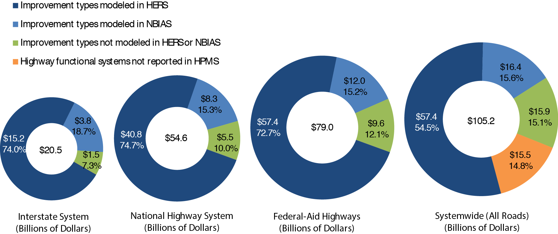
Source: Highway Statistics 2012 (Table SF-12A) and unpublished FHWA data.

Because the HPMS sample data are available only for Federal-aid highways, the percentage of capital improvements classified as nonmodeled spending is lower for Federal-aid highways than is the case systemwide. Of the $79.0 billion spent by all levels of government on capital improvements to Federal-aid highways in 2012, 72.7 percent was within the scope of HERS, 15.2 percent was within the scope of NBIAS, and 12.1 percent was for spending captured by neither. The percentage distribution differs somewhat for the Interstate System, with a slightly higher share within the scope of HERS and NBIAS (74.0 percent and 18.7 percent , respectively) and a smaller share captured by neither (7.3 percent ).

Of note is that the statistics presented in this chapter and in Chapter 8 relating to future National Highway System (NHS) investment are based on an estimate of how the NHS will look after its expansion pursuant to MAP-21, rather than as the system existed in 2012. Although the 2012 HPMS sample data incorporate the MAP-21-driven expansion of the NHS, the 2012 NBI data do not reflect the expanded NHS. As indicated in Chapter 6, combined highway capital spending by all levels of government on the NHS in 2012 totaled $44.6 billion. The NHS capital spending figure of $54.6 billion referenced in Exhibit 7-1 includes amounts spent on other principal arterials, as much of this mileage was be added to the NHS by MAP-21.

Treatment of Traffic Growth

For the HERS analysis in this report, growth in vehicle miles traveled (VMT) is based on two primary inputs: HPMS section-level forecasts of future annual average daily traffic that States provide and a national-level forecast developed from a new FHWA model. The national-level forecast serves as a control, which the sum of the forecast section-level changes in VMT must match. To match the national-level control, the section-level forecasts are scaled proportionally. For this report, the sum of the section-level forecasts yielded an aggregate average annual VMT growth rate of 1.42 percent that exceeded the national-level forecast of 1.04 percent per year, and thus were scaled proportionally downward to match the national-level forecast. Chapter 9 discusses the national-level forecast and reviews the accuracy of VMT projections in previous C&P Reports.

The national-level forecast includes separate VMT growth rates for light-duty vehicles, single-unit trucks, and combination trucks; these separate growth rates were applied in the HERS analysis. VMT in light-duty vehicles is forecast to grow at 0.92 percent per year. VMT for heavy-duty vehicles is forecast to grow at a rate more than twice that for light-duty vehicles (2.15 percent per year for single-unit trucks and 2.12 percent per year for combination trucks). The higher rate of forecast VMT growth for heavy-duty vehicles reflects a close relationship between heavy-vehicle VMT and economic output (GDP or gross domestic product). Economic factors (e.g., sensitivity of VMT demand to income and fuel prices) also influence the forecast of light-duty VMT, but to a weaker extent than the influence on heavy-duty vehicles. The difference in projected VMT growth rates for heavy-duty and light-duty vehicles reflects the direct role of freight transportation in facilitating the production and sale of outputs measured within GDP; increases in income associated with GDP growth do not influence light-duty VMT to the same degree.

The procedures used for estimating traffic growth in the NBIAS analysis presented in this report are similar to those used for HERS. For NBIAS, these forecasts build off bridge-level forecasts of future average daily traffic that States provide in the NBI. The sum of the bridge-level forecasts yielded an aggregate growth rate of 1.46 percent per year; growth rates for individual bridges were adjusted downward to match the 1.04 percent control total from the national-level VMT forecast model referenced above. Unlike the HERS analysis, the NBIAS analysis applied the same growth rate to all vehicle classes, as NBIAS is not currently equipped to handle separate growth rates by vehicle type.

An underlying assumption applied in both HERS and NBIAS is that VMT will grow linearly (so that 1/20th of the additional VMT is added each year), rather than geometrically (i.e., at a constant annual rate). With linear growth, the annual rate of growth gradually declines over the forecast period. Estimated VMT growth rates within each highway investment scenario deviate from the FHWA forecast values due to estimated changes in user travel cost, as discussed in the following section.

In previous reports, the State-reported travel growth forecasts in the HPMS and the NBI were applied directly (i.e., they were not scaled to match a national-level control). Chapter 10 considers an alternative in which VMT grows consistently with the State-reported forecasts.

Alternative Levels of Future Capital Investment Analyzed

Both the HERS and NBIAS analyses presented in this chapter assume that capital investment within the scopes of the models will grow over 20 years at a constant annual percentage rate, which could be positive, negative, or zero. Because future levels are measured in constant 2012 dollars, the rates of growth are real (inflation-adjusted). This "ramped" approach to analyzing alternative investment levels was introduced in the 2008 C&P Report. Analyses for previous editions either assumed a fixed amount would be spent in each year or set funding levels based on benefit-cost ratios, which tended to "front-load" the investment within the 20-year analysis period. Chapter 9 includes an analysis of the impacts on conditions and performance of these alternative timing patterns of investments and presents an example of how the ramping approach influences year-by-year funding levels for some of the highway investment scenarios presented in Chapter 8.

This chapter quantifies potential highway and bridge system outcomes under various assumptions about the rate of ramped investment growth. The particular investment levels were selected from among the results of a much larger number of model simulations. Each investment level presented corresponds to a particular target outcome, such as funding all potential capital improvements with a benefit-cost ratio above a certain threshold or attaining a certain level of performance for highways or bridges. Although each selected rate of change has some specific analytical significance, the analyses presented in this chapter do not constitute complete investment scenarios, but rather form the building blocks for such scenarios, which are presented in Chapter 8.

Highway Economic Requirements System

Simulations conducted with HERS provide the basis for this report's analysis of investment in highway resurfacing and reconstruction and for highway and bridge capacity expansion. HERS uses incremental benefit-cost analysis to evaluate highway improvements based on data from HPMS. HPMS includes State-supplied information on current roadway characteristics, conditions, and performance and anticipated future travel growth for a nationwide sample of more than 120,000 highway sections. HERS analyzes individual sample sections only as a step toward providing results at the national level; the model does not provide definitive improvement recommendations for individual sections.

HERS simulations begin with evaluations of the current state of the highway system using data from the HPMS sample. These data provide information on pavements, roadway geometry, traffic volume and composition (percentage of trucks), and other characteristics of the sampled highway sections. For sections with one or more identified deficiencies, the model then considers potential improvements, including resurfacing, reconstruction, alignment improvements, and widening or adding travel lanes. HERS selects the improvement (or combination of improvements) with the greatest net benefits, with benefits defined as reductions in direct highway user costs, agency costs for road maintenance, and societal costs from vehicle emissions of greenhouse gases and other pollutants. (The model uses estimates of emission costs that include damage to property and human health and, for greenhouse gases, other potential impacts such as loss of outdoor recreation amenities.) The model allocates investment funding only to those sections for which at least one potential improvement is projected to produce benefits exceeding construction costs.

HERS normally considers highway conditions and performance over a period of 20 years from the base ("current") year-the most recent year for which HPMS data are available. This analysis period is divided into four equal funding periods. After analyzing the first funding period, HERS updates the database to reflect the projected outcomes of the first period, including the effects of the selected highway improvements. The updated database is then used to analyze conditions and performance in the second period, the database is updated again, and so on through the fourth and last period. Appendix A contains a detailed description of the project selection and implementation process HERS uses.

Operations Strategies

Since the 2004 C&P Report, HERS has considered the impacts of certain types of highway operational improvements that feature intelligent transportation systems (ITS). The operations strategies HERS currently evaluates are:

Freeway management: ramp metering, electronic roadway monitoring, variable message signs, integrated corridor management, variable speed limits, queue warning systems, lane controls.
Incident management: detection, verification, response.
Arterial management: upgraded signal control, electronic monitoring, variable message signs.
Traveler information: 511 systems, advanced in-vehicle navigation systems with real-time traveler information.

Appendix A describes these strategies in detail and their treatment in HERS. Of importance to note is that HERS does not analyze the benefits and costs of these investments, nor does it directly analyze tradeoffs between them and the pavement improvements and widening options the model also considers. Instead, a separate preprocessor estimates the impacts of these operations strategies on the performance of highway sections where they are deployed. The analyses presented in this chapter assume a package of investments that continue existing deployment trends, and a sensitivity analysis presented in Chapter 10 considers the impacts of a more aggressive deployment pattern. HERS does not currently model applications of various developing vehicle-to-vehicle and vehicle-to-infrastructure communications because reliably predicting the impacts and patterns of their deployment is premature.

How will Vehicle-to-Vehicle (V2V) and Vehicle-to-Infrastructure (V2I) communications potentially impact future investment needs?

Cellular, Wi-Fi, and other dedicated short-range communication technologies are expanding the possibilities for a Connected Vehicle Environment. Communications among vehicles on the road (V2V)-and between these vehicles and infrastructure (V2I)-hold promise for substantial reductions in crashes and vehicle emissions and for enhanced mobility through more efficient management and operations of transportation systems. Adding to this potential are rapid advances in vehicle automation. For example, under advanced speed harmonization, vehicle speed would adjust automatically to speed limits that vary based on road, traffic, and weather conditions (an existing V2I application).

Additional examples of connectivity applications include blind spot monitoring/lane change warning, smart parking, forward collision warning, do-not-pass warning, curve speed warning, red light violation warning, transit pedestrian warning, cooperative adaptive cruise control, braking assist, and dynamic lane closure management.

Reaching the full potential of connected vehicles will require investment, coordination, and partnership with public and private entities. As development and implementation of connected vehicle applications proceed, additional information should make possible their representation in HERS. Research efforts by FHWA, Federal Transit Administration (FTA), National Highway Traffic Safety Administration (NHTSA), American Association of State Highway and Transportation Officials (AASHTO), and others that will measure benefits and costs of these applications include: (1) Applications for the Environment: Real-Time Information Synthesis Program; (2) AASHTO Connected Vehicle Field Infrastructure Footprint Analysis; (3) Connected and Automated Vehicle Benefit Cost Analysis; and (4) Measuring Local, Regional and Statewide Economic Development Associated with the Connected Vehicle program.

Travel Demand Elasticity

A key feature of the HERS economic analysis is the influence of the cost of travel on the demand for travel. HERS represents this relationship as a travel demand elasticity that relates demand, measured by VMT, to changes in the average user cost of travel that result from either: (1) changes in highway conditions and performance as measured by travel delay, pavement condition, and crash costs, relative to base year levels; the elasticity mechanism reduces travel demand when these changes are for the worse (e.g., an increase in travel delay) and increase travel demand when they are improvements (e.g., better pavement condition); or (2) deviations from the price projections built into the baseline demand forecasts. This report considers the latter deviations only in Chapter 10, where one of the sensitivity tests alters the projections for motor fuel prices.

HERS also allows the induced demand predicted through the elasticity mechanism to influence the cost of travel to highway users. On congested sections of highway, the initial congestion relief afforded by an increase in capacity will reduce the average user cost per VMT, which in turn will stimulate demand for travel; this increased demand, in turn, will reverse some of the initial congestion relief. The elasticity feature operates likewise with respect to improvements in pavement quality by allowing for induced traffic that adds to pavement wear. (Conversely, an initial increase in user costs can start a causal chain with effects in the opposite direction.) By capturing these offsets to initial impacts on highway user costs, HERS can estimate the net impacts.

Impacts of Federal-Aid Highway Investments Modeled by HERS

The HERS analysis for this edition of the C&P report starts with an evaluation of the state of Federal-aid highways in 2012-the base year. Exhibit 7-1 shows that capital spending on the types of improvements modeled in HERS for these highways in the base year was $57.4 billion (total highway capital spending was $105.2 billion). The analysis continues by considering the potential impacts on system performance of raising or lowering the amount of investment within the scope of HERS at various annual rates over 20 years. Spending in any year is measured in constant 2012 dollars, so that spending and its rate of growth are both measured in real, rather than nominal, terms. Chapter 9 includes an illustration of how future spending levels could be converted from real to nominal dollar levels under alternative assumptions about the future inflation rate.

Selection of Investment Levels for Analysis

Exhibit 7-2 introduces the six investment levels presented in the next several exhibits to illuminate the relationship between the levels of investment modeled in HERS and the future conditions and performance of Federal-aid highways.

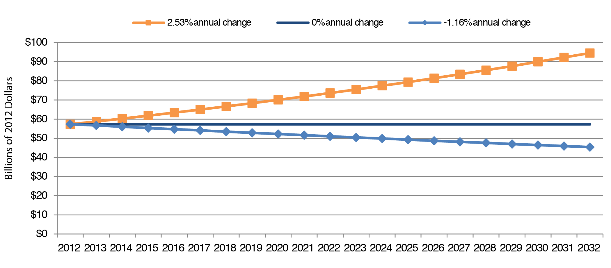
The highest level of spending shown in Exhibit 7-2 corresponds to the annual growth rate in real spending (2.53 percent ) associated with attaining a minimum benefit-cost ratio (BCR) of 1.0 over the 20-year analysis period. As explained in the introduction to Part II of this report, HERS ranks potential projects in order of BCR and implements them until the funding constraint is reached. The lowest BCR among the projects selected, the "marginal BCR," varies across the four funding periods, and HERS refers to the lowest of these values across the funding periods as the "minimum BCR." The attainment of a minimum BCR of 1.0 can be interpreted as having gradually implemented all potentially cost-beneficial projects (BCR ≥ 1.0) over 20 years. The "Improve C&P" reference in Exhibit 7-2 signifies that this level of investment feeds into the Improve Conditions and Performance scenario presented in Chapter 8.

Another funding level shown in Exhibit 7-2 represents the annual growth rate in real spending geared toward matching a specific level of performance in 2032; an average annual growth rate of -1.16 percent is projected to be adequate to allow average pavement roughness as measured by the International Roughness Index (IRI) in 2032 to match the level in 2012 (see discussion of IRI in Chapter 3) and for average delay to be at least as low in 2032 as it was in 2012. This "Maintain C&P" reference in Exhibit 7-2 signifies that this level of investment feeds into the Maintain Conditions and Performance scenario, also presented in Chapter 8.

The remaining four of the six funding levels shown in Exhibit 7-2 represent a range of annual growth rates in real highway spending above, at, and below 2012 funding (2, 1, 0, and -1 percent ). The "2012 Spending" reference in Exhibit 7-2 for the 0.00-percent growth rate row signifies that this level of spending feeds into the Sustain 2012 Spending scenario presented in Chapter 8.

Exhibit 7-2 HERS Annual Investment Levels Analyzed for Federal-Aid Highways

A line graph plots HERS annual investment levels in billions of 2012 dollars at 0%, 2.53%, and -1.16% annual percent changes in HERS capital spending. The HERS level is at $57.4 billion in 2012 and this value is constant at 0% annual change through 2032. For the 2.53% annual percent change, investment levels increase gradually to $65.0 billion at the end of the first funding period (2017). During the second funding period, investment levels increase gradually from $66.6 billion in 2018 to $73.7 billion in 2022. During the third funding period, investment levels increase gradually from $75.5 billion in 2023 to $83.5 billion in 2027. During the fourth funding period, investment levels increase gradually from $85.6 billion in 2028 to $94.6 billion in 2032. For the -1.16% annual percent change, investment levels decrease gradually to $54.1 billion at the end of the first funding period (2017). During the second funding period, investment levels decrease gradually from $53.5 billion in 2018 to $51.1 billion in 2022. During the third funding period, investment levels decrease gradually from $50.5 billion in 2023 to $48.2 billion in 2027. During the fourth funding period, investment levels decrease gradually from $47.6 billion in 2028 to $45.4 billion in 2032. Source: Highway Economic Requirements System.

Annual percent Change in HERS Capital Spending	Spending Modeled in HERS (Billions of 2012 Dollars)								Link to Chapter 8 Scenario
	Cumulative					Average Annual Over 20 Years
	5-Year 2013 Through 2017	5-Year 2018 Through 2022	5-Year 2023 Through 2027	5-Year 2028 Through 2032	20-Year 2013 Through 2032	Total HERS Spending¹	System Rehabilitation Spending²	System Expansion Spending²
2.53%	$309	$351	$397	$450	$1,507	$75.4	$45.4	$30.0	Improve C&P
2.00%	$305	$336	$371	$410	$1,422	$71.1	$43.1	$28.0
1.00%	$296	$311	$326	$343	$1,276	$63.8	$38.7	$25.1
0.00%	$287	$287	$287	$287	$1,147	$57.4	$35.0	$22.4	2012 Spending
-1.00%	$278	$265	$252	$239	$1,034	$51.7	$31.5	$20.2
-1.16%	$277	$261	$247	$233	$1,017	$50.9	$30.9	$19.9	Maintain C&P
¹ The amounts shown represent the average annual investment over 20 years that would occur if annual investment grows in constant dollar terms by the percentage shown in each row of the first column. ² HERS splits its available budget between system rehabilitation and system expansion based on the mix of spending it finds to be most cost-beneficial, which varies by funding level. Source: Highway Economic Requirements System.

The portion of each investment level that HERS directs to system rehabilitation versus system expansion is significant, as these types of investments have varying degrees of influence on different performance measures. Investment in system rehabilitation (ranging from $30.9 billion to $45.4 billion across reported investment levels) tends to have a stronger influence on physical condition measures such as pavement ride quality. Investment in system expansion (ranging from $19.9 billion to $30.0 billion across reported investment levels) has a more pronounced impact on operational performance measures such as delay.

How large is the investment backlog estimated by HERS?

The investment backlog represents all improvements that could be economically justified for immediate implementation, based solely on the current conditions and operational performance of the highway system (without regard to potential future increases in vehicle miles traveled or potential future physical deterioration of pavements).

HERS does not routinely produce rolling backlog figures over time as an output, but is equipped to do special analyses to identify the base-year backlog. To determine which action items to include in the backlog, HERS evaluates the current state of each highway section before projecting the effects of future travel growth on congestion and pavement deterioration. Any potential improvement that would correct an existing pavement or capacity deficiency and that has a benefit-cost ratio greater than or equal to 1.0 is considered part of the current highway investment backlog.

HERS estimates the size of the backlog as $463.1 billion for Federal-aid highways, stated in constant 2012 dollars. The estimated backlog for the Interstate System is $105.1 billion; adding other principal arterials produces an estimated backlog of $281.2 billion for the expanded NHS. The investment levels associated with a minimum benefit-cost ratio of 1.0 presented in this chapter would fully eliminate this backlog and address other deficiencies that arise over the next 20 years, when doing so might be cost-beneficial.

Of note is that these figures reflect only a subset of the total highway investment backlog; they do not include the types of capital improvements modeled in NBIAS (presented later in this chapter) or the types of capital improvements not currently modeled in HERS or NBIAS. Chapter 8 presents an estimate of the combined backlog for all types of improvements (see Exhibit 8-4)

Investment Levels and BCRs by Funding Period

Exhibit 7-2 illustrates how the six alternative funding growth rates for Federal-aid highways that were selected for further analysis in this chapter would translate into cumulative spending in 5year intervals (corresponding to 5-year analysis periods used in HERS). The portions of these investment levels relating to system rehabilitation and system expansion are also identified, as the former would be expected to have a greater impact on measures of physical conditions such as IRI, while the latter would be expected to have a greater impact on measures of operational performance, such as user delay.

As shown in Exhibit 7-2, achieving a minimum BCR of 1.0 is estimated to require $1.507 trillion over the analysis period. Achieving a minimum BCR of 1.0 would necessitate an increase in spending of $360 billion over the analysis period relative to a scenario in which 2012 spending levels were maintained from 2012 through 2032.

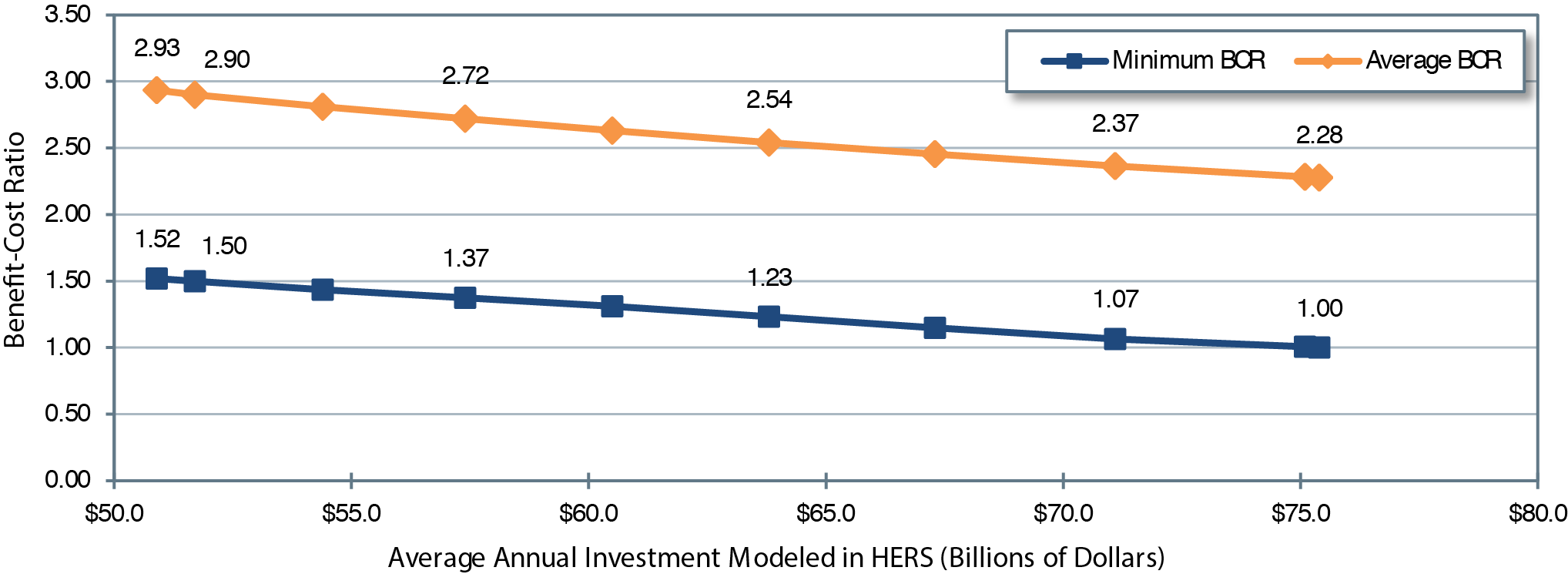
Exhibit 7-3 illustrates the marginal benefit-cost ratios (i.e., the lowest benefit-cost ratio among the improvements selected within a funding period) associated with the six alternative funding levels. Exhibit 7-3 also provides the minimum benefit-cost ratios across all funding periods (which is identical to the lowest marginal benefit-cost ratio) and the average benefit-cost ratios across all funding periods (i.e., the total level of benefits of all improvements divided by the total cost of all improvements). For positive growth rates in spending levels, the marginal BCR declines over time, reflecting the tendency in HERS to implement the most worthwhile improvements first; the minimum BCR over the entire 20-year analysis period, shown in the last column, equals the marginal BCR in the last 5-year period. Conversely, for negative (and zero) growth rates in spending levels, the minimum BCR equals the marginal BCR in the third 5-year period. This pattern reflects the impacts of funding constraints; the relative scarcity of funding toward the end of the analysis period is inadequate to keep pace with newly emerging needs, limiting the range of needs that can be addressed.

Exhibit 7-3 Minimum and Average Benefit-Cost Ratios (BCRs) for Different Possible Funding Levels on Federal-Aid Highways

A line graph plots values for minimum and average benefit-cost ratios over annual investment in billions of dollars modeled in HERS. The plot for minimum BCR has a value of 1.52 at an average annual investment of $50.9 billion, dropping to a value of 1.37 at an investment of $57.4 billion, to a value of 1.23 at an investment of $63.8 billion, to a value of 1.07 at an investment of $71.1 billion, ending at a value of 1.00 at an investment of $75.4 billion. The plot for average BCR has a value of 2.93 at an average annual investment of $50.9 billion, with the trend swinging steadily lower to a value of 2.72 at an investment of $57.4 billion, to a value of 2.54 at an investment of $63.8 billion, to a value of 2.37 at an investment of $71.1 billion, ending at a value of 2.28 at an investment of $75.4 billion. Source: Highway Economic Requirements System.

Average Annual Investment² (Billions of 2012 Dollars)	Average Annual percent Change vs. 2012	Average BCR 20-Year 2013 Through 2032	5-Year 2013 Through 2017	5-Year 2018 Through 2022	5-Year 2023 Through 2027	5-Year 2028 Through 2032	Minimum BCR 20-Year 2013 Through 2032
HERS-Modeled Investment on Federal-Aid Highways		Benefit-Cost Ratios¹						Link to Chapter 8 Scenario
Average Annual Investment² (Billions of 2012 Dollars)	Average Annual percent Change vs. 2012	Average BCR 20-Year 2013 Through 2032	Marginal BCR³				Minimum BCR 20-Year 2013 Through 2032
$75.4	2.53%	2.28	1.80	1.24	1.08	1.00	1.00	Improve C&P
$71.1	2.00%	2.37	1.82	1.27	1.14	1.07	1.07
$63.8	1.00%	2.54	1.86	1.35	1.25	1.23	1.23
$57.4	0.00%	2.72	1.90	1.43	1.37	1.40	1.37	2012 Spending
$51.7	-1.00%	2.90	1.94	1.52	1.50	1.59	1.50
$50.9	-1.16%	2.93	1.95	1.53	1.52	1.62	1.52	Maintain C&P
¹ As HERS ranks potential improvements by their estimated BCRs and assumes that the improvements with the highest BCRs will be implemented first (up until the point where the available budget specified is exhausted), the minimum and average BCRs will naturally tend to decline as the level of investment analyzed rises. ² The amounts shown represent the average annual investment over 20 years that would occur if annual investment grows in constant dollar terms by the percentage shown in each row of the first column. ³ The marginal BCR represents the lowest benefit-cost ratio for any project implemented during the period identified at the level of funding shown. The minimum BCRs, indicated by bold font, are the smallest of the marginal BCRs across the funding periods. Source: Highway Economic Requirements System.

Further evident in Exhibit 7-3 is the inverse relationship between the minimum BCR and the level of investment. At any given level of average annual investment, the average BCR always exceeds the marginal BCR. For example, at the highest level of investment considered, an average annual investment level of $75.4 billion, the average BCR of 2.28 exceeds the minimum BCR of 1.00.

Impact of Future Investment on Highway Pavement Ride Quality

The primary measure of highway physical condition in HPMS is pavement ride quality as measured by IRI (defined in Chapter 3). The HERS analysis presented in this report focuses on VMT-weighted IRI values; the average IRI values shown thus reflect the pavement ride quality experienced on a typical mile traveled. Exhibit 7-4 shows how the projection for the average IRI on Federal-aid highways in 2032 varies with the portion of investment that HERS allocates to system rehabilitation, as identified in Exhibit 7-2; system rehabilitation is more significant than investment in system expansion in influencing average pavement ride quality. The levels of system rehabilitation analyzed range from an average annual investment level of $30.9 billion (which feeds the Maintain Conditions and Performance scenario in Chapter 8) to an average annual investment level of $45.4 billion (which feeds the Improve Conditions and Performance scenario in Chapter 8).

Exhibit 7-4 Projected 2032 Pavement Ride Quality Indicators on Federal-Aid Highways Compared with 2012 for Different Possible Funding Levels

A line graph plots values for VMT on roads with good ride quality and acceptable ride quality in percent for average annual investment in billions of dollars. For roads with good ride quality, the plot has an initial value of 46.0 percent at an annual investment of $30.9 billion, with the trend increasing upward to a value of 46.7 percent at an annual investment of $31.5 billion, 50.8 percent at an annual investment of $35.0 billion, 54.7 percent at an annual investment of $38.7 billion, 58.8 percent at an annual investment of $43.1 billion, ending at value of 60.9 percent at an annual investment of $45.4 billion. For roads with acceptable ride quality, the plot has an initial value of 85.9 percent at an annual investment of $30.9 billion, with the trend increasing upward to a value of 86.2 percent at an annual investment of $31.5 billion, 87.7 percent at an annual investment of $35.0 billion, 89.3 percent at an annual investment of $38.7 billion, 90.8 percent at an annual investment of $43.1 billion, ending at value of 91.5 percent at an annual investment of $45.4 billion. Source: Highway Economic Requirements System.

HERS-Modeled Capital Investment	Projected 2032 Condition Measures on Federal-Aid Highways^1,2				Link to Chapter 8 Scenario
HERS-Modeled Capital Investment	percent of VMT on Roads With Ride Quality of:		Average IRI (VMT-Weighted)
Average Annual for System Rehabilitation (Billions of 2012 Dollars)²	Good (IRI<95)³	Acceptable (IRI<=170)³	Inches Per Mile	Change Relative to Base Year
$45.4	60.9%	91.5%	100.7	-14.0%	Improve C&P
$43.1	58.8%	90.8%	102.9	-12.1%
$38.7	54.7%	89.3%	107.4	-8.3%
$35.0	50.8%	87.7%	111.8	-4.5%	2012 Spending
$31.5	46.7%	86.2%	116.3	-0.7%
$30.9	46.0%	85.9%	117.1	0.0%	Maintain C&P
Base Year Values:	44.9%	83.3%	117.1
¹ The HERS model relies on information from the HPMS sample section database, which is limited to those portions of the road network that are generally eligible for Federal funding (i.e., "Federal-aid highways") and excludes roads classified as rural minor collectors, rural local, and urban local. ² The amounts shown represent only the portion of HERS-modeled spending directed toward system rehabilitation, rather than system expansion. Other types of spending can affect these indicators as well. ³ As discussed in Chapter 3, IRI values of 95 and 170 inches per mile, respectively, are the thresholds associated with "good" and "acceptable" ride quality. Source: Highway Economic Requirements System.

For all investment levels presented in Exhibit 7-4, pavements on Federal-aid highways are projected to be smoother on average in 2032 than in 2012, with the exception of the lowest investment level, which matches the average base-year pavement condition exactly. VMT-weighted average IRI decreases by up to 14 percent across alternatives (from 117.1 to 100.7).

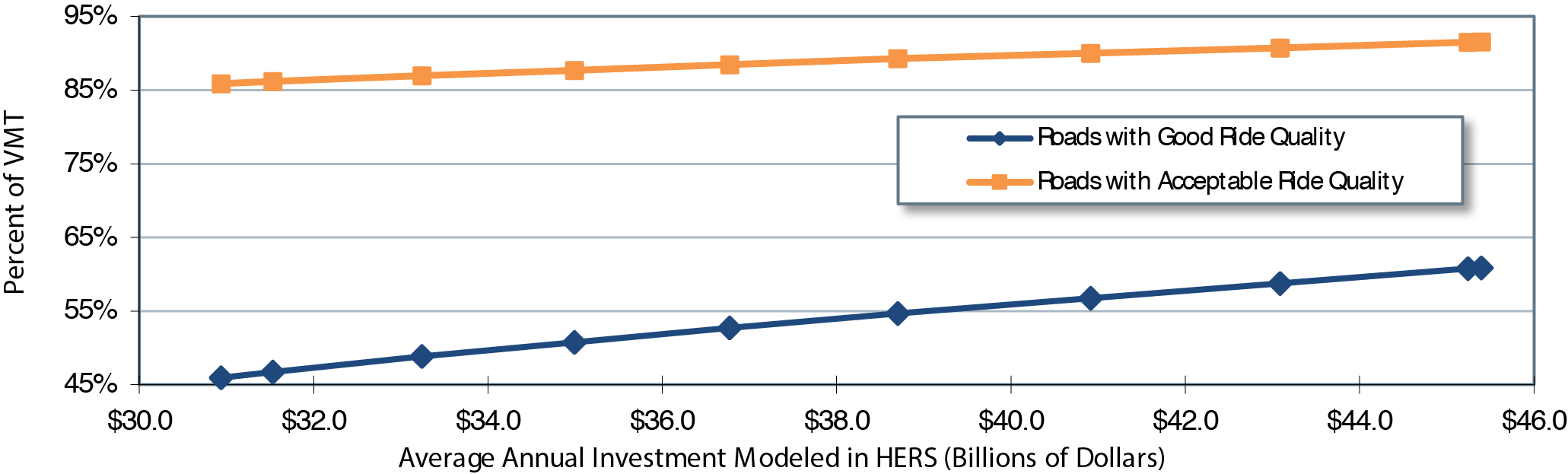
Exhibit 7-4 also shows the HERS projections for the percentage of travel occurring on pavements with ride quality that would be rated good or acceptable based on the IRI thresholds set in Chapter 3. Under all circumstances represented in the exhibit, the 2032 projection for the percentage of travel occurring on pavements with good ride quality exceeds the 44.9 percent that occurred in 2012; the improvement in the share of pavements with good ride quality increases roughly linearly with spending. The projections for 2032 range from 60.9 percent at the highest level of investment modeled (an average annual investment level for system rehabilitation of $45.4 billion) to 46.0 percent at the lowest level of investment (an average annual investment level for system rehabilitation of $30.9 billion).

In all the circumstances considered, Exhibit 7-4 reveals increases relative to the base-year level of 83.3 percent in the proportion of travel occurring on pavements with ride quality rated as acceptable. The projection for 2032 ranges from 91.5 percent at the highest level of investment modeled to 85.9 percent at the lowest. When no change from the 2012 level of investment is modeled, 87.7 percent of travel in 2032 in the forecast traffic growth case is projected to occur on pavements with acceptable ride quality. As noted in Chapter 3, the IRI threshold of 170 used to identify acceptable ride quality was originally set to measure performance on the NHS and might not be fully applicable to non-NHS routes, which tend to have lower travel volumes and speeds.

Why does HERS predict smaller improvements to pavement quality in this report compared to previous analyses?

Two primary factors limit the extent to which future highway investment results in improvements in projected future pavement quality in this report relative to previous analyses. First, the rate of forecast growth in vehicle miles traveled is lower in this analysis than in previous analyses, resulting in the selection of fewer projects that generate improved pavement quality through surface widening. That is, the estimated benefits of widening lanes (with concurrent increases in pavement quality) are reduced relative to the past, because there are fewer projected users to whom benefits would accrue. Second, changes to the pavement model in HERS better reflect the effects of aging road infrastructure and the challenges associated with maintaining pavement quality over time. In particular, revisions to HERS have decreased the rate at which pavement quality is assumed to decline, dampening the estimated benefits of surface rehabilitation projects.

Impact of Future Investment on Highway Operational Performance

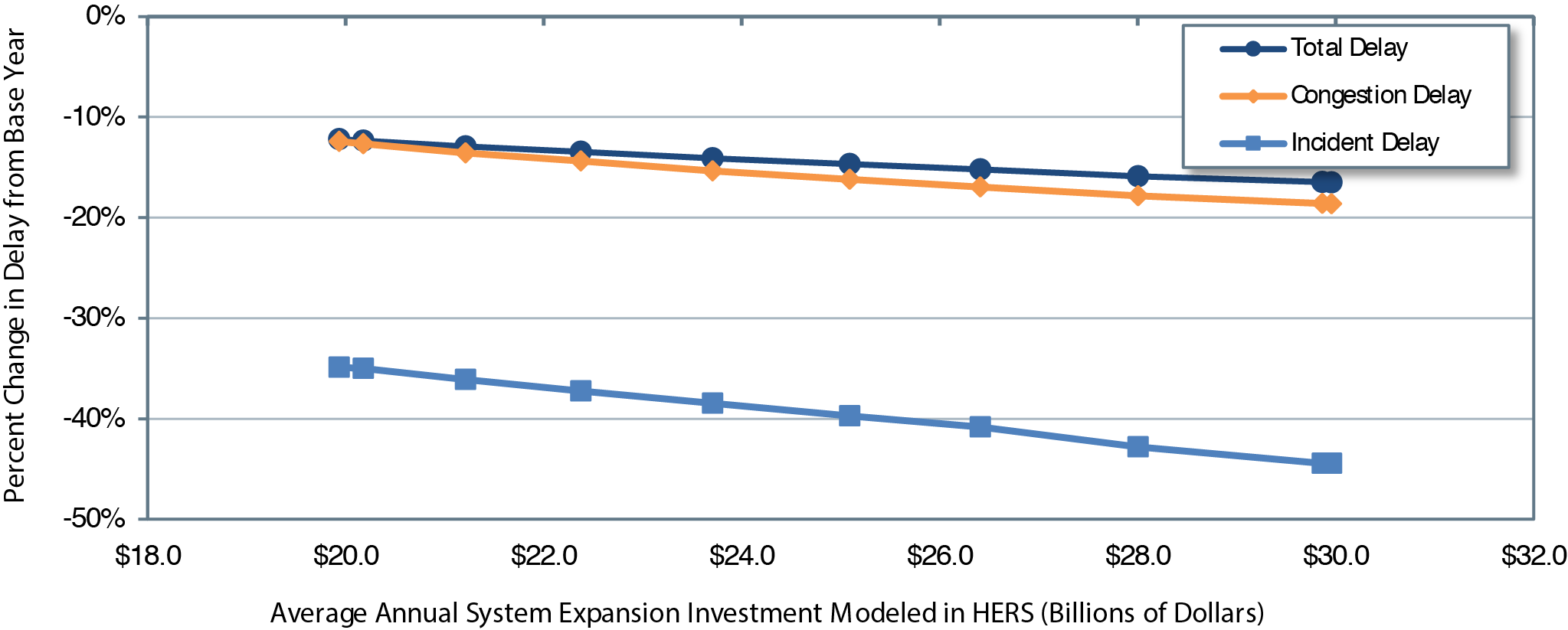
Exhibit 7-5 shows the HERS projections for the impact of investment levels on average speed and traveler delay. Exhibit 7-5 splits out the portion of that investment that HERS programs for system expansion (such as widening existing highways or building new routes in existing corridors), which tend to reduce congestion delay more than spending on system rehabilitation. The levels of system expansion analyzed range from an average annual investment level of $19.9 billion (which feeds the Maintain Conditions and Performance scenario in Chapter 8) to an average annual investment level of $30.0 billion (which feeds the Improve Conditions and Performance scenario in Chapter 8).

Exhibit 7-5 Projected Changes in 2032 Highway Travel Delay and Speed on Federal-Aid Highways Compared with Base Year for Different Possible Funding Levels

A line graph plots values for percent change in delay from the base year in three categories over average annual investment in billions of dollars modeled in HERS. For incident delay, the plot has an initial value of -34.9 percent change at an annual investment of $19.9 billion, trends downward to a value of -37.2 percent change at an annual investment of $22.4 billion, and ends at a value of -44.4 percent change at an annual investment of $30.0 billion. For congestion delay, the plot has an initial value of -12.4 percent change at an annual investment of $19.9 billion, trends downward to a value of -14.4 percent change at an annual investment of $22.4 billion, and ends at a value of -18.6 percent change at an annual investment of $30.0 billion. For total delay, the plot has an initial value of -12.2 percent change at an annual investment of $19.9 billion, trends slowly downward to a value of -13.4 percent change at an annual investment of $22.4 billion, and ends at a value of -16.5 percent change at an annual investment of $30.0 billion. Source: Highway Economic Requirements System; Highway Statistics 2013, Table VM-1.

HERS-Modeled Capital Investment	Projected 2032 Performance Measures on Federal-Aid Highways					Link to Chapter 8 Scenario
HERS-Modeled Capital Investment	Average Speed in 2030 (mph)	Annual Hours of Delay per Vehicle²	percent Change Relative to Baseline
Average Annual System Expansion (Billions of 2012 Dollars)¹	Average Speed in 2030 (mph)	Annual Hours of Delay per Vehicle²	Total Delay per VMT	Congestion Delay per VMT	Incident Delay per VMT
$30.0	44.3	46.0	-16.5%	-18.6%	-44.4%	Improve C&P
$28.0	44.3	46.3	-15.9%	-17.8%	-42.8%
$25.1	44.2	47.0	-14.7%	-16.2%	-39.7%
$22.4	44.0	47.6	-13.4%	-14.4%	-37.2%	2012 Spending
$20.2	43.9	48.2	-12.4%	-12.7%	-35.0%
$19.9	43.9	48.3	-12.2%	-12.4%	-34.9%	Maintain C&P
Base Year Values:	42.3	55.0
¹ The amounts shown represent only the portion of HERS-modeled spending directed toward system expansion rather than system rehabilitation. Other types of spending can affect these indicators as well. ² The values shown were computed by multiplying HERS estimates of average delay per VMT by 11,707, the average VMT per registered vehicle in 2012. HERS does not forecast changes in VMT per vehicle over time. The HERS delay figures include delay attributable to stop signs and signals as well as delay resulting from congestion and incidents. Source: Highway Economic Requirements System; Highway Statistics 2013, Table VM-1.

As noted above, HERS assumes the continuation of existing trends in the deployment of certain system management and operations strategies. Among these strategies are several that can be expected to mitigate delay associated with isolated incidents more than the delay associated with recurring congestion ("congestion delay"), such as freeway incident management programs. In line with this, Exhibit 7-5 shows the amount of incident delay decreasing strongly relative to congestion delay over the period 2012—2032. HERS projects incident delay per VMT on Federal-aid highways to decrease by between 34.9 percent (in the Maintain Conditions and Performance alternative) and 44.4 percent (in the Improve Conditions and Performance alternative) between 2012 and 2032. The results in Exhibit 7-5 also reveal investment within the scope of HERS to be a potent instrument for reducing congestion delay. HERS projects congestion delay to decrease by between 12.4 percent and 16.5 percent .

Why does HERS predict larger reductions in delay in this report compared to previous analyses?

The strong tendency for delay costs to fall is driven by multiple factors. The relatively low forecast growth rate in vehicle miles traveled (VMT) reduces upward pressure on delay compared to previous analyses. Likewise, lower forecast VMT growth enables developments in intelligent transportation systems to mitigate delay more effectively as VMT increases. Improvements in data quality related to obstacles to implementing widening projects improve the ability of HERS to identify economically beneficial projects that add capacity.

Notably, changes to the pavement model have tended to reduce the estimated benefits of pavement improvements, leading to an increased selection rate for projects that add capacity at lower investment levels.

Across all scenarios presented in Exhibit 7-5, annual delay per vehicle in 2032 is lower than the 2012 level (55 hours), with reductions in delay ranging from 6.7 hours in the lowest level of investment analyzed to 9.0 hours in the highest. The projected reductions in delay are associated with relatively small variations in average vehicle speed, ranging from 43.9 miles per hour to 44.3 miles per hour, compared to the 2012 level of 42.3 miles per hour.

Some traffic basics are important to keep in mind when interpreting these results. In addition to congestion and incident delay, some delay inevitably results from traffic control devices. For this reason, and because traffic congestion occurs only at certain places and times, Exhibit 7-5 shows the variation in investment level as having less impact on projections for total delay and average speed than on the projections for congestion and incident delay. In addition, although the impacts of additional investment on average speed are proportionally small, these impacts apply to a vast amount of travel; hence, the associated savings in user cost are not necessarily small relative to the cost of the investment.

Impact of Future Investment on Highway User Costs

In HERS, the benefits from highway improvements are the reductions in highway user costs, agency costs, and societal costs of vehicle emissions. In measuring the highway user costs, the model includes the costs of travel time, vehicle operation, and crashes.

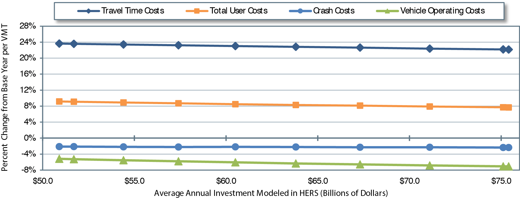
Exhibit 7-6 shows the projected changes from 2012 to 2032 in average user cost of travel on Federal-aid highways by cost component. For Federal-aid highways, HERS estimates that user costs-the costs of travel time, vehicle operation, and crashes-averaged $1.283 per mile traveled in 2012.

Average user cost per VMT is projected to increase at a lower rate at the spending level HERS indicates would be needed to fund all cost-beneficial projects (averaging $75.4 billion annually); under this spending level, average user cost per mile of VMT in 2032 is projected to be $1.382, or 7.7 percent higher than in 2012. Average user cost per VMT is projected to increase between 2012 and 2032 by 8.7 percent and 9.2 percent under the assumptions that real annual spending remains at the base-year level (average annual growth rate of 0.0 percent ) or, alternatively, decreases annually at the rate geared toward maintaining average pavement roughness (1.16 percent ).

Exhibit 7-6 Projected 2032 Average Total User Costs on Federal-Aid Highways Compared with Base Year for Different Possible Funding Levels

A line graph plots values for percent change in average total user costs per VMT on Federal-aid highways from the base year over average annual investment in billions of dollars modeled in HERS. For travel time costs, the plot has an initial value of 23.6 percent change at an annual investment of $50.9 billion and trends slightly downward to end at a value of 22.1 percent change at an annual investment of $75.4 billion. For total user costs, the plot has an initial value of 9.2 percent change at an annual investment of $50.9 billion and travels gradually downward to end at a value of 7.7 percent change at an annual investment of $75.4 billion. For crash costs, the plot has an initial value of -2.1 percent change at an annual investment of $50.9 billion and stays relatively flat to end at a value of -2.3 percent change at an annual investment of $75.4 billion. For vehicle operating costs, the plot has an initial value of -5.2 percent change at an annual investment of $50.9 billion and trends slightly downward to end at a value of -7.1 percent change at an annual investment of $75.4 billion. Source: Highway Economic Requirements System.

HERS-Modeled Investment On Federal-Aid Highways		Projected 2032 Performance Measures on Federal-Aid Highways					Link to Chapter 8 Scenario
Average Annual (Billions of 2012 Dollars)	Average Annual Change vs. 2012	Average Total User Costs ($/VMT)	percent Change Relative to Baseline Average per VMT
Average Annual (Billions of 2012 Dollars)	Average Annual Change vs. 2012	Average Total User Costs ($/VMT)	Total User Costs	Travel Time Costs	Vehicle Operating Costs	Crash Costs
$75.4	2.53%	$1.381	7.7%	22.1%	-7.1%	-2.3%	Improve C&P
$71.1	2.00%	$1.384	7.9%	22.4%	-6.8%	-2.3%
$63.8	1.00%	$1.389	8.3%	22.8%	-6.3%	-2.2%
$57.4	0.00%	$1.394	8.7%	23.2%	-5.8%	-2.2%	2012 Spending
$51.7	-1.00%	$1.399	9.1%	23.6%	-5.3%	-2.1%
$50.9	-1.16%	$1.400	9.2%	23.6%	-5.2%	-2.1%	Maintain C&P
Base Year Values:		$1.283
Source: Highway Economic Requirements System.

The cost of crashes is the user cost component with the lowest absolute sensitivity to the assumed level of highway investment, which as an annual average varies between $50.9 billion (which feeds the Maintain Conditions and Performance scenario in Chapter 8) and $75.4 billion (which feeds the Improve Conditions and Performance scenario in Chapter 8). Crash costs in 2032 are projected to be between 2.1 percent and 2.3 percent lower than in 2012.

The levels of spending in each scenario are limited to the types of improvements that HERS evaluates, which are basically system rehabilitation and expansion. Because HPMS lacks detailed information on the current location and characteristics of safety-related features (e.g., guardrail, rumble strips, roundabouts, yellow change intervals at signals), safety-focused investments are not evaluated. Thus, the findings presented in Exhibit 7-6 establish nothing about how such investments affect highway safety.

Crash costs also form the smallest of the three components of highway user costs. For 2012 travel on Federal-aid highways, HERS estimates the breakdown by cost component to be crash cost, 14.0 percent ; travel time cost, 48.3 percent , and vehicle operating cost, 37.8 percent . Research under way to update the vehicle operating cost equations in HERS (see Appendix A) might alter the split among these costs somewhat, but crash costs will remain a small component. Although highway trips always consume traveler time and resources for vehicle operation, only a small fraction involves crashes. In addition, most crashes are non-catastrophic: Particularly on urban highways, many crashes involve only damage to property with no injuries.

The projections for travel time costs are less sensitive to the assumed level of investment than are the projections for vehicle operating costs. The projected 2012—2032 change in travel time cost per VMT ranges from an increase of 22.1 percent at the highest level of assumed investment to an increase of 23.6 percent at the lowest. These projections indicate that investing at the highest level rather than the lowest level would reduce the time cost of travel per VMT in 2032 by 1.2 percent , saving travelers hundreds of millions of hours per year in aggregate. The projected impacts on travel time costs in this report differ from the corresponding projected impacts in the 2013 C&P Report, which projected a small decrease in travel time cost under high levels of investment. This distinction was driven by assumptions about increasing real travel time costs in future years, as noted previously; the revisions incorporate projected increases in real income, which is a central input to estimated values of travel time savings.

What are the monetized national-level impacts implied by the changes in average user costs projected by HERS?

Exhibit 7-6presents measures of average user costs per vehicle mile traveled (VMT), rather than projections of aggregate, national-level user costs. To identify monetized impacts of changes in investment levels on national-level user costs, national VMT in 2032 can be multiplied by differences in average user costs across investment levels. At the highest level of investment (an annual average of $75.4 billion), average total user costs are projected to be $1.381 per VMT. Average total user costs at the highest level of investment represent decreases in average total user costs of $0.013 per VMT when spending is held at the base-year level ($57.4 billion per year) and $0.019 per VMT at the lowest level of investment (an annual average of $50.9 billion).

Investing at the highest level is projected to result in a decrease in total user costs in 2032 of between $59.6 billion and $60.0 billion relative to the lowest level of investment, depending on the measure of projected VMT specified in the calculation (i.e., the choice of projected VMT among investment levels). Investing at the highest level is projected to result in a decrease in total user costs in 2032 of $40.9 billion relative to investing at the base-year level, for the projected VMT when investing at the lowest level.

Approximately half the projected national-level impacts on average user costs can be attributed to impacts on vehicle operating costs. At the highest investment level, average vehicle operating costs per VMT in 2032 are projected to be $0.009 lower than under the lowest investment level and $0.006 lower than when spending is held at the base-year level. Investing at the highest level is projected to result in a decrease in total vehicle operating costs in 2032 of $28.3 relative to the lowest level of investment, based on projected VMT for the lowest investment level in 2032. Investing at the highest level is projected to result in a decrease in total vehicle operating costs in 2032 of $18.9 billion relative to investing at the base-year level, based on projected VMT for the lowest investment level in 2032.

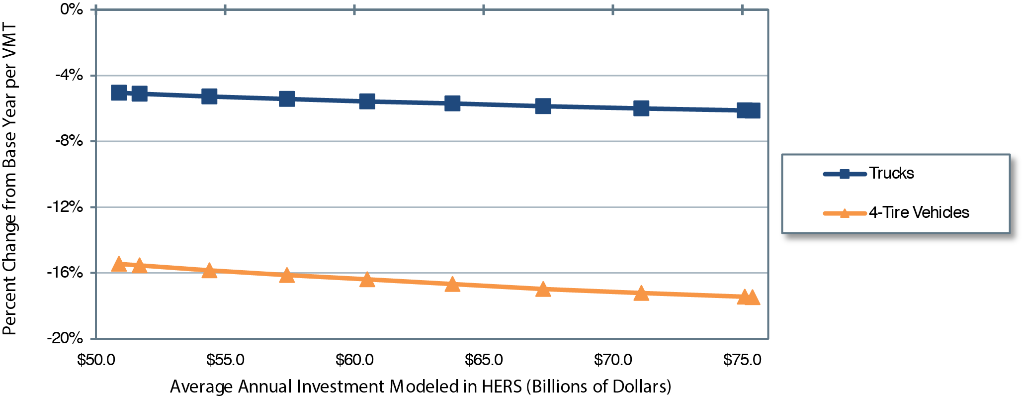
Impact on Vehicle Operating Costs

Exhibit 7-7 presents projections for vehicle operating costs per VMT, including separate values for four-tire vehicles (light-duty vehicles) and trucks (heavy-duty vehicles). The projected 2012—2032 change in vehicle operating costs per VMT ranges from a decrease of 5.2 percent at the lowest level of assumed investment (from $0.485 to $0.460 per VMT) to a decrease of 7.0 percent at the highest (from $0.485 to $0.451 per VMT). These projections indicate that investing at the highest level rather than at the lowest level would reduce the operating cost of travel per VMT in 2032 by 2.0 percent (from $0.460 to $0.451 per VMT).

Exhibit 7-7 Projected 2032 Vehicle Operating Costs on Federal-Aid Highways Compared with Base Year for Different Possible Funding Levels

A line graph plots values for percent change in average vehicle operating costs per VMT from the base year over average annual investment in billions of dollars modeled in HERS for trucks and 4-tire vehicles. For trucks, the plot has an initial value of -5.1 percent change at an annual investment of $50.9 billion and trends downward gradually to end at a value of -6.1 percent change at an annual investment of $75.4 billion. For 4-tire vehicles, the plot has an initial value of -15.5 percent change at an annual investment of $50.9 billion and trends downward steadily to reach a value of -17.5 percent change at an annual investment of $75.4 billion. Source: Highway Economic Requirements System.

HERS-Modeled Investment on Federal-Aid Highways		Projected 2032 Performance Measures on Federal-Aid Highways					Link to Chapter 8 Scenario
Average Annual Investment (Billions of 2012 Dollars)	Average Annual percent Change vs. 2012	Average Vehicle Operating Costs			percent Change Relative to Baseline
Average Annual Investment (Billions of 2012 Dollars)	Average Annual percent Change vs. 2012	All Vehicles ($/VMT)	4-Tire Vehicles ($/VMT)	Trucks ($/VMT)	4-Tire Vehicles	Trucks
$75.4	2.53%	$0.451	$0.342	$1.087	-17.5%	-6.1%	Improve C&P
$71.1	2.00%	$0.452	$0.343	$1.089	-17.2%	-6.0%
$63.8	1.00%	$0.454	$0.346	$1.092	-16.7%	-5.7%
$57.4	0.00%	$0.457	$0.348	$1.096	-16.1%	-5.4%	2012 Spending
$51.7	-1.00%	$0.459	$0.350	$1.099	-15.5%	-5.1%
$50.9	-1.16%	$0.460	$0.351	$1.100	-15.5%	-5.1%	Maintain C&P
Base Year Values:		$0.485
Source: Highway Economic Requirements System.

The projected impacts on vehicle operating costs are larger for four-tire vehicles than for trucks when compared to both the 2012 values and the adjusted baseline. When comparing the vehicle operating cost projections to the adjusted baseline, the magnitudes of the impacts are much larger; isolating the effects of future highway investment reveals that vehicle operating costs per mile are projected to decline by between 15.5 percent and 17.5 percent for four-tire vehicles, and by between 5.1 percent and 6.1 percent for trucks from 2012 to 2032.

The projected reductions in vehicle operating costs per VMT are driven by projected increases in fuel efficiency across the analysis horizon. The assumed paths of fuel efficiency are based on projections from the Energy Information Administration's Annual Energy Outlook 2014. The average price of gasoline is assumed to decrease between 2012 and 2032 by 4.7 percent relative to the consumer price index, while the average price of diesel fuel is assumed to increase by 9.2 percent relative to the consumer price index. The projected changes in fuel prices are added to the fuel cost savings that would result from the improvements in vehicle energy efficiency that the Energy Information Administration projects for this same period; these changes are represented in HERS as increases in average miles per gallon (mpg) of 54.6 percent for light-duty vehicles, 53.9 percent for two-axle trucks, and 15.5 percent for trucks with three or more axles. These projections incorporate the effect of increases in Corporate Average Fuel Economy (CAFE) standards and U.S. Environmental Protection Agency (EPA) standards for emissions of greenhouse gases by automobiles and light trucks through model year 2025. The projections also account for new standards for fuel efficiency and greenhouse gas emissions for medium- and heavy-duty trucks through model year 2018 adopted by the U.S. Department of Transportation and EPA.

What changes in CAFE standards have recently been adopted, and what impacts are these changes expected to have?

On May 7, 2010, the National Highway Traffic Safety Administration (NHTSA) and U.S. Environmental Protection Agency (EPA) jointly adopted Corporate Average Fuel Economy (CAFE) and carbon dioxide (CO) emission standards for cars and light trucks produced during model years 2012 through 2016. In combination with NHTSA's previous actions, this rule raised required fleet-average fuel economy levels for cars from 27.5 miles per gallon (mpg) in model year 2010 to 37.8 mpg for model year 2016, and those for light trucks from 23.5 mpg in 2010 to 28.8 mpg for 2016. On August 28, 2012, the two agencies adopted new rules that further increased CAFE standards for model year 2021 to 46.1 to 46.8 mpg for automobiles and to 32.6 to 33.3 mpg for light trucks; this most recent action also established tentative CAFE standards for model year 2025 of 55.3 to 56.2 mpg for cars and 39.3 to 40.3 mpg for light trucks. All of the adopted and tentative CAFE standards apply to the vehicle fleet as a whole, and are minimum standards for the vehicle fleet.

The impacts of these standards on the fuel economy of the overall vehicle fleet will continue to grow for many years beyond 2025, as new vehicles meeting the higher fuel economy requirements gradually replace older, less fuel-efficient vehicles. In announcing the most recent increases in CAFE standards, NHTSA estimated that the cumulative effects of its actions would be to save more than 500 billion gallons of fuel and to reduce COemissions by 6 billion metric tons over the lifetimes of cars and light trucks produced in 2011 through 2025. The agency also estimated that its standards would save the Nation's drivers more than $1.7 trillion in fuel costs over these vehicles' lifetimes.

In 2011, NHTSA and EPA also established new fuel efficiency and COemission standards for medium- and heavy-duty trucks produced from 2014 through 2018. These standards are expected to reduce fuel consumption by an additional 22 billion gallons, while further reducing COemissions by nearly 270 million metric tons.

Impact of Future Investment on Future VMT

As discussed above, the travel demand elasticity features in HERS modify future VMT growth for each HPMS sample section based on changes to highway user costs. In the absence of information to the contrary, previous C&P reports assumed that the HPMS forecasts represented the level of travel that would occur if user costs did not change. Because the baseline VMT forecasts used in this report are tied to a specific VMT forecasting model with known inputs, this assumption was changed. For this report, HERS was programmed to assume that the baseline projections of future VMT already accounted for anticipated independent changes in user cost component values.

In computing the impact of user cost changes on future VMT growth on an HPMS sample section, HERS compares projected highway user costs against assumed user costs that would have occurred had the physical conditions or operating performance on that highway section remained unchanged. This concept is illustrated in Exhibit 7-8. Based on the 2012 values assigned to various user cost components (e.g., value of travel time per hour, fuel prices, fuel efficiency, truck travel as a percentage of total travel), HERS computes baseline 2012 user costs at $1.283 per mile. If the 2032 values assigned to those same user cost components were applied in 2012, however, HERS would compute 2012 user costs to be $1.437 per mile. This "adjusted baseline" is the relevant point of comparison when examining the impact of user cost changes on VMT.

Exhibit 7-8 Projected 2032 User Costs and VMT on Federal-Aid Highways Compared with Base Year for Different Possible Funding Levels
HERS-Modeled Investment on Federal-Aid Highways		Projected 2032 Indicators on Federal-Aid Highways					Link to Chapter 8 Scenario
Average Annual Investment (Billions of 2012 Dollars)	Average Annual percent Change vs. 2012	Average Total User Costs¹			Projected VMT²
		($/VMT)	percent Change		Trillions of VMT	Annual percent Change vs. 2012
		($/VMT)	vs. Actual 2012	vs. Adjusted Baseline	Trillions of VMT	Annual percent Change vs. 2012
$75.4	2.53%	$1.381	7.7%	-3.9%	3.160	1.15%	Improve C&P
$71.1	2.00%	$1.384	7.9%	-3.7%	3.157	1.15%
$63.8	1.00%	$1.389	8.3%	-3.3%	3.151	1.14%
$57.4	0.00%	$1.394	8.7%	-3.0%	3.145	1.13%	2012 Spending
$51.7	-1.00%	$1.399	9.1%	-2.6%	3.140	1.12%
$50.9	-1.16%	$1.400	9.2%	-2.6%	3.139	1.12%	Maintain C&P
Base Year Values:		$1.283			2.513	1.04%
Adjusted Baseline:		$1.437
¹ The computation of user costs includes several components (value of travel time per hour, fuel prices, fuel efficiency, truck travel as a percent of total travel, etc.) that are assumed to change over time independently of future highway investment. The adjusted baseline applies the parameter values for 2032 to the data for 2012 so that changes in user costs attributable to future highway investment can be identified. ² The operation of the travel demand elasticity features in HERS cause future VMT growth to be influenced by future changes in average user costs per VMT. For this report, the model was set to assume that the baseline projections of future VMT already took into account anticipated independent future changes in user cost component values; hence, it is the changes versus the adjusted baseline user costs that are relevant. Since the percentage change in adjusted total user costs declined for each of the investment levels identified, the annual projected VMT growth was higher than the 1.04-percent baseline projection in all cases. Source: Highway Economic Requirements System.

Although user costs are projected to increase in absolute terms from 2012 to 2032, they are projected to decline relative to the adjusted baseline by between 2.6 percent (at the lowest level of investment analyzed) and 3.9 percent (at the highest level of investment analyzed in 2032). Because the percentage change in adjusted total user costs declined for each investment level identified, the effective annual projected VMT growth associated with each investment level was higher than the 1.04 percent baseline projection in all cases, ranging from 1.12 percent to 1.15 percent .

Impacts of NHS Investments Modeled by HERS

As described in Chapter 2, the NHS includes the Interstate System and other routes most critical to national defense, mobility, and commerce. As noted earlier, the NHS analyses presented in this section are based on an estimate of what the NHS will look like after its expansion pursuant to MAP-21, rather than the system as it existed in 2012.

This section examines the impacts that investment on NHS roads could have on future NHS conditions and performance, independently of spending on other Federal-aid highways. The analysis presented in this section centers on HERS runs that used a database consisting only of NHS roads. This process differs from that used in previous reports, in which the levels of future investment in NHS roads were extracted from analyses that compared potential investments across a database of all Federal-aid highways. The estimated annual growth rates of investment levels for the NHS are different from those of Federal-aid highways above, because the trade-offs among costs and corresponding benefits of potential improvements are not identical across the two sets of roadways. The investment levels presented in this section were selected by applying the operational constraints used in the analysis of all Federal-aid roads (e.g., average annual spending growth rates, minimum BCR, maintaining pavement roughness, and average delay at the base-year level) to the NHS-specific database.

Impact of Future Investment on NHS User Costs and VMT

Exhibit 7-9 presents the projected impacts of NHS investment on VMT and total average user costs on NHS roads in 2032. Average user costs are projected to be lower in 2032 than for the adjusted baseline ($1.367 per VMT) for all investment levels presented. When increasing spending gradually over 20 years to implement all cost-beneficial projects (the highest level of investment, an annual average of $53.0 billion), average total user costs are projected to be 5.0 percent lower ($1.299 per VMT) than in 2012. At the lowest level of investment presented (an annual average of $36.5 billion), average total user costs are projected to be 3.4 percent lower ($1.320 per VMT) than in 2012.

Projected VMT growth on NHS roads is relatively insensitive to the range of investment levels presented in Exhibit 7-9. At the highest level of investment presented in Exhibit 7-9 (an annual average of $53.0 billion), VMT is projected to grow at an average annual rate of 1.18 percent from 2012 to 2032 (2.071 trillion VMT in 2032 versus 1.638 trillion VMT in 2012). At the lowest level of investment presented in Exhibit 7-9 (an annual average of $36.5 billion), VMT is projected to grow at an average annual rate of 1.14 percent from 2012 to 2032 (2.056 trillion VMT in 2032 versus 1.638 trillion VMT in 2012).

Exhibit 7-9 HERS Investment Levels Analyzed for the National Highway System and Projected Minimum Benefit-Cost Ratios, User Costs, and Vehicle Miles Traveled
HERS-Modeled Investment On the NHS				Projected NHS Indicators			Link to Chapter 8 Scenario
Average Annual percent Change vs. 2012	Average Annual Over 20 Years			Minimum BCR 20-Year 2013 through 2032³	Average 2032 Total User Costs ($/VMT)⁴	Projected 2032 VMT (Trillions)⁵
Average Annual percent Change vs. 2012	Total HERS Spending¹	System Rehabilitation Spending²	System Expansion Spending²	Minimum BCR 20-Year 2013 through 2032³	Average 2032 Total User Costs ($/VMT)⁴	Projected 2032 VMT (Trillions)⁵
2.52%	$53.0	$29.8	$23.2	1.00	$1.299	2.071	Improve C&P
2.00%	$50.0	$28.4	$21.7	1.06	$1.302	2.068
1.00%	$44.9	$25.4	$19.5	1.20	$1.308	2.064
0.00%	$40.4	$22.8	$17.6	1.29	$1.314	2.060	2012 Spending
-0.38%	$38.9	$21.9	$17.0	1.33	$1.316	2.059	Maintain C&P
-1.00%	$36.5	$20.4	$16.0	1.39	$1.320	2.056
			Base Year Values:		$1.222	1.638
			Adjusted Baseline:		$1.367
¹ The amounts shown represent the average annual investment over 20 years that would occur if annual investment grows in constant dollar terms by the percentage shown in each row of the first column. ² HERS splits its available budget between system rehabilitation and system expansion based on the mix of spending it finds to be most cost-beneficial which varies by funding level. ³ As HERS ranks potential improvements by their estimated BCRs and assumes that the improvements with the highest BCRs will be implemented first (up until the point where the available budget specified is exhausted), the minimum BCR will naturally tend to decline as the level of investment analyzed rises. ⁴ The computation of user costs includes several components (value of travel time per hour, fuel prices, fuel efficiency, truck travel as a percent of total travel, etc.) that are assumed to change over time independently of future highway investment. The adjusted baseline applies the parameter values for 2032 to the data for 2012, so that changes in user costs attributable to future highway investment can be identified. ⁵ The operation of the travel demand elasticity features in HERS cause future VMT growth to be influenced by future changes in average user costs per VMT. For this report, the model was set to assume that the baseline projections of future VMT already took into account anticipated independent future changes in user cost component values; hence, it is the changes versus the adjusted baseline user costs that are relevant. Source: Highway Economic Requirements System.

Across the investment levels presented in Exhibit 7-9, HERS allocates between $20.4 billion and $29.8 billion in average annual spending on NHS roads to system rehabilitation and between $16.0 billion and $23.2 billion in average annual spending on NHS roads to system expansion.

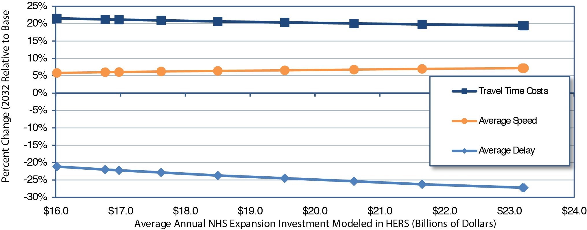
Impact of Future Investment on NHS Travel Times and Travel Time Costs

Exhibit 7-10 presents the projections of NHS averages for time-related indicators of performance, along with the spending amount that HERS programs for NHS expansion projects (which have stronger effects on time-related indicators of performance than preservation projects have). For all investment levels presented in Exhibit 7-10, average travel speed in 2032 exceeds average travel speed in 2012 (48.3 miles per hour). The range of average travel speeds is narrow across the investment levels. At the lowest level of investment in system expansion presented in Exhibit 7-10 (an annual average of $16.0 billion), the average travel speed in 2032 is projected to be 51.1 miles per hour. At the highest level of investment in system expansion presented in Exhibit 7-10 (an annual average of $23.2 billion), the average travel speed in 2032 is projected to be 51.8 miles per hour.

Exhibit 7-10 Projected Changes in 2032 Highway Speed, Travel Delay, and Travel Time Costs on the National Highway System Compared with Base Year for Different Possible Funding Levels

A line graph plots values for percent change in delay from the base year in three categories over average annual investment in billions of year 2012 dollars modeled in HERS. For travel time costs, the plot has an initial value of 21.5 percent change at an annual investment of $16.0 billion, reaches 21.1 percent change at an annual investment of $17.0 billion, continues downward to a value of 20.9 percent change at an annual investment of $17.6 billion, begins to level out at a value of 20.3 percent change at an annual investment of $19.5 billion, continues downward to a value of 19.8 percent change at an annual investment of $21.7 billion, and ends at a value of 19.4 percent change at an annual investment of $23.2 billion. For average speed, the plot has an initial value of 5.8 percent change at an annual investment of $16.0 billion, reaches 6.1 percent change at an annual investment of $17.0 billion, continues upward to a value of 6.2 percent change at an annual investment of $17.6 billion, reaches a value of 6.6 percent change at an annual investment of $19.5 billion, continues upward to a value of 7.0 percent change at an annual investment of $21.7 billion, and ends at a value of 7.2 percent change at an annual investment of $23.2 billion. For average delay, the plot has an initial value of minus 21.2 percent change at an annual investment of $16.0 billion, reaches minus 22.2 percent change at an annual investment of $17.0 billion, continues downward to a value of minus 22.9 percent change at an annual investment of $17.6 billion, trending down to a value of minus 24.5 percent change at an annual investment of $19.5 billion, continuing downward to a value of minus 26.3 percent change at an annual investment of $21.7 billion, and ends at a value of minus 27.2 percent change at an annual investment of $23.2 billion. Source: Highway Economic Requirements System; Highway Statistics 2013, Table VM-1.

HERS-Modeled Investment on the NHS	Projected 2032 Performance Measures on the NHS				Link to Chapter 8 Scenario
Average Annual for System Expansion (Billions of 2012 Dollars)¹	Average Speed (mph)	percent Change Relative to Baseline
	Average Speed (mph)	Average Speed	Average Delay per VMT	Travel Time Costs per VMT²
$23.2	51.8	7.2%	-27.2%	19.4%	Improve C&P
$21.7	51.7	7.0%	-26.3%	19.8%
$19.5	51.5	6.6%	-24.5%	20.3%
$17.6	51.3	6.2%	-22.9%	20.9%	2012 Spending
$17.0	51.2	6.1%	-22.2%	21.1%	Maintain C&P
$16.0	51.1	5.8%	-21.2%	21.5%
Base Year Values:	48.3
¹ The amounts shown represent only the portion of HERS-modeled spending directed toward system expansion, rather than system rehabilitation. Other types of spending can affect these indicators as well. ² Travel time costs are affected by an assumption that the value of time will increase by 1.2 percent in real terms each year. Hence, costs would rise even if travel time remained constant. Source: Highway Economic Requirements System; Highway Statistics 2013, Table VM-1.

The global increase in average travel speed across investment levels corresponds with large decreases in average delay per VMT across investment levels. At the highest level of investment in system expansion presented in Exhibit 7-10, average delay per VMT in 2032 is projected to be 27.2 percent lower than in 2012. At the lowest level of investment in system expansion presented in Exhibit 7-10, average delay per VMT in 2032 is projected to be 21.2 percent lower than in 2012.

Due to increases in the value of time from 2012 to 2032, the projected increases in average travel speed do not correspond to decreases in travel time costs per VMT. Travel time costs per VMT in 2032 are projected to increase across the investment levels presented. Travel time costs per VMT in 2032 are projected to increase by 19.4 percent relative to 2012 at the highest investment level and to increase by 21.5 percent at the lowest level of investment.

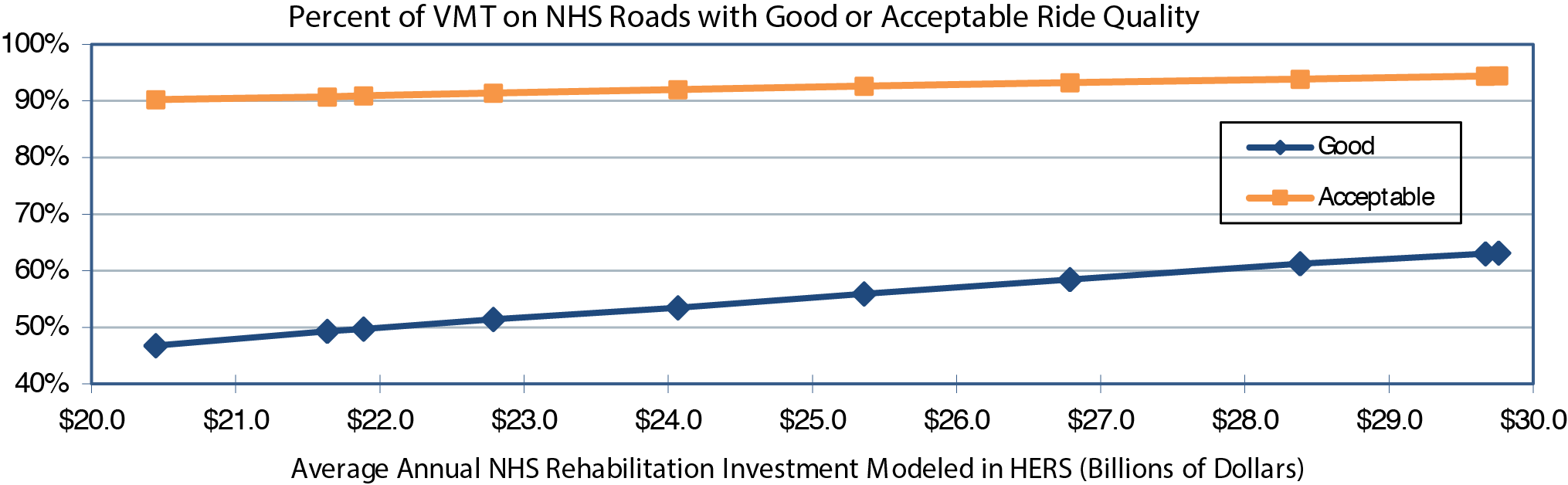
Impact of Future Investment on NHS Pavement Ride Quality

Exhibit 7-11 shows the portion of modeled NHS spending that HERS allocates to rehabilitation projects (which influence average pavement quality more than expansion projects do). The projected average pavement roughness of NHS roads is sensitive to the level of investment on NHS roads. At the highest level of investment presented in Exhibit 7-11 (an annual average of $29.8 billion allocated to system rehabilitation), the model projects average pavement roughness on the NHS to be 12.0 percent lower in 2032 than in 2012. At the lowest level of investment presented in Exhibit 7-11 (an annual average of $20.4 billion allocated to system rehabilitation), the model projects average pavement roughness on the NHS to be 2.5 percent higher in 2032 than in 2012.

Exhibit 7-11 Projected 2032 Pavement Ride Quality Indicators on the National Highway System Compared with 2012 for Different Possible Funding Levels

A line graph plots values for VMT on roads with good or acceptable ride quality in percent over average annual NHS rehabilitation investment in billions of dollars modeled in HERS. For the share of roads with good ride quality, the plot has an initial value of 46.8 percent of VMT at an annual investment of $20.4 billion, with the trend swinging upward to a value of 49.7 percent of VMT at an annual investment of $21.9 billion, continuing upward to 51.4 percent of VMT at an annual investment of $22.8 billion, ending at value of 63.1 percent of VMT at an annual investment of $29.8 billion. For the share of roads with acceptable ride quality, the plot has an initial value of 90.2 percent of VMT at an annual investment of $20.4 billion, with the trend swinging upward to a value of 90.9 percent of VMT at an annual investment of $21.9 billion, continuing upward to 91.4 percent of VMT at an annual investment of $22.8 billion, ending at value of 94.4 percent of VMT at an annual investment of $29.8 billion. Source: Highway Economic Requirements System.

HERS-Modeled Investment on the NHS	Projected 2032 Condition Measures on the NHS¹				Link to Chapter 8 Scenario
Average Annual for System Rehabilitation (Billions of 2012 Dollars)²	percent of VMT on Roads With Ride Quality of:		Average IRI (VMT-Weighted)
	Good (IRI<95)	Acceptable (IRI<=170)	Inches Per Mile	Change Relative to Base Year
$29.8	63.1%	94.4%	94.6	-12.0%	Improve C&P
$28.4	61.2%	93.8%	96.5	-10.2%
$25.4	55.9%	92.6%	101.5	-5.6%
$22.8	51.4%	91.4%	105.8	-1.6%	2012 Spending
$21.9	49.7%	90.9%	107.5	0.0%	Maintain C&P
$20.4	46.8%	90.2%	110.2	2.5%
Base Year Values:	57.1%	89.0%	107.5
¹ As discussed in Chapter 3, IRI values of 95 and 170 inches per mile, respectively, are the thresholds associated with "good" and "acceptable" pavement ride quality on the NHS. ² The amounts shown represent only the portion of HERS-modeled spending directed toward system rehabilitation, rather than system expansion. Other types of spending can affect these indicators as well. Source: Highway Economic Requirements System.

At the highest level of investment presented in Exhibit 7-11, the model projects that pavements with an IRI below 95, which was the criterion in Chapter 3 for rating ride quality as "good," will carry 63.1 percent of the VMT on the NHS, up from the 57.1 percent estimated for 2012. At this investment level, the average IRI of the system would be 94.6, achieving the classification of providing good ride quality at the aggregate level. Furthermore, at the highest level of investment presented in Exhibit 7-11, HERS projects that 94.4 percent of VMT on the NHS would be on roads with an IRI at or below 170, which was the criterion in Chapter 3 for rating ride quality as "acceptable." This projection represents an improvement of 5.4 percentage points in the share of NHS roads with acceptable ride quality relative to the base year (89.0 percent of NHS roads with acceptable ride quality).

At the lowest level of investment presented in Exhibit 7-11, the model projects that pavements with an IRI below 95 will carry 46.8 percent of the VMT on the NHS, down from the 57.1 percent estimated for 2012. At this investment level, the average IRI of the system would increase to 110.2, which fails to achieve the classification of providing good ride quality at the aggregate level. The share of NHS roads with acceptable ride quality is projected to increase slightly by 2032 at the lowest level of investment presented in Exhibit 7-11; HERS projects that 90.2 percent of VMT on the NHS would be on roads with an IRI at or below 170, which is slightly higher than the share of NHS roads with acceptable ride quality in 2012 (89.0 percent of NHS roads with acceptable ride quality).

Based on these modeling results, additional investment to bring the percentage of NHS VMT on roads with "good" or "acceptable" ride quality closer to 100 percent would be economically inefficient, as the costs would exceed the benefits. A key factor leading to this result is that some improvements are not cost-beneficial until IRI rises above the threshold for acceptable ride quality by a sufficient margin. Thus, for some roads with an IRI above 170, improvements would not generate benefits exceeding costs. A further restriction in achieving a state in which all roads have an IRI at or below 170 is that, at any given point, some pavements will be under construction.

Impacts of Interstate System Investments Modeled by HERS

The Interstate System, unlike the broader NHS of which it is a part, has standard design and signage requirements, making it the most recognizable subset of the highway network. This section examines the impacts that investment in the Interstate System could have on future Interstate System conditions and performance, independently of spending on other Federal-aid highways. The analysis presented in this section centers on HERS runs that used a database consisting only of Interstate System roads. This process differs from that used in previous reports, in which the levels of future investment in the Interstate System were extracted from analyses that compared potential investments across a database of all Federal-aid highways.

The Interstate investment levels presented in this section were selected by applying the operational constraints used in the analysis of all Federal-aid roads (e.g., average annual spending growth rates, minimum BCR, maintaining pavement roughness, and average delay at the base-year level) to the Interstate System-specific database.

Impact of Future Investment on Interstate User Costs and VMT

Exhibit 7-12 presents the projected impacts of highway investment on VMT and total average user costs on Interstate roads in 2032, along with the amount that HERS allocates to Interstate projects. Average user costs are projected to be lower in 2032 than the adjusted baseline ($1.267 per VMT) for all investment levels presented. At the highest level of investment presented in Exhibit 7-12 (an annual average of $23.7 billion), average total user costs are projected to be 4.9 percent lower ($1.205 per VMT) than in 2012. At the lowest level of investment presented (an annual average of $13.7 billion), average total user costs are projected to be 2.1 percent lower ($1.241 per VMT) than in 2012.

Exhibit 7-12 HERS Investment Levels Analyzed for the Interstate System and Projected Minimum Benefit-Cost Ratios, User Costs, and Vehicle Miles Traveled
HERS-Modeled Investment On the Interstate System				Projected Interstate Indicators			Link to Chapter 8 Scenario
Average Annual percent Change vs. 2012	Average Annual Over 20 Years			Minimum BCR 20-Year 2013 through 2032³	Average 2032 Total User Costs ($/VMT)⁴	Projected 2032 VMT (Trillions)⁵

	Total HERS Spending¹	System Rehabilitation Spending²	System Expansion Spending²
4.08%	$23.7	$12.7	$11.0	1.00	$1.205	0.926	Improve C&P
4.00%	$23.5	$12.6	$10.9	1.01	$1.205	0.926
3.00%	$21.0	$11.4	$9.6	1.12	$1.212	0.923
2.00%	$18.8	$10.3	$8.5	1.25	$1.219	0.921
1.74%	$18.3	$10.1	$8.2	1.26	$1.222	0.920	Maintain C&P
1.00%	$16.9	$9.3	$7.6	1.37	$1.226	0.919
0.00%	$15.2	$8.3	$6.8	1.54	$1.234	0.917	2012 Spending
-1.00%	$13.7	$7.6	$6.1	1.66	$1.241	0.915
Base Year Values:					$1.129	0.728
Adjusted Baseline:					$1.267
¹ The amounts shown represent the average annual investment over 20 years that would occur if annual investment grows in constant dollar terms by the percentage shown in each row of the first column. ² HERS splits its available budget between system rehabilitation and system expansion based on the mix of spending it finds to be most cost-beneficial which varies by funding level. ³ As HERS ranks potential improvements by their estimated BCRs and assumes that the improvements with the highest BCRs will be implemented first (up until the point where the available budget specified is exhausted), the minimum BCR will naturally tend to decline as the level of investment analyzed rises. ⁴ The computation of user costs includes several components (value of travel time per hour, fuel prices, fuel efficiency, truck travel as a percent of total travel, etc.) that are assumed to change over time independent of future highway investment. The adjusted baseline applies the parameter values for 2032 to the data for 2012 so that changes in user costs attributable to future highway investment can be identified. ⁵ The operation of the travel demand elasticity features in HERS cause future VMT growth to be influenced by future changes in average user costs per VMT. For this report, the model was set to assume that the baseline projections of future VMT already took into account anticipated independent future changes in user cost component values; hence, it is the changes versus the adjusted baseline user costs that are relevant. Source: Highway Economic Requirements System.

Projected VMT growth on Interstate roads is relatively insensitive to the range of investment levels presented in Exhibit 7-12. At the highest level of investment presented in Exhibit 7-12 (an annual average of $23.7 billion), VMT is projected to grow at an average annual rate of 1.21 percent from 2012 to 2032 (926 billion VMT in 2032 versus 728 billion VMT in 2012). At the lowest level of investment presented in Exhibit 7-12 (an annual average of $13.7 billion), VMT is projected to grow at an average annual rate of 1.15 percent from 2012 to 2032 (915 billion VMT in 2032 versus 728 billion VMT in 2012).

Across the investment levels presented in Exhibit 7-12, HERS allocates between $7.6 billion and $12.7 billion in average annual spending on Interstate roads to system rehabilitation, and between $6.1 billion and $11.0 billion in average annual spending on Interstate roads to system expansion.

Impact of Future Investment on Interstate System Travel Times and Travel Costs

Exhibit 7-13 presents the projections of Interstate System averages for time-related indicators of performance, along with the amount that HERS programs for Interstate System expansion projects (which have a relatively large impact on travel time). Across all investment levels presented in Exhibit 7-13, average speed on the Interstate System is projected to be higher than its 2012 level (61.6 miles per hour) in 2032. At the highest level of investment presented in Exhibit 7-13 (average annual investment in system expansion of $11.0 billion), average Interstate highway travel speed is projected to be 8.9 percent higher (67.1 miles per hour) in 2032 than in 2012. At the lowest level of investment presented in Exhibit 7-13 (average annual investment in system expansion of $6.1 billion), average Interstate highway travel speed is projected to be 5.3 percent higher (64.9 miles per hour) in 2032 than in 2012.

The global increase in average travel speed across investment levels corresponds with large decreases in average delay per VMT across investment levels. At the highest level of investment presented in Exhibit 7-13, average delay per VMT in 2032 is projected to be 49.0 percent lower than in 2012. At the lowest level of investment presented in Exhibit 7-13, average delay per VMT in 2032 is projected to be 26.4 percent lower than in 2012.

The projected impacts on travel delay across investment levels are much greater for Interstates than for other portions of Federal-aid highways. This result suggests the presence of a large scope of congestion-related benefits that could be achieved through investments in Interstate highway improvements.

Due to increases in the value of time from 2012 to 2032, the projected increases in average travel speed do not correspond to decreases in travel time costs per VMT. Travel time costs per VMT in 2032 are projected to increase across all investment levels. Travel time costs per VMT in 2032 are projected to increase by 18.7 percent relative to 2012 at the highest level of investment presented in Exhibit 7-13 and by 24.3 percent at the lowest level of investment.

The ranges of average travel speeds and, in turn, travel time cost impacts across investment levels are larger for Interstate highways than for the NHS. This result indicates that outcomes related to travel speed and travel time on Interstate highways are more sensitive to the level of investment than corresponding outcomes on the NHS overall.

Exhibit 7-13 Projected Changes in 2032 Highway Speed, Travel Delay, and Travel Time Costs on the Interstate System Compared with Base Year for Different Possible Funding Levels

A line graph plots values for percent change from the base year in three categories over average annual investment in billions of year 2012 dollars modeled in HERS. For travel time costs, the plot has an initial value of 24.3 percent change at an annual investment of $6.1 billion, decreases to 22.2 percent change at an annual investment of $7.6 billion, continues downward to a value of 20.1 percent change at an annual investment $9.6 billion, ending at a value of 18.7 percent change at an annual investment of $11.0 billion. For average speed, the plot has an initial value of 5.3 percent change at an annual investment of $6.1 billion, increases to 6.6 percent change at an annual investment of $7.6 billion, continues upward to a value of 8.0 percent change at an annual investment $9.6 billion, ending at a value of 8.9 percent change at an annual investment of $11.0 billion. For average delay, the plot has an initial value of minus 26.4 percent change at an annual investment of $6.1 billion, decreases to minus 35.2 percent change at an annual investment of $7.6 billion, continues downward to a value of minus 43.4 percent change at an annual investment $9.6 billion, ending at a value of minus 49.0 percent change at an annual investment of $11.0 billion. Source: Highway Economic Requirements System; Highway Statistics 2013, Table VM-1.

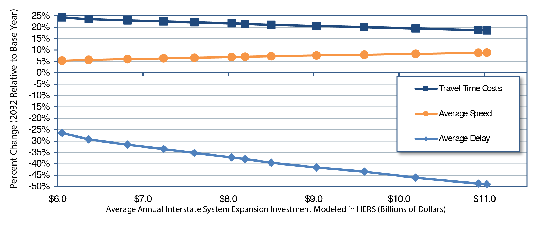
HERS-Modeled Investment on Interstate Highways	Projected 2032 Performance Measures on Interstate Highways				Link to Chapter 8 Scenario
Average Annual for System Expansion (Billions of 2012 Dollars)¹	Average Speed (mph)	percent Change Relative to Baseline
	Average Speed (mph)	Average Speed	Average Delay per VMT	Travel Time Costs per VMT²
$11.0	67.1	8.9%	-49.0%	18.7%	Improve C&P
$10.9	67.1	8.8%	-48.7%	18.8%
$9.6	66.5	8.0%	-43.4%	20.1%
$8.5	66.2	7.3%	-39.5%	21.1%
$8.2	66.0	7.1%	-37.9%	21.5%	Maintain C&P
$7.6	65.7	6.6%	-35.2%	22.2%
$6.8	65.4	6.1%	-31.6%	23.1%	2012 Spending
$6.1	64.9	5.3%	-26.4%	24.3%
Base Year Values:	61.6
¹ The amounts shown represent only the portion of HERS-modeled spending directed toward system expansion, rather than system rehabilitation. Other types of spending can affect these indicators as well. ² Travel time costs are affected by an assumption that the value of time will increase by 1.2 percent in real terms each year; hence, costs would rise even if travel time remained constant. Source: Highway Economic Requirements System; Highway Statistics 2013, Table VM-1.

Impact of Future Investment on Interstate Pavement Ride Quality

Exhibit 7-14 shows the sub-portions of modeled Interstate System spending that HERS allocates to rehabilitation projects (which influence average pavement quality more than expansion projects do). The projected average pavement roughness of NHS roads is sensitive to the level of investment on Interstate System roads. At the highest level of investment presented in Exhibit 714 (an annual average of $12.7 billion allocated to system rehabilitation), the model projects average pavement roughness on the Interstate System to be 9.3 percent lower in 2032 than in 2012. At the lowest level of investment presented in Exhibit 7-14 (an annual average of $7.6 billion allocated to system rehabilitation), the model projects average pavement roughness on the Interstate System to be 11.4 percent higher in 2032 than in 2012.

Exhibit 7-14 Projected 2032 Pavement Ride Quality Indicators on the Interstate System Compared with 2012 for Different Possible Funding Levels

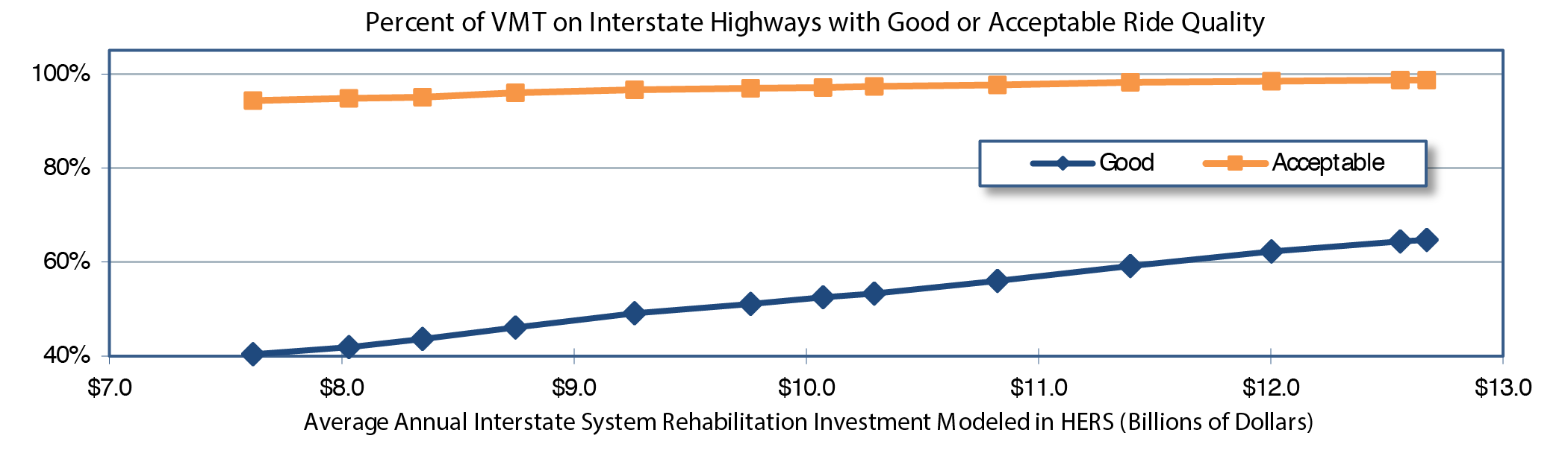
HERS-Modeled Investment on Interstate Highways	Projected 2032 Condition Measures Interstate Highways¹				Link to Chapter 8 Scenario
Average Annual for System Rehabilitation (Billions of 2012 Dollars)²	percent of VMT on Roads with Ride Quality of:		Average IRI (VMT-Weighted)
	Good (IRI<95)	Acceptable (IRI<=170)	Inches Per Mile	Change Relative to Base Year
$12.7	64.7%	98.7%	85.6	-9.3%	Improve C&P
$12.6	64.4%	98.7%	85.8	-9.1%
$11.4	59.1%	98.2%	89.4	-5.3%
$10.3	53.3%	97.3%	93.6	-0.8%
$10.1	52.5%	97.1%	94.4	0.0%	Maintain C&P
$9.3	49.1%	96.6%	97.2	3.0%
$8.3	43.7%	95.1%	101.9	7.9%	2012 Spending
$7.6	40.4%	94.3%	105.2	11.4%
Base Year Values:	66.8%	95.2%	94.4
¹ As discussed in Chapter 3, IRI values of 95 and 170 inches per mile, respectively, are the thresholds associated with "good" and "acceptable" pavement ride quality on the NHS. ² The amounts shown represent only the portion of HERS-modeled spending directed toward system rehabilitation, rather than system expansion. Other types of spending can affect these indicators as well. Source: Highway Economic Requirements System.

Across all investment levels presented in Exhibit 7-14, the model projects that the share of pavements with an IRI below 95, which was the criterion in Chapter 3 for rating ride quality as "good," would be below the corresponding share in 2012 (66.8 percent ). The share of VMT on Interstate highways with an IRI below 95 in 2032 is highly sensitive to investment levels. At the highest level of investment presented in Exhibit 7-14, 64.7 percent of VMT on Interstate highways is projected to be on roads with an IRI below 95 (a decrease of 2.1 percentage points relative to the base year). At the lowest level of investment presented in Exhibit 7-14, 40.4 percent of VMT on Interstate highways is projected to be on roads with an IRI below 95 (a decrease of 26.4 percentage points relative to the base year).

The share of Interstate pavements with an IRI at or below 170, which was the criterion in Chapter 3 for rating ride quality as "acceptable," is projected to increase from the corresponding share in 2012 (95.2 percent ) at the highest level of investment presented in Exhibit 7-14 (98.7 percent ). At the lowest level of investment, the share of Interstate pavements with an IRI at or below 170 is slightly below the 2012 level (94.3 percent ).

Based on these modeling results, additional investment to increase the percentage of VMT on Interstate highways with "good" quality would be economically inefficient, as the costs would exceed the benefits; however, increasing the percentage of VMT on Interstate highways with "acceptable" ride quality is warranted. A key factor leading to this result is that some improvements are not cost-beneficial until IRI rises above 170 (or even higher). Thus, the HERS analysis tended to focus on improving Interstate roads to reach or maintain "acceptable" status, while forgoing non-cost-beneficial improvements that would achieve or maintain "good" ride quality on some roads.

A related limiting factor is that the Interstate-wide average road quality in the base year is relatively high, with an average IRI below 95, and with 95.2 percent of Interstate roads at "acceptable" road quality. Thus, not only is the model constrained by a relatively small subset of roads for which surface rehabilitation would be cost-beneficial, but also the model confirms that allocating funding to alternative projects can be optimal, provided Interstate pavement quality remains at or near "acceptable" on unimproved surfaces.

National Bridge Investment Analysis System

The scenario estimates relating to bridge repair and replacement shown in this report are derived primarily from NBIAS. NBIAS can synthesize element-level data from the general condition ratings reported for individual bridges in the NBI. The analyses presented in this report are based on synthesized element-level data. Examples of bridge elements include the bridge deck, a steel girder used for supporting the deck, a concrete pier cap on which girders are placed, a concrete column used for supporting the pier cap, or a bridge railing.

NBIAS uses a probabilistic approach to model bridge deterioration for each synthesized bridge element. It relies on a set of transition probabilities to project the likelihood that an element will deteriorate from one condition state to another over a given period. This information, along with details on the cost of maintenance, repair and rehabilitation (MR&R) actions, is used to predict lifecycle costs of maintaining existing bridges, and to develop MR&R policies specifying what MR&R action to perform based on the existing condition of a bridge element. Another key input to the model is the overall objective assumed for MR&R policies. The State of Good Repair strategy, although the most aggressive of the available MR&R policies, generates results more consistent with agency practices and recent trends in bridge conditions compared to the other three strategies evaluated (see Appendix B). Therefore, the State of Good Repair strategy has been adopted for use in the baseline analyses presented in this chapter and in Chapter 8.

The State of Good Repair strategy aims to improve all bridges to good condition that can be sustained through ongoing investment. MR&R investment is front loaded under the State of Good Repair strategy, as large MR&R investments are required in the early years of the forecast period to improve bridge conditions, while smaller MR&R investments are needed in the later years to sustain bridge conditions. Replacement of a bridge is recommended if a bridge evaluation results in lower life-cycle costs as compared to the recommended MR&R work.

To estimate functional improvement needs, NBIAS applies a set of improvement standards and costs to each bridge in the NBI. The system then identifies potential improvements-such as widening existing bridge lanes, raising bridges to increase vertical clearances, and strengthening bridges to increase load-carrying capacity-and evaluates their potential benefits and costs. NBIAS evaluates potential bridge replacements by comparing their benefits and costs with what could be achieved through MR&R work alone. Appendix B discusses NBIAS in detail.

In using NBIAS to project conditions and performance of the Nation's bridges over 20 years, this section considers the alternatives of continuing to invest in bridge rehabilitation at the 2012 level (in constant dollars) and at higher or lower levels. The expenditures modeled pertain only to bridge system rehabilitation; expenditures associated with bridge system expansion are modeled separately as part of the capacity expansion analysis in HERS. (The NBIAS-modeled investments presented here should be considered as additive to the HERS-modeled investments presented above; each capital investment scenario presented in Chapter 8 combines one HERS analysis with one NBIAS analysis and makes adjustments to account for non-modeled spending.)

Performance Measures

NBIAS incorporates engineering criteria to evaluate bridge deficiencies at the level of individual bridge elements, and computes an initial value for the cost of a set of corrective actions that would address all such element-level deficiencies. NBIAS projects the deterioration of the individual bridge elements for future years, which determines the timing, type, and cost of any needed future corrective actions. Of note is that these corrective actions are not limited to bridges rated as structurally deficient or functionally obsolete (see Chapter 3). Instead, the model considers potential actions on all bridges, which allows the software to address element-level deficiencies before they trigger a deficiency rating for the overall bridge (i.e., the bridge as a whole is classified as structurally deficient), consistent with sound principles of asset management.

Most previous editions of the C&P report used the economic bridge investment backlog as the sole indicator of bridge system performance. For this edition of the C&P report, four metrics are presented to provide a more comprehensive view of bridge performance:

Percentage Structurally Deficient by Deck Area
Total Percentage Deficient by Deck Area (used in computing the Maintain Conditions and Performance scenario in Chapter 8)
Average Health Index
Economic Investment Backlog (used in computing the Improve Conditions and Performance scenario in Chapter 8)

The percent Structurally Deficient by Deck Area metric indicates the amount of deck area on bridges classified as structurally deficient. Total percent Deficient by Deck Area metric is the amount of deck area on bridges classified as structurally deficient and functionally obsolete. The Health Index metric is a ranking system (0—100) for bridge elements typically used in the context of decision-making for bridge preventive maintenance. Although the condition state of a bridge element is categorical, it is useful to consider an element's condition at a given time as a point along a continuous timeline with 100 percent in the best state to 0 percent in the worst state. The Health Index merely indicates where the element is along this continuum.

Why are functionally obsolete bridges not represented as separate items in the exhibits in this chapter?

Although included in the total deficient bridge figures, functionally obsolete bridges are intentionally not featured in the exhibits; NBIAS can model some improvements that address functional obsolescence, but it currently does not consider replacing bridges with wider bridges having more through lanes (these types of capacity expansions are instead modeled in HERS). Under this limitation, the percentage of functional obsolete bridges in NBIAS might not consistently decrease as investment increases. As discussed in Chapter 3, if a bridge is both structurally deficient and functionally obsolete, it is classified as structurally deficient. Hence, at higher levels of investment, NBIAS might address structural deficiencies but be unable to address functional obsolescence, causing the percentage of functionally obsolete bridges to increase.

To aggregate the element-level result to the bridge level (i.e., assign a value for the Health Index), a weight is assigned to each element according to the economic consequences of its failure, and then an average of all the weighted elements is calculated. Thus, an element for which a failure has relatively little economic effect, such as a railing, would receive less weight than an element for which a failure might result in closing the bridge, such as a girder. In general, the lower the Health Index is, the higher the priority for rehabilitation or maintenance of the structure, although other factors also are instrumental in determining priority of work on bridges.

The Economic Investment Backlog metric represents the combined cost of all corrective actions for which NBIAS estimates implementation would be cost-beneficial. Consistent with the HERS analysis, implementing all cost-beneficial corrective actions in NBIAS would not necessarily mean that no structurally deficient or functionally obsolete bridges would remain; rather, implementing all cost-beneficial corrective actions in NBIAS would indicate that it would not be cost-beneficial to take any further corrective actions. As noted above, these actions extend to all bridges, not just those rated as structurally deficient or functionally obsolete.

Impacts of Systemwide Investments Modeled by NBIAS

As referenced in Chapter 6, of the $105.2 billion invested in highways in 2012, $16.4 billion was used for bridge system rehabilitation. For investments of the types modeled by NBIAS, Exhibit 715 shows how the total amount invested over the 20-year analysis period influences the bridge performance levels projected for the final year, 2032. If spending were sustained at its 2012 level in constant dollar terms ($16.4 billion, the investment level feeding the Sustain 2012 Spending scenario presented in Chapter 8), projected performance for 2032 would improve relative to 2012 for each performance measure considered. The share of bridges classified as structurally deficient, weighted by deck area, would decrease from 8.2 percent to 2.9 percent . The average Health Index would rise from 92.0 to 95.1. The Economic Investment Backlog would decrease by 83.5 percent relative to its 2012 level of $123.1 billion.

Exhibit 7-15 Projected Impact of Alternative Investment Levels on 2032 Bridge Condition Indicators for All Bridges

A line graph plots values for percent of deck area on bridges classified as structurally deficient over average annual investment in billions of year 2012 dollars modeled in NBIAS for 2012 and 2032. While the line for 2012 structurally deficient bridges remains slightly over 8.0 percent from $12.2 billion to $24.6 billion, the plot for 2032 structurally deficient bridges has an initial value of 7.0 percent at an annual investment of $12.2 billion and curves smoothly downward to a value of 3.8 percent at an annual investment of $14.8 billion. Continuing downward, the plot reaches a value of 2.6 percent at an annual investment of $18.2 billion, ending at a value of 1.9 percent at an annual investment of $24.6 billion. Source: National Bridge Investment Analysis System.

NBIAS-Modeled Investment on All Bridges		Projected 2032 Condition Indicators-All Bridges				Link to Chapter 8 Scenario
Average Annual Investment ¹ (Billions of 2012 Dollars)	Average Annual percent Change vs. 2012	percent Structurally Deficient By Deck Area	Total percent Deficient By Deck Area	Health Index	Economic Investment Backlog¹ (Billions of 2012 Dollars)	Link to Chapter 8 Scenario
$24.6	3.72%	1.9%	21.2%	95.4	$0.0	Improve C&P
$22.7	3.00%	2.2%	21.7%	95.3	$5.5
$20.3	2.00%	2.4%	22.0%	95.2	$10.3
$18.2	1.00%	2.6%	22.4%	95.2	$15.0
$16.4	0.00%	2.9%	22.9%	95.1	$20.3	2012 Spending
$14.8	-1.00%	3.8%	23.9%	94.7	$32.9
$13.4	-2.00%	5.3%	25.2%	94.1	$50.5
$12.2	-2.95%	7.0%	26.7%	93.4	$67.6	Maintain C&P
2012 Baseline Values:		8.2%	26.7%	92.0	$123.1
¹ The amounts shown do not reflect system expansion needs; the bridge components of such needs are addressed as part of the HERS model analysis. Source: National Bridge Investment Analysis System.

The highest level of spending shown in Exhibit 7-15 averages $24.6 billion per year (this feeds the Improve Conditions and Performance scenario in Chapter 8). This level of investment is projected to reduce the percent Structurally Deficient by Deck Area to 1.9 percent and to eliminate the Economic Investment Backlog for bridges by 2032. This indicates that the model does not find that completely eliminating structural deficiencies would be cost-beneficial at any single point in time. In some cases, the model recommends that corrective actions be deferred and, in other cases, estimates that the benefits of replacing a bridge would be outweighed by its costs (suggesting that it should eventually be closed, diverting traffic to other available crossings).

Exhibit 7-15 also indicates that the average annual bridge investment could be reduced from the 2012 level while maintaining bridge performance. An average annual spending decline of 2.95 percent to an average annual investment level of $12.2 billion would still be sufficient to maintain the Total percent Deficient by Deck Area at its 2012 level through 2032. At this level of investment, the deck area-weighted share of bridges classified as structurally deficient is projected to drop (improve), the average Health Index is projected to rise (improve), and the Economic Investment Backlog is projected to shrink (improve).

Why does the economic backlog estimated by NBIAS differ from bridge backlog figures estimated by some other organizations?

One major reason for such differences is that the backlog estimated by NBIAS is not intended to constitute a complete bridge investment estimate backlog. The NBIAS figures relate only to investment needs associated with the condition of existing structures, and not capacity expansion needs. The backlog HERS estimates includes estimates of capacity-related needs for highways and bridges combined.

Some estimates of bridge backlog produced by other organizations do attempt to combine estimates of needs relating to bridge capacity with those relating to existing structures.

Impacts of Federal-Aid Highway Investments Modeled by NBIAS

For bridges on Federal-aid highways, Exhibit 7-16 compares performance projections for 2032 at various levels of investment with measured performance in 2012. If spending on the types of improvements modeled in NBIAS were sustained at the 2012 level of $12.0 billion (in constant dollars), performance is projected to improve. The percent Structurally Deficient by Deck Area would decrease from 7.5 percent to 3.3 percent and the average Health Index would rise from 92.0 to 94.8. The Economic Investment Backlog would decrease by 73.4 percent from its 2012 level of $105.8 billion.

If spending declined by 1.77 percent per year to an average annual investment level of $10.0 billion, NBIAS projects Total percent Deficient by Deck Area would be the same in 2032 as in 2012. The remaining metrics would improve with the Economic Investment Backlog showing the largest change from its 2012 level, a reduction of 47.2 percent by 2032. If spending increased by 4.39 percent per year to an average annual level of $19.5 billion, the Economic Investment Backlog would fall to zero by 2032.

Exhibit 7-16 Projected Impact of Alternative Investment Levels on 2032 Bridge Condition Indicators for Bridges on Federal-Aid Highways

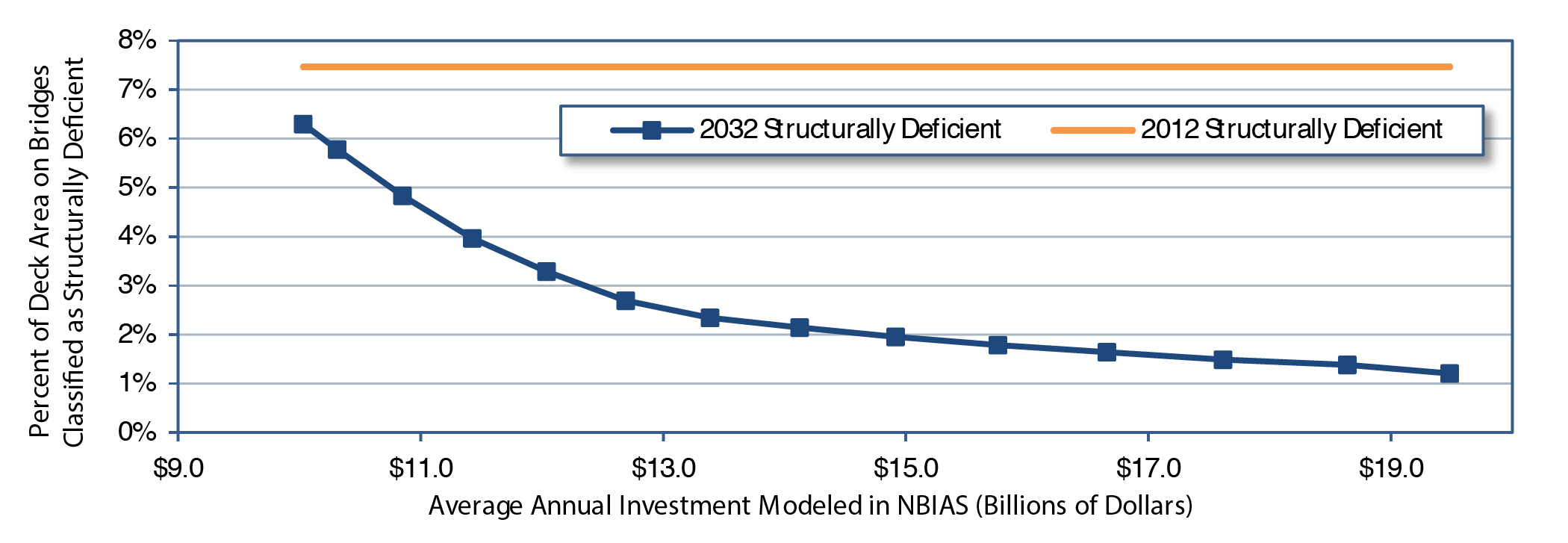
NBIAS-Modeled Investment On Federal-Aid Bridges		Projected 2032 Condition Indicators Bridges on Federal-Aid Highways				Link to Chapter 8 Scenario
Average Annual Investment¹ (Billions of 2012 Dollars)	Average Annual percent Change vs. 2012	percent Structurally Deficient By Deck Area	Total percent Deficient By Deck Area	Health Index	Economic Investment Backlog¹ (Billions of 2012 Dollars)	Link to Chapter 8 Scenario
$19.5	4.39%	1.2%	21.1%	95.4	$0.0	Improve C&P
$18.6	4.00%	1.4%	21.4%	95.4	$2.8
$16.7	3.00%	1.6%	21.8%	95.3	$7.0
$14.9	2.00%	2.0%	22.3%	95.2	$12.4
$13.4	1.00%	2.3%	22.9%	95.2	$17.2
$12.0	0.00%	3.3%	24.0%	94.8	$28.1	2012 Spending
$10.8	-1.00%	4.8%	25.4%	94.2	$43.5
$10.0	-1.77%	6.3%	26.6%	93.5	$55.9	Maintain C&P
2012 Baseline Values:		7.5%	26.6%	92.0	$105.8
¹ The amounts shown do not reflect system expansion needs; the bridge components of such needs are addressed as part of the HERS model analysis. Source: National Bridge Investment Analysis System.

Impacts of NHS Investments Modeled by NBIAS

The impact of various funding levels on the performance of the bridges on the NHS is shown in Exhibit 7-17. If spending on types of improvements modeled in NBIAS on NHS bridges were sustained at the 2012 level of $8.3 billion in constant dollar terms, projected performance for 2032, as measured by the level of Total percent Deficient by Deck Area, would decrease from 26.9 percent to 25.4 percent . The percent Structurally Deficient by Deck Area would decrease from 7.1 percent to 3.1 percent , the average Health Index would increase from 92.0 to 94.9, and the Economic Investment Backlog would decrease by 74.3 percent .

Exhibit 7-17 Projected Impact of Alternative Investment Levels on 2032 Bridge Condition Indicators for Bridges on the National Highway System

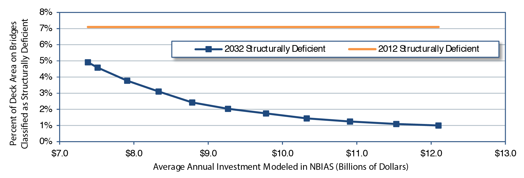
NBIAS-Modeled Investment on NHS Bridges		Projected 2032 Condition Indicators-NHS Bridges				Link to Chapter 8 Scenario
Average Annual Investment¹ (Billions of 2012 Dollars)	Average Annual percent Change vs. 2012	percent Structurally Deficient By Deck Area	Total percent Deficient By Deck Area	Health Index	Economic Investment Backlog¹ (Billions of 2012 Dollars)	Link to Chapter 8 Scenario
$12.1	3.43%	1.0%	23.1%	95.5	$0.0	Improve C&P
$11.5	3.00%	1.1%	23.2%	95.4	$1.4
$10.3	2.00%	1.4%	23.7%	95.4	$5.4
$9.3	1.00%	2.0%	24.4%	95.3	$10.2
$8.3	0.00%	3.1%	25.4%	94.9	$19.1	2012 Spending
$7.5	-1.00%	4.6%	26.6%	94.3	$30.8
$7.4	-1.17%	4.9%	26.9%	94.1	$32.7	Maintain C&P
2012 Baseline Values:		7.1%	26.9%	92.0	$74.2
¹ The amounts shown do not reflect system expansion needs; the bridge components of such needs are addressed as part of the HERS model analysis. Source: National Bridge Investment Analysis System.

A 3.43-percent annual increase in spending to an average annual investment level of $12.1 billion would reduce the Economic Investment Backlog to zero by 2032. The percent Structurally Deficient by Deck Area would decrease to 1.0 percent from 7.1 percent in 2012. The Total percent Deficient by Deck Area would decrease from 26.9 in 2012 to 23.1 percent in 2032 and the average Health Index would increase from 92.0 to 95.5 during the same period. A decline in spending by 1.17 percent per year to an average annual investment level of $7.4 billion would reduce the Economic Investment Backlog in 2032 by 55.9 percent from the level in 2012 (from $74.2 billion to $32.7 billion).

Impacts of Interstate Investments Modeled by NBIAS

Exhibit 7-18 shows the impact of varying funding levels on the performance of bridges on the Interstate System. If spending on types of improvements modeled in NBIAS on Interstate bridges were sustained at the 2012 level of $3.8 billion in constant dollar terms, the Total percent Deficient by Deck Area would increase from 28.5 percent to 29.2 percent by 2032. Projected performance for 2032 would improve for the other metrics relative to 2012: the percent Structurally Deficient by Deck Area would decrease from 7.1 percent in 2012 to 6.6 percent in 2032; the average Health Index would rise from 91.6 to 93.6; and the Economic Investment Backlog would decrease by 44.5 percent to $22.3 billion relative to the 2012 level of $40.2 billion.

Exhibit 7-18 Projected Impact of Alternative Investment Levels on 2032 Bridge Condition Indicators for Interstate Bridges

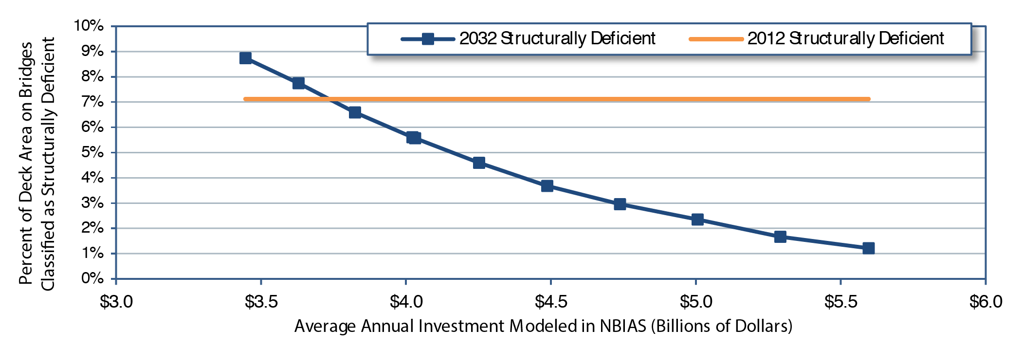
NBIAS-Modeled Investment On Interstate Bridges		Projected 2032 Condition Indicators - Interstate Bridges				Link to Chapter 8 Scenario
Average Annual Investment¹ (Billions of 2012 Dollars)	Average Annual percent Change vs. 2012	percent Structurally Deficient By Deck Area	Total percent Deficient By Deck Area	Health Index	Economic Investment Backlog¹ (Billions of 2012 Dollars)	Link to Chapter 8 Scenario
$5.8	3.77%	1.0%	24.7%	95.4	$0.0	Improve C&P
$5.3	3.00%	1.7%	25.4%	95.3	$3.1
$4.7	2.00%	3.0%	26.7%	95.1	$7.9
$4.3	1.00%	4.6%	27.7%	94.4	$15.1
$4.0	0.48%	5.6%	28.5%	94.0	$18.9	Maintain C&P
$3.8	0.00%	6.6%	29.2%	93.6	$22.3	2012 Spending
$3.4	-1.00%	8.7%	31.0%	92.6	$28.8
2012 Baseline Values:		7.1%	28.5%	91.6	$40.2
¹ The amounts shown do not reflect system expansion needs; the bridge components of such needs are addressed as part of the HERS model analysis. Source: National Bridge Investment Analysis System.

A spending increase of 3.77 percent per year to an average annual level of $5.8 billion is estimated to be sufficient to reduce the Economic Investment Backlog to zero by 2032, decrease the percent Structurally Deficient by Deck Area to 1.0 percent , increase the average Health Index to 95.4, and reduce the Total percent Deficient by Deck Area to 24.7 percent .

Potential Transit Capital Investment Impacts

This section examines how different types and levels of annual capital investments would likely affect transit system condition and performance by 2032. It begins with an overview of the types of capital spending projected by the Federal Transit Administration's (FTA's) Transit Economic Requirements Model (TERM), the primary analysis tool used to assess transit investment needs and impacts in Part II of this report. The section then examines how variations in the level of annual capital spending are likely to affect future transit conditions and performance-both at the national level and for urbanized areas (UZAs) with populations greater than 1 million.

Types of Capital Spending Projected by TERM

TERM is an analysis tool that uses algorithms based on engineering and economic concepts to forecast total capital investment needs for the U.S. transit industry through a 20-year time horizon. Specifically, TERM is designed to forecast the following types of investment needs:

Preservation: The level of investment in the rehabilitation and replacement of existing transit capital assets required to attain specific investment goals (e.g., to attain a state of good repair [SGR]) subject to potentially limited capital funding.
Expansion: The level of investment in the expansion of transit fleets, facilities, and rail networks required to support projected growth in transit demand (i.e., to maintain performance at current levels as demand for service increases).

TERM includes a benefit-cost test that is applied to expansion scenarios to determine which investments are cost effective and which are not. TERM reports investment costs only for investments that pass the test. The SGR Benchmark, described in Chapter 8, uses a zero-growth assumption and turns off the cost-benefit test. It estimates the cost of maintaining what is currently in service as an analytical exercise and is not considered a realistic scenario.

The data used to support TERM's needs estimates are derived from a variety of sources-including fleet investment and transit performance data obtained from the National Transit Database (NTD), asset inventory data provided by local transit agencies (at FTA's request), and historical rates of ridership growth calculated by region, agency size, and mode. The Low-Growth scenario is 0.5 percent less than the historical trend rate in growth while the High-Growth scenario is 0.5 percent more than the historical trend rate in growth. Appendix C contains a detailed description of the analysis methodology TERM uses, and Chapter 9 provides additional detail on the growth rates.

Preservation Investments

TERM estimates current and future preservation investment needs by first assessing the age and current condition of the Nation's existing stock of transit assets (the results of this analysis were presented in Chapter 3 of this report). TERM then uses this information to assess both current reinvestment needs (i.e., the reinvestment backlog) and the expected level of ongoing investment required to meet the life-cycle needs of the Nation's transit assets over the next 20 years, including all required rehabilitation and replacement activities.

Condition-Based Reinvestment

Rather than relying on age alone in assessing the timing and cost of current and future reinvestment activities, TERM uses a set of empirical asset deterioration curves that estimate asset condition (both current and future) as a function of asset type, age, past rehabilitation activities, and, depending on asset type, past maintenance and utilization levels. An asset's estimated condition at the start of each year over the 20-year forecast horizon determines the timing of specific rehabilitation and replacement activities. Asset condition declines as the asset ages, triggering reinvestment events at different levels of deterioration and ultimately leading to outright replacement.

Financial Constraints, the Investment Backlog, and Future Conditions

TERM is designed to estimate investment needs with or without annual capital funding constraints. When run without funding constraints, TERM estimates the total level of investment required to complete all rehabilitation and replacement needs the model identifies at the time those investment needs come due (hence, with unconstrained analyses after any initial deferred investment is addressed, investment backlog is not appreciable). In contrast, when TERM is run in a financially constrained mode, sufficient funding might not be available to cover the reinvestment needs of all assets. In this case, some reinvestment activities would be deferred until sufficient funds become available. The lack of funds to address all reinvestment needs for some or all of the 20 years of the model forecast results in varying levels of investment backlog during this period. Most analyses presented in this chapter were completed using funding constraints. Similarly, TERM's ability to estimate asset conditions-both current and future-allows for assessment of how future asset conditions are likely to improve or decline given varying levels of capital reinvestment. Finally, note that TERM's benefit-cost analysis is used to determine the order in which reinvestment activities are completed when funding capacity is limited, with investments having the highest benefit-cost ratios addressed first.

Expansion Investments

In addition to ongoing reinvestment in existing assets, most transit agencies also invest in the expansion of their vehicle fleets, maintenance facilities, fixed guideway, and other assets. Investments in expansion assets can be considered as serving two distinct purposes. First, the demand for transit services typically increases over time in line with population growth, employment, and other factors. To maintain current levels of performance in the face of expanding demand, transit operators must similarly expand the capacity of their services (e.g., by increasing the number of vehicles in their fleets). Failure to accommodate this demand would result in increased vehicle crowding, increased dwell times at passenger stops, and decreased operating speeds for existing services. Second, transit operators also invest in expansion projects with the aim of improving current service performance. Such improvements include capital expansion projects (e.g., a new light rail segment) to reduce vehicle crowding or increase average operating speeds. TERM is designed to assess investment needs and impacts for both types of expansion investments.

Expansion Investments: Maintain Performance

To assess the level of investment required to maintain existing service quality, TERM estimates the rate of growth in transit vehicle fleets required to maintain current vehicle occupancy levels given the projected growth rate in transit passenger miles. In addition to assessing the level of investment in new fleet vehicles required to support this growth, TERM also forecasts investments in the expansion of other assets needed to support projected fleet growth, including bus maintenance facilities and, in the case of rail systems, additional investment in guideway, track work, stations, maintenance facilities, train control, and traction power systems. Asset expansion investment needs are assessed on a mode-by-mode basis for all agencies reporting to NTD. Cost-benefit constraints, however, prevent TERM from investing in asset expansion for those agency modes having lower ridership (per vehicle) than the national average.

Expansion Investments: Improve Performance

In previous editions of the C&P report, TERM was used to estimate the level of investment required to improve current transit performance by (1) reducing crowding in higher-utilization transit systems, and (2) expanding existing investment in rail to improve average operating speeds in urbanized areas having average operating speeds (across all transit modes) well below the national average. For this edition, the impact of increased investment on system performance is assessed by developing TERM scenarios where the rate of investment in transit asset expansion exceeds the projected rate of growth in transit passenger miles. This difference between the rate of asset expansion and actual growth in travel demand represents projected long-term reductions in in-vehicle crowding and potential increases in average operating speed.

Recent Investment in Transit Preservation and Expansion

Exhibit 7-19 shows the broad composition of the 2012 spending by U.S. transit agencies on capital projects that correspond to the investment types TERM models. Of the total spending of $17.1 billion, $10.0 billion or 58.5 percent was devoted to preserving existing assets, and the rest was spent on expansion investments.

Exhibit 7-19 2012 Transit Capital Expenditures¹

Stacked bar chart shows distribution of expenditures across two categories of investment for two population groups. For the category preservation investments, urbanized areas with over 1 million in population accounted for $8.7 billion in expenditures, urbanized areas with under 1 million in population accounted for $1.0 billion in expenditures, and rural services accounted for $0.2 billion in expenditures, for a total of approximately $10 billion. For the category expansion investments, urbanized areas with over 1 million in population accounted for $6.6 billion in expenditures and urbanized areas with under 1 million in population accounted for $0.5 billion in expenditures, for a total of $7.1 billion. Source: National Transit Database.

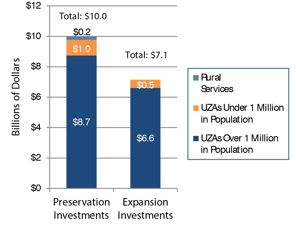
¹Numbers may not sum to total due to rounding.

Source: National Transit Database.

As expected, preservation and expansion spending were concentrated in the large urban systems. In combination, urbanized areas with populations greater than 1 million in 2012 accounted for 87.6 percent of preservation spending and 92.5 percent of expansion spending. Smaller urbanized areas and rural areas accounted for the rest. Although preservation and expansion spending for rural systems is small relative to that for large urban systems, rural transit service has been growing rapidly. Every State and four U.S. Territories provide some form of rural transit service in low-density areas improving the accessibility for Americans living in these areas.

Impacts of Systemwide Investments Modeled by TERM

This section uses TERM analyses to assess how various levels of investment in the preservation and expansion of the Nation's transit asset base can be expected to influence transit conditions and performance over the next 20 years. A key objective here is to place a broad range of potential future investment levels-and the consequences of those levels of investment-within the context of both the current expenditures on transit preservation and expansion and some potential investment goals (e.g., attainment of an SGR within 20 years). More specifically, these analyses consider the impact of different levels of transit capital expenditures on the following:

Preservation Investments-Average condition rating of U.S. transit assets and SGR backlog
Expansion Investments-Additional ridership (boardings) capacity.

Each analysis is completed first at the national level (the remainder of this section) and then repeated (in the following section) for two different segments of urbanized areas, including the following:

Urbanized areas with populations greater than 1 million
All other urbanized areas and rural areas with existing transit services.

Impact of Preservation Investments on Transit Backlog and Conditions

This subsection considers the expected impact of varying levels of aggregate capital reinvestment by all levels of government on the future investment backlog and physical condition (as of 2032) for the Nation's existing stock of transit assets.

Transit Backlog

The 2010 Conditions and Performance Report introduced the concept of reinvestment backlog as an indication of the amount of near-term investment needed to replace assets that are past their expected useful lifetime. Reinvestment backlog focuses attention on assets that are in the worst condition rather than on the average condition of all assets, which is reported below and had been the primary measure in previous editions. This additional perspective is needed because average condition has become less meaningful in the current environment with high levels of investment in new assets for transit system expansion. Investment backlog is a measure of the need for investment in infrastructure preservation. TERM estimates that investment backlog is $89.8 billion (see Chapter 8).

Exhibit 7-20 focuses on the impact of future spending levels on this investment backlog. Specifically, Exhibit 7-20 presents the estimated impact of differing levels of annual capital reinvestment on the expected size of the investment backlog in 2032. Here the investment backlog is defined as the level of investment required to bring all of the Nation's assets to an SGR. This includes replacing those assets that currently exceed their useful lives (the $89.8 billion) and completing all major rehabilitation activities and replacing assets that will exceed their useful lives during the analysis period. If future reinvestment rates are insufficient to address these ongoing reinvestment needs as they arise, the size of the backlog will increase over time. Reinvestment at a rate above that required to address new needs as they arise will ultimately result in elimination of the existing backlog.

As shown in Exhibit 7-20, TERM analysis suggests that the current rate of capital reinvestment of $9.8 billion is insufficient to keep pace with ongoing rehabilitation and replacement needs and, if maintained over the next 20 years, would result in a reinvestment backlog of roughly $122.1 billion by 2032. In contrast, increasing the annual rate of reinvestment to an average of $17.0 billion would eliminate the backlog by 2032. The annual level of reinvestment would need to be increased to roughly $11.4 billion just to maintain the backlog at roughly its current size.

Transit Conditions

Exhibit 7-21 presents the estimated impact of various levels of annual rehabilitation and replacement investments on the average physical condition of all existing assets nationwide as of 2032. The exhibit shows ongoing improvements to the overall condition of the Nation's existing transit asset base from increasing levels of transit capital reinvestment. Of special note is that average condition provides a measure of asset conditions taken together. Hence, even though overall conditions improve with additional expenditures, the condition of some individual assets is expected to continue to deteriorate (given the length of asset lives and the timing of their replacement cycles) while the condition of other assets improves. The value of the aggregate measure lies in providing an overall, single measure of asset conditions. Moreover, given the relationship between asset condition and asset reliability, any general improvement in overall asset conditions also can be associated with related improvements to service quality, reliability, and possibly safety.

Exhibit 7-20 Impact of Preservation Investment on 2032 Transit State of Good Repair Backlog in All Urbanized and Rural Areas

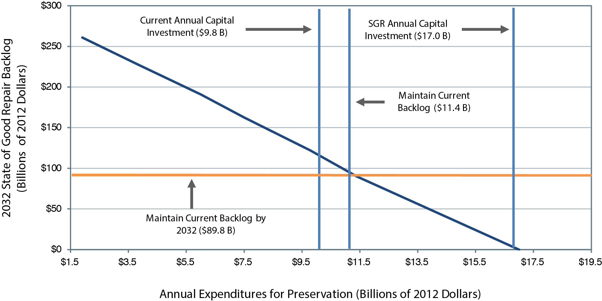
A line chart plots state of good repair backlog in billions of 2012 dollars over annual expenditures for preservation in billions of dollars. The backlog value is approximately $261 billion at an annual expenditure of $1.9 billion. The plot trends steadily downward to backlog of zero at an annual expenditure of $17.0 billion. The plot intersects with the current annual capital investment of $9.8 billion at a backlog value of $122.1 billion, and the current backlog of $89.8 billion is reached at $11.4 billion in annual expenditures. Source: Transit Economic Requirements Model.

Average Annual Investment (Billions of 2012 Dollars)	Average Annual percent Change vs. 2012	Average Condition Rating in 2032¹	Backlog in 2032 (Billions of 2012 Dollars)²	percent Change From Current Backlog	Funding Level Description
$17.0	5.7%	3.20	$0.0	-100%	SGR (unconstrained, replace at 2.50)
$11.4	1.5%	3.17	$89.8	0%	Maintain current backlog
$9.8	0.0%	3.10	$122.1	36%	2012 capital expenditures (sustain 2012 spending)
$7.5	-2.7%	3.03	$162.5	81%	Reduce 2.5 percent ³
$6.0	-5.3%	2.96	$191.1	113%	Reduce 5 percent ³
$3.8	-11.2%	2.86	$228.2	154%	Reduce 10 percent ³
$1.9	-23.7%	2.80	$260.9	191%	Reduce 20 percent ³
¹ For this report, assets are considered past their useful lives once their estimated condition in TERM falls below condition 2.50. ² Data points depicted in the chart might not correspond exactly to data presented in the associated table due to rounding of Average Annual Investment (Billions of 2012 Dollars) amounts. ³ Funding is reduced from current level by the percentage identified every year for 20 years. Source: Transit Economic Requirements Model.

The table portion of Exhibit 7-21 presents the same investment and average condition information as in the chart. This table also presents the impact of reinvestment on asset conditions for five key transit asset categories (i.e., guideway and track, facilities, systems, stations, and vehicles) and the average annual percentage change in constant dollar funding from 2012 levels to achieve each projected condition level.

Exhibit 7-21 Impact of Preservation Investment on 2032 Transit Conditions in All Urbanized and Rural Areas^1,2

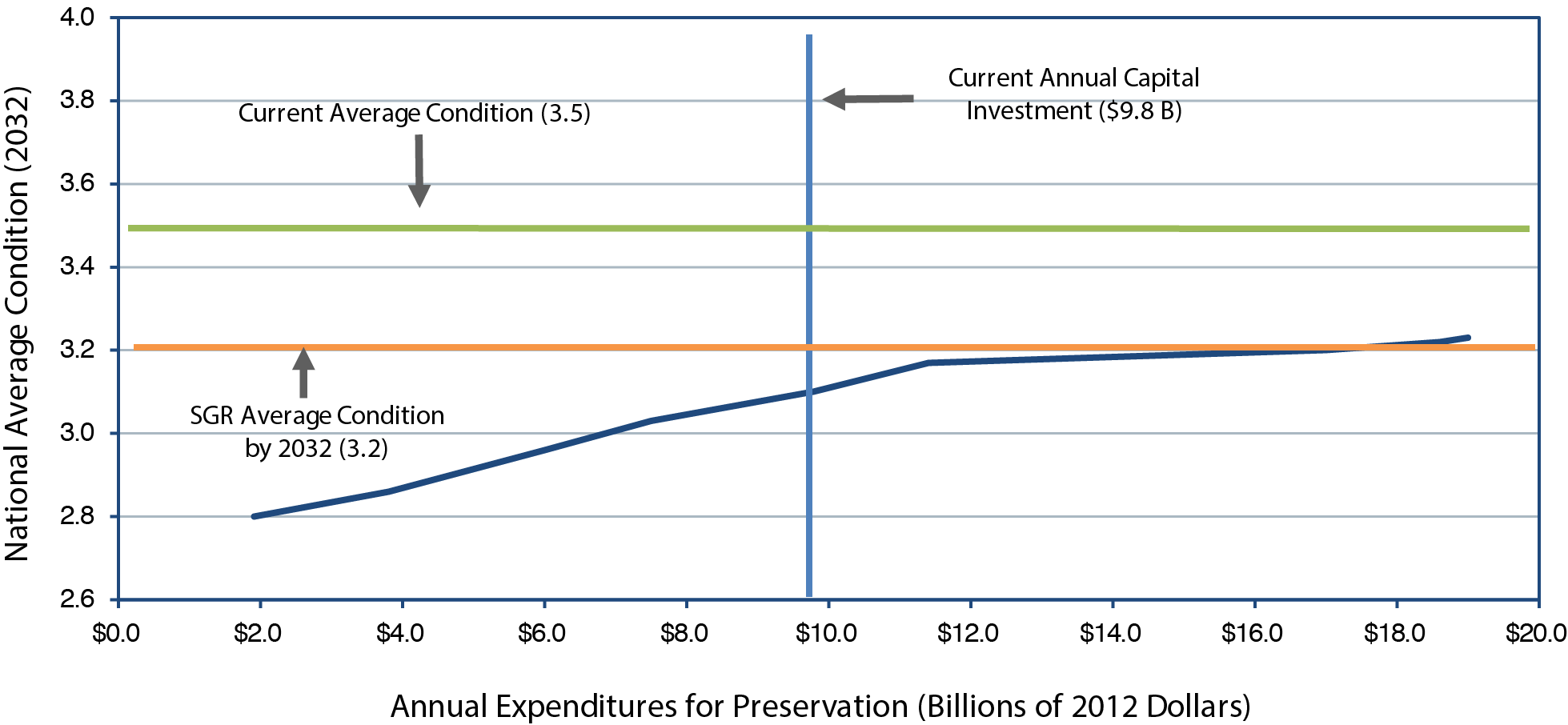
A line chart plots national average condition rating over annual expenditures in billions of dollars. The average transit condition in 2032 has a rating of 2.80 at an annual investment expenditure of $1.9 billion. The plot trends steadily upward to a rating of 3.17 at an annual investment expenditure of $11.4 billion, and continues upward at a slower rate to a rating of 3.23 at an annual expenditure of $19.0 billion. The plot intersects with the rating 3.20 at the current annual capital investment amount of $17.0 billion. The plot ends at a rating value of 3.23, short of the current average condition rating of 3.5, with an expenditure of $19 billion. Source: Transit Economic Requirements Model.

Average Annual Investment (Billions of 2012 Dollars) Total Capital Outlay	Average Annual percent Change vs. 2012	Average Transit Conditions in 2032						Funding Level Description
		Asset Categories					All Transit Assets³
		Guideway	Facilities	Systems	Stations	Vehicles	All Transit Assets³
$19.0	7.8%	2.77	3.19	3.55	3.64	3.38	3.23	Unconstrained, replace at 3.00
$18.6	6.5%	2.76	3.19	3.55	3.64	3.38	3.22	Unconstrained, replace at 2.75
$17.0	5.8%	2.71	3.19	3.55	3.64	3.38	3.20	SGR (unconstrained, replace at 2.50)
$11.4	1.6%	2.67	2.94	3.58	3.63	3.36	3.17	Maintain current backlog
$9.8	0.0%	2.64	2.61	3.48	3.52	3.40	3.10	2012 capital expenditures
$7.5	-2.7%	2.55	2.61	3.35	3.48	3.34	3.03	Reduce 2.5 percent
$6.0	-5.3%	2.49	2.61	3.12	3.46	3.28	2.96	Reduce 5 percent
$3.8	-11.2%	2.44	2.61	2.77	3.45	3.05	2.86	Reduce 10 percent
$1.9	-23.7%	2.40	2.61	2.67	3.45	2.80	2.80	Reduce 20 percent
¹ The conditions of individual transit assets are estimated using TERM's asset decay curves, which estimate asset conditions on a scale of 5 (excellent) through 1 (poor), as described earlier in this chapter and in Appendix C to this report. The average national condition is the weighted average of the condition of all assets nationwide, weighted by the estimated replacement cost of each asset. ² This preservation analysis is intended to consider reinvestment needs only for existing transit assets (as of 2012), not for expansion assets to be added to the existing capital stock in future years. ³ Data points depicted in the chart might not correspond exactly to data presented in the associated table due to rounding of Average Annual Investment (Billions of 2012 Dollars) amounts. Source: Transit Economic Requirements Model.

Further review of Exhibit 7-21 reveals several observations. First, note that none of the selected reinvestment rates presented (including the current level of reinvestment, which was $9.8 billion in 2012) is sufficient to maintain aggregate conditions at or near the current national average condition rating of 3.5. Even the highest reinvestment rate presented here of $19.0 billion annually (replacement at condition rating 3.0), which is an aggressive reinvestment rate, is not sufficient to maintain aggregate conditions at current levels. A primary factor driving this result is the ongoing expansion investment in new rail systems over the past several decades. Although this expansion investment has tended to maintain or even increase the average condition rating of assets nationwide (despite the ongoing deterioration of older assets), it also has resulted in an average condition rating that is not sustainable in the long term (i.e., without including the influence of further expansion investments or replacing assets at an unreasonably early age). Second, note that reinvestment at roughly $17.0 billion annually is required to attain an SGR condition by 2032 and that this level of reinvestment is estimated to yield an average condition value of roughly 3.20 by that year. Given the definition of the SGR Benchmark (described in more detail in Chapter 8), which seeks to eliminate the existing investment backlog and then address all subsequent rehabilitation and replacement activities "on time" thereafter, the 3.20 value could be considered representative of the expected long-term average condition of a well-maintained and financially unconstrained national transit system. Hence, an average condition rating of roughly 3.20 represents a more reasonable long-term condition target for existing transit infrastructure than the current aggregate rating of 3.5.

Another observation is that a significant level of reinvestment is required to alter the estimated 2032 average condition measure by a point or more. This result is also driven in part by a large proportion of transit assets with expected useful lives of 80 years or more that will not require significant reinvestment over the 20-year period of this analysis (regardless of the level of reinvestment). These assets tend to contribute a high weighting in the average condition measure, making the measure somewhat insensitive to the rate of reinvestment (note that a high proportion of reinvestment activity is focused on the replacement of those assets with relatively shorter useful lives, such as vehicles).

Finally, TERM prioritizes asset needs based on five criteria (condition, reliability, safety, riders impacted, and operations and maintenance cost impacts) with condition having the highest weighting. Replacement and rehabilitation investments are both subject to this same prioritization scoring. Replacement needs tend to score higher, however, as they tend to reflect the needs of assets that are in poorer condition than those assets requiring rehabilitation. Therefore, rehabilitation needs tend not to be addressed until most (but far from all) replacement needs are addressed. TERM currently predicts improvement in asset condition only following a replacement. Hence, expenditures past approximately $11.8 billion on the chart increase total cost as rehabilitation projects are added, but these projects do not contribute to an increase in condition ratings.

Expansion Investments and Transit Ridership

Although capital spending on preservation primarily benefits the physical condition of existing transit assets, expansion investments are typically undertaken to expand the asset base to accommodate projected growth in ridership and potentially to improve service performance for existing transit system users.

Exhibit 7-22 shows the relationship between aggregated annual capital spending by all levels of government on expansion investments and the additional number of annual passenger boardings that transit systems would be able to support by 2032. More precisely, this chart presents the level of expansion investment required to ensure that transit vehicle occupancy rates are maintained at current levels over the next two decades for a broad range of the potential rates of growth in transit passenger miles traveled. As the upward sloping curve of the chart indicates, higher levels of investment are required to support greater numbers of additional riders at a constant level of service. If investment levels are insufficient to support the projected growth in ridership fully, vehicle occupancy rates will tend to increase, leading to increased crowding on high-utilization systems and potentially leading to increased dwell times at stops, reduced average operating speeds, and increased rates of vehicle wear. Conversely, if the rate of transit capacity expansion exceeds the actual rate of ridership growth, occupancy rates will tend to decline and service performance would likely improve.

Exhibit 7-22 New Ridership Supported in 2032 by Expansion Investments in All Urbanized and Rural Areas¹

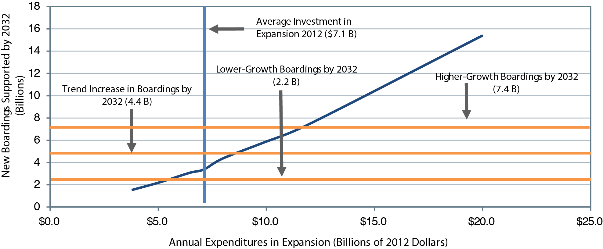
A line chart plots new boardings supported by the year 2032 over annual expenditures in expansion. The plot has an initial value of 1.6 billion new riders supported annually at an annual expenditure of $3.8 billion, and trends upward to a value of 15.4 billion new riders supported annually at an annual expenditure of $20 billion. The plot intersects with the 15-year historic growth rate trend increase of 4.4 billion in boardings by 2032 at an annual expenditure of $8 billion. The current average investment in expansion is $7.1 billion. Source: Transit Economic Requirements Model.

Average Annual Investment (Billions of 2012 Dollars)	Average Annual percent Change vs. 2012	Total New Boardings by 2032		Funding Level Description
Average Annual Investment (Billions of 2012 Dollars)	Average Annual percent Change vs. 2012	New Riders Supported (Billions of Annual Boardings)	Average Annual Growth in Boardings²	Funding Level Description
$20.0	9.3%	15.4	4.6%	Highest-growth scenario (+1.5%)
$11.9	4.9%	7.4	2.7%	Higher-growth scenario (+1.0%)
$9.9	3.2%	5.8	2.2%	High-growth scenario (+0.5%)
$8.0	1.2%	4.4	1.7%	15-year historic growth rate trend
$7.1	0.0%	3.4	1.5%	2012 expansion expenditures
$6.4	-1.0%	3.1	1.3%	Low-growth scenario (-0.5%)
$5.1	-3.5%	2.2	1.0%	Lower-growth scenario (-1.0%)
$3.8	-6.9%	1.6	0.7%	Lowest-growth Scenario (-1.5%)
¹ TERM assesses expansion needs at the agency-mode level subject to (1) current vehicle occupancy rates at the agency-mode level and (2) expected transit PMT growth at the UZA level (hence, all agency modes within a given UZA are subject to the same transit PMT growth rate). Note, however, that TERM does not generate expansion needs estimates for agency modes that have occupancy rates that are well below the national average for that mode. ² As compared with total urban ridership in 2012; only includes increases covered by investments passing TERM's benefit-cost test. Source: Transit Economic Requirements Model.

The findings presented in Exhibit 7-22 suggest the following trends. First, the recent rate of investment in asset expansion ($7.1 billion in 2012) could support roughly 3.4 billion additional boardings by 2032 (approximately a 1.5-percent annual growth in ridership). Assuming that the actual rate of ridership growth is close to the trend rate of growth for the past 15 years, an average capital investment of $8.0 billion annually in transit expansion would be required over the next 20 years to support an additional 4.4 billion annual boardings-again after excluding expansion investments that do not pass TERM's benefit-cost test. Hence, although the existing levels of transit capital expansion investment might be sufficient to maintain current service performance (i.e., vehicle occupancy rates), if ridership growth is relatively low (1 percent average annual growth in boardings), the corresponding average annual level of investment ($5.1 billion) is roughly twothirds of what is required to support a level of ridership growth consistent with that experienced over the most recent 15-year period.

Impacts of Urbanized Area Investments Modeled by TERM

The remainder of this chapter focuses on how different levels of annual capital investment in the U.S. transit infrastructure affect urbanized areas with dissimilar transit investment needs. Specifically, this section explores the impact of capital expenditures by transit agencies sorted into two distinct UZA groupings: (1) the urbanized areas with populations greater than 1 million and (2) all other urbanized and rural areas with existing transit services.

Urbanized Areas Over 1 Million in Population

The Nation's largest urbanized areas own and operate most of the Nation's existing transit assets. These urbanized areas also typically have the highest levels of investment in older rail assets.

In 2012, transit agencies operating in urbanized areas with populations greater than 1 million spent $15.4 billion on capital projects. This expenditure consisted of $8.7 billion on preservation investments intended to rehabilitate or replace existing assets and $6.6 billion on expansion investments designed to increase service capacity. The following is a discussion of the transit asset preservation and expansion needs of these urbanized areas with populations greater than 1 million.

Preservation Investments

As shown in Exhibit 7-23, the 2012 level of capital reinvestment for the largest urbanized areas-$8.7 billion-is insufficient to keep pace with ongoing rehabilitation and replacement needs. Further, maintaining this reinvestment amount over the next 20 years would result in a larger SGR backlog of roughly $120.5 billion by 2032 compared with the current $88.6 billion backlog. In contrast, increasing the rate of reinvestment to an annual average of roughly $15.7 billion would eliminate the entire backlog by 2032. The annual level of reinvestment would need to be increased to roughly $10.2 billion to maintain the backlog at about its current size.

Exhibit 7-23 Impact of Preservation Investment on 2032 Transit State of Good Repair Backlog in Urbanized Areas with Population over 1 Million

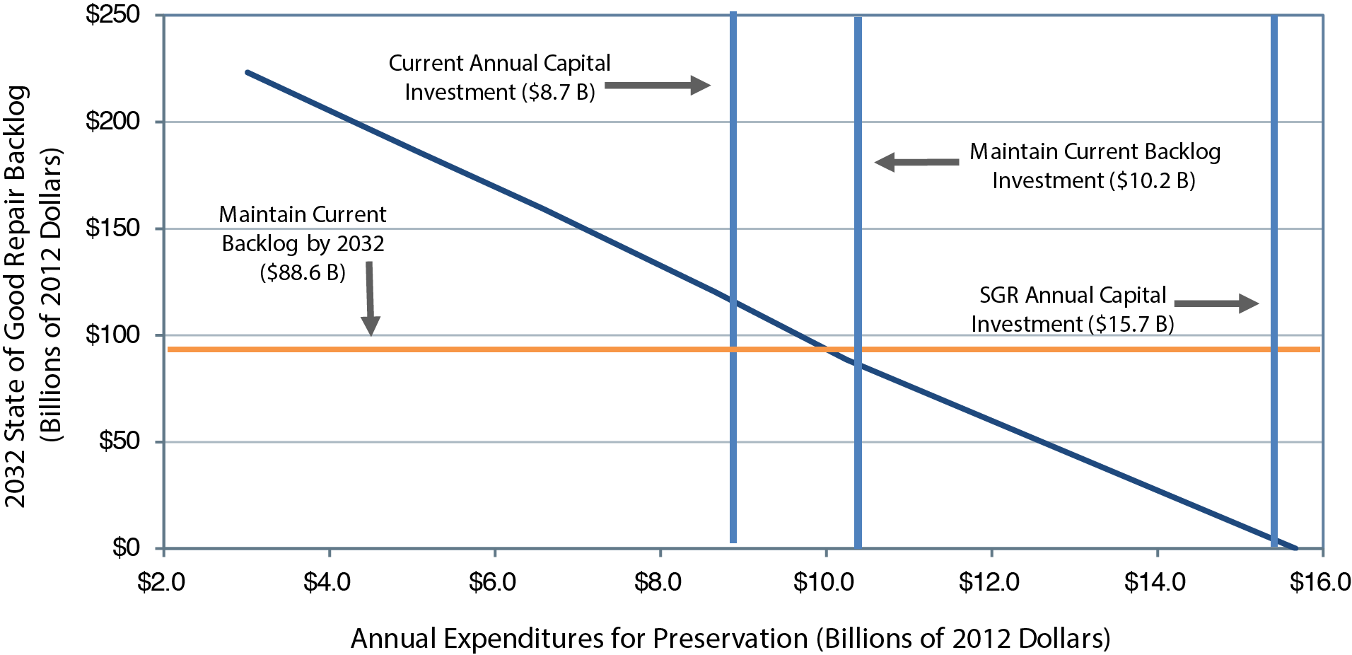
A line chart plots state of good repair backlog over annual expenditures for preservation in billions of 2012 dollars. The backlog value is $223.2 billion at an annual expenditure of $3.0 billion. The plot trends steadily downward to a backlog of zero at an annual expenditure of $15.7 billion. The plot intersects at an annual capital investment of $8.7 billion with a backlog of $120.5 billion, and reaches the current backlog of $88.6 billion with annual expenditures of 10.2 billion. Source: Transit Economic Requirements Model.

Average Annual Investment (Billions of 2012 Dollars)	Average Annual percent Change vs. 2012	Replacement Condition¹	Average Condition Rating in 2032	Backlog in 2032 (Billions of 2012 Dollars)²	Funding Level Description
$15.7	5.5%	2.50	3.19	$0.0	SGR (unconstrained, replace at 2.50)
$10.2	1.6%	2.50	3.16	$88.6	Maintain current backlog
$8.7	0.0%	2.50	3.09	$120.5	2012 capital expenditures (sustain 2012 spending)
$6.6	-2.9%	2.50	3.02	$159.3	Reduce 2.5 percent
$5.0	-6.1%	2.50	2.95	$186.6	Reduce 5 percent
$3.0	-13.1%	2.50	2.85	$223.2	Reduce 10 percent
¹ For this report, assets are considered past their useful lives once their estimated condition in TERM falls below condition 2.50. ² Data points depicted in the chart might not correspond exactly to data presented in the associated table due to rounding of Average Annual Investment (Billions of 2012 Dollars) amounts. Source: Transit Economic Requirements Model.

Exhibit 7-24 shows the estimated impact of varying levels of preservation investments on the future condition of existing transit assets located in urbanized areas with populations greater than 1 million. As was shown in Exhibit 7-21 covering the entire industry, this chart clearly indicates that, due to significant recent investments in long-lived expansion assets, the current average condition rating for transit assets located in the largest urbanized areas is not sustainable in the long term without replacing assets on an aggressive schedule (i.e., replacement at or before condition rating 3.0). At the same time, the 2012 level of reinvestment ($8.7 billion) is less than that required to attain an SGR ($15.7 billion), with the latter supporting a more sustainable long-term average condition rating of roughly 3.19.

Exhibit 7-24 Impact of Level of Preservation Investment on 2032 Transit Conditions in Urbanized Areas with Population over 1 Million^1,2

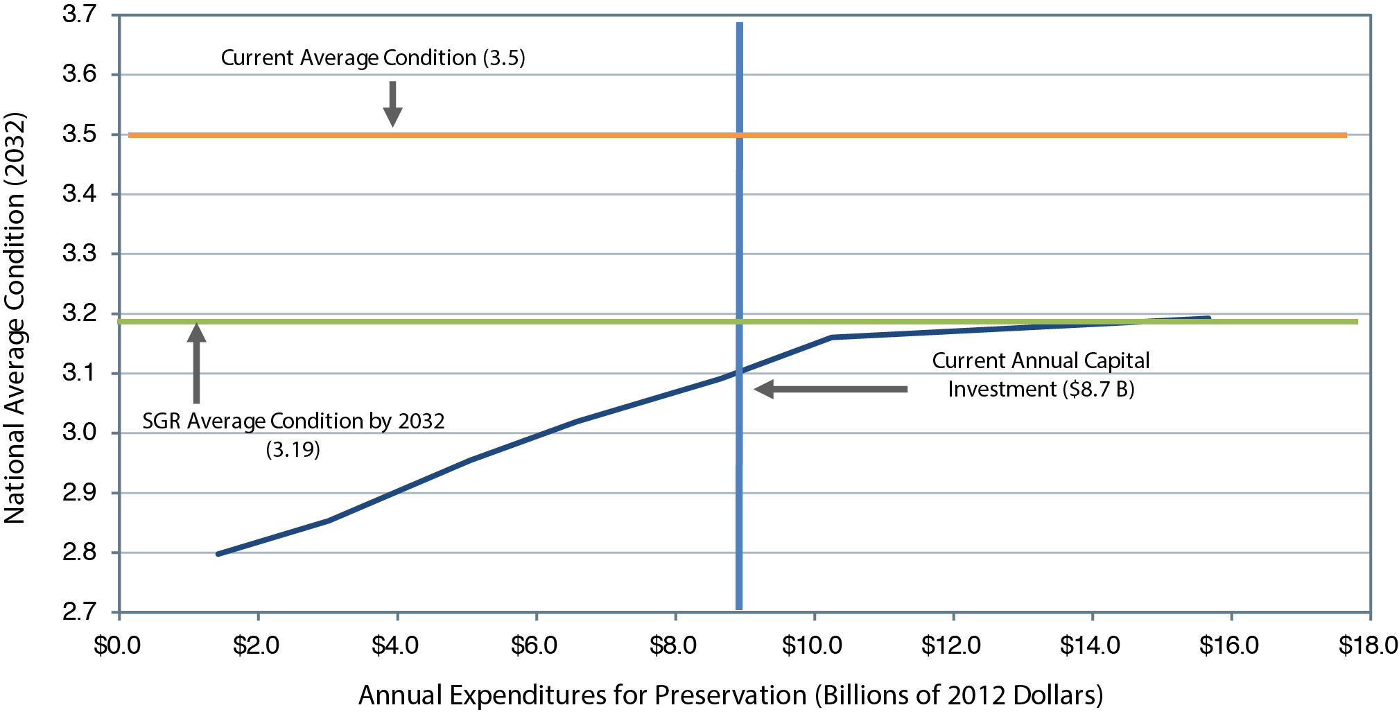
A line chart plots national average condition rating over annual expenditures for preservation in billions of 2012 dollars. The plot has an initial rating of 2.80 at an annual expenditure of $1.4 billion. The trend is steadily upward to a value of 3.16 at an average annual investment of $10.2 billion, and levels off to reach a value of 3.19 at an average annual investment of $15.7 billion. The plot intersects at a rating of 3.09 with the annual current annual capital investment of $8.7 billion. The current average condition is shown as a rating of 3.5, and the SGR average condition by 2032 is shown as a rating of 3.19. Source: Transit Economic Requirements Model.

Average Annual Investment (Billions of 2012 Dollars) Total Capital Outlay	Average Annual percent Change vs. 2012	Average Transit Conditions in 2032						Funding Level Description
		Asset Categories					All Transit Assets³
		Guideway	Facilities	Systems	Stations	Vehicles	All Transit Assets³
$15.7	5.6%	2.68	3.19	3.55	3.64	3.38	3.19	SGR (unconstrained condition, replace at 2.50)
$10.2	1.6%	2.64	2.97	3.58	3.63	3.36	3.16	Maintain current backlog
$8.7	0.0%	2.61	2.62	3.49	3.52	3.39	3.09	2012 capital expenditures (maintain current spending)
$6.6	-2.8%	2.53	2.62	3.36	3.48	3.33	3.02	Reduce 2.5 percent
$5.0	-5.9%	2.47	2.62	3.12	3.46	3.28	2.95	Reduce 5 percent
$3.0	-12.9%	2.42	2.62	2.77	3.45	3.03	2.85	Reduce 10 percent
$1.4	-29.0%	2.38	2.62	2.67	3.45	2.80	2.80	Reduce 20 percent
¹ The conditions of individual transit assets are estimated using TERM's asset decay curves, which estimate asset conditions on a scale of 5 (excellent) through 1 (poor), as described earlier in this chapter and in Appendix C to this report. The average national condition is the weighted average of the condition of all assets nationwide, weighted by the estimated replacement cost of each asset. ² This preservation analysis is intended to consider reinvestment needs only for existing transit assets (as of 2012), not for expansion assets to be added to the existing capital stock in future years. ³ Data points depicted in the chart might not correspond exactly to data presented in the associated table due to rounding of Average Annual Investment (Billions of 2012 Dollars) amounts. Source: Transit Economic Requirements Model.

Expansion Investments

Although urbanized areas with populations greater than 1 million tend to be cities with slower rates of increase in population and transit ridership (e.g., Boston, Philadelphia, and Chicago), this group also includes urbanized areas expected to experience relatively high rates of growth in transit boardings and passenger miles traveled over the next two decades, including Los Angeles, Atlanta, and Seattle. Given the high numbers of existing riders and transit capacity in these higher-growth large urbanized areas, they will require significant increases in expansion investments to maintain current service performance during this period.

Exhibit 7-25 presents estimates of expansion investment level required to support varying levels of growth in transit demand while maintaining current performance levels (as measured by vehicle capacity utilization) for these large urbanized areas. Note that the 2012 level of investment for these urbanized areas ($6.6 billion) was more than that required to support the rate of increase in transit demand as projected by the Low-Growth scenario (0.5 percent below the trend rate of increase as experienced in recent years) but well short of that required to support a high rate of growth (0.5 percent above the trend rate of increase as experienced in recent years).

Other Urbanized and Rural Areas

The following analysis considers the combined preservation and expansion needs of urbanized areas with populations less than 1 million and those of all rural areas with existing transit service. This diverse group therefore includes numerous mid-sized and small urbanized and rural transit operators offering only bus or para-transit services, or both.

In 2012, transit agencies operating outside of the largest urbanized areas spent $1.7 billion on capital projects, with $1.2 billion on preservation intended to rehabilitate or replace existing assets and $0.5 billion on expansion designed to increase service capacity. The following is a discussion of the transit asset preservation and expansion needs of transit agencies in these areas.

Preservation Investments

As shown in Exhibit 7-26, the 2012 level of capital reinvestment of $1.1 billion for rural areas and smaller urbanized areas is insufficient to keep pace with ongoing rehabilitation and replacement needs. If maintained over the next 20 years, this rate of investment would result in a larger SGR backlog of roughly $1.7 billion by 2032, as compared with the current backlog of $1.3 billion for this group. In contrast, increasing the rate of reinvestment to an annual average of roughly $1.3 billion would eliminate the entire backlog by 2032. The annual level of reinvestment would need to be increased to roughly $1.2 billion annually to maintain the backlog at about its current size.

Exhibit 7-25 New Ridership Supported in 2032 by Expansion Investments in Urbanized Areas with Population over 1 Million¹

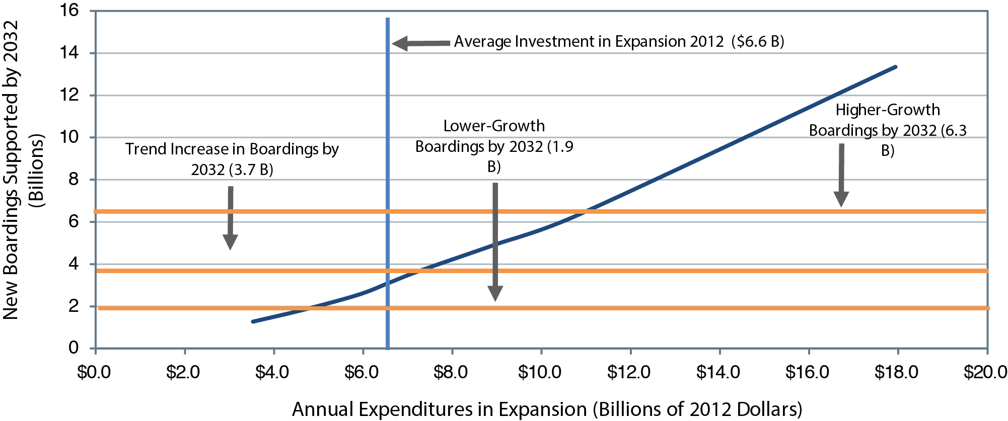
A line chart plots new boardings supported by the year 2032 over annual expenditures in expansion. The plot has an initial value of 1.3 billion new riders supported annually at an annual expenditure of $3.5 billion, and trends upward to a value of 13.3 billion new riders supported annually at an annual expenditure of $17.9 billion. The plot intersects with the trend increase of 3.7 billion in boardings by 2032. The current average investment in expansion is $6.6 billion. Source: Transit Economic Requirements Model.

Average Annual Investment (Billions of 2012 Dollars)	Average Annual percent Change vs. 2012	Total New Boardings by 2032		Funding Level Description
Average Annual Investment (Billions of 2012 Dollars)	Average Annual percent Change vs. 2012	New Riders Supported (Billions of Annual Boardings)²	Average Annual Growth in Boardings³	Funding Level Description
$17.9	9.9%	13.3	4.5%	Highest-growth scenario (+1.5%)
$10.8	5.5%	6.3	2.6%	Higher-growth scenario (+1.0%)
$9.0	3.8%	4.9	2.1%	High-growth scenario (+0.5%)
$7.3	1.9%	3.7	1.7%	15-year historic growth rate trend
$6.6	0.0%	3.1	1.4%	2012 expansion expenditures
$5.9	-0.2%	2.6	1.2%	Low-growth scenario (-0.5%)
$4.7	-2.7%	1.9	0.9%	Lower-growth scenario (-1.0%)
$3.5	-6.0%	1.3	0.6%	Lowest-growth scenario (-1.5%)
¹ TERM assesses expansion needs at the agency-mode level subject to (1) current vehicle occupancy rates at the agency-mode level and (2) expected transit PMT growth at the UZA level (hence, all agency modes within a given UZA are subject to the same transit PMT growth rate). Note, however, that TERM does not generate expansion needs estimates for agency modes that have occupancy rates that are well below the national average for that mode. ² Data points depicted in the chart might not correspond exactly to data presented in the associated table due to rounding of Average Annual Investment (Billions of 2012 Dollars) amounts. ³ As compared with total urban ridership in 2012; only includes increases covered by investments passing TERM's benefit-cost test. Source: Transit Economic Requirements Model.

Exhibit 7-26 Impact of Preservation Investment on 2032 Transit State of Good Repair Backlog in Urbanized Areas with Population under 1 Million and Rural Areas^1,2

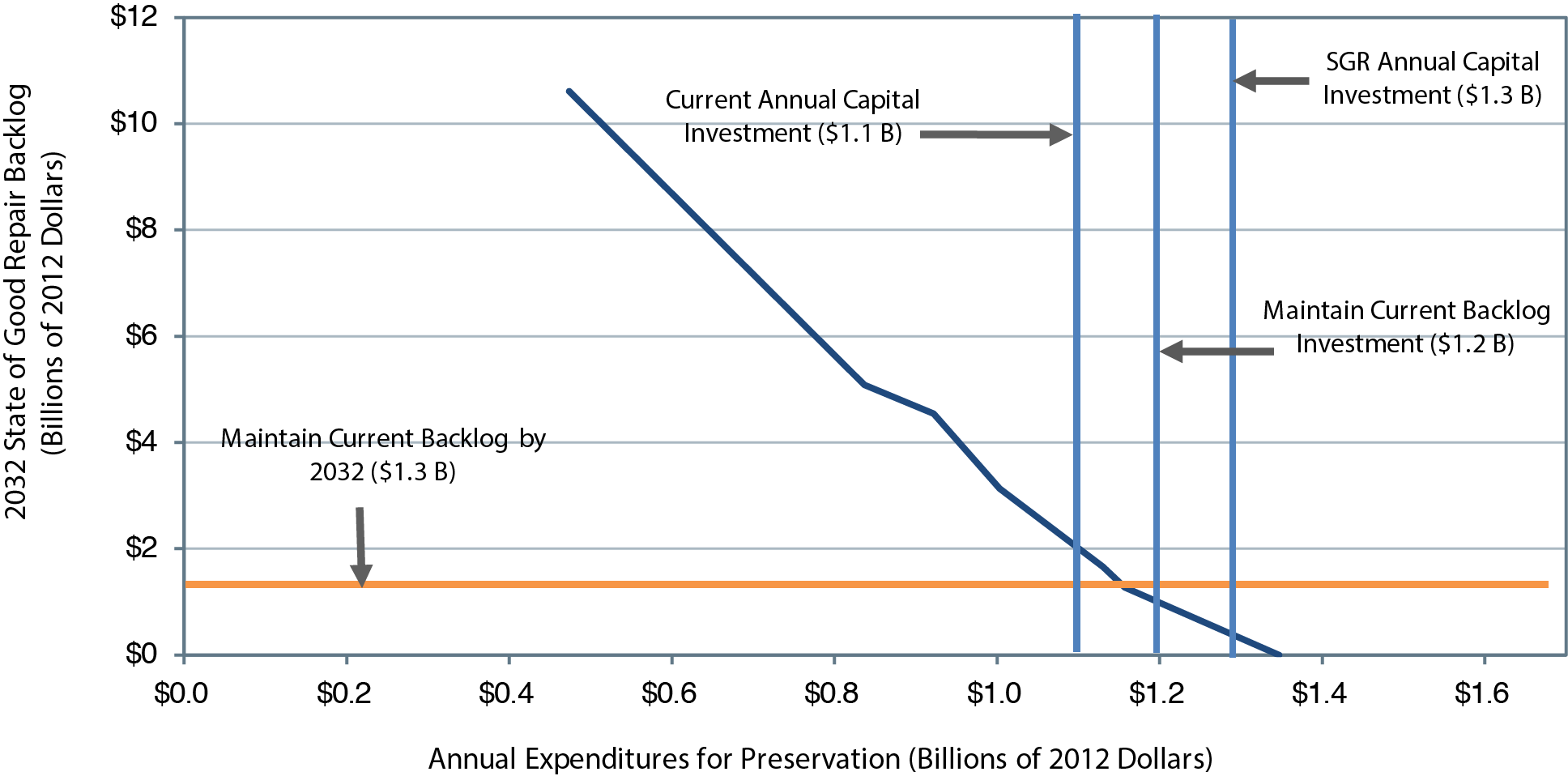
Average Annual Investment (Billions of 2012 Dollars)	Average Annual percent Change vs. 2012	Replacement Condition¹	Average Condition Rating in 2032	Backlog in 2032 (Billions of 2012 Dollars)²	Funding Level Description
$1.3	1.7%	2.50	3.64	$0.0	SGR (unconstrained, replace at 2.50)
$1.2	0.3%	2.50	3.65	$1.3	Maintain current backlog
$1.1	0.0%	2.50	3.63	$1.7	2012 capital expenditures (sustain 2012 spending)
$1.0	-1.2%	2.50	3.44	$3.1	Reduce 2.5 percent
$0.9	-2.1%	2.50	3.33	$4.5	Reduce 5 percent
$0.8	-3.1%	2.50	3.30	$5.1	Reduce 10 percent
$0.5	-10.3%	2.50	3.06	$10.6	Reduce 20 percent
¹ For this report, assets are considered past their useful lives once their estimated condition in TERM falls below condition 2.50. ² Data points depicted in the chart might not correspond exactly to data presented in the associated table due to rounding of Average Annual Investment (Billions of 2012 Dollars) amounts. Source: Transit Economic Requirements Model.

Exhibit 7-27 shows the estimated impact of varying levels of preservation investments on the future condition of existing transit assets located in urbanized areas with populations less than 1 million and in rural areas. As was shown in Exhibit 7-24 for the largest urbanized areas, this chart also indicates that the current average condition rating for transit assets in these smaller urbanized and rural areas is not sustainable in the long term without replacing assets on an aggressive schedule (i.e., replacement at or before condition rating 3.0). At the same time, the 2012 level of reinvestment ($1.1 billion) is less than that required to attain an SGR ($1.3 billion), with the latter supporting a more sustainable long-term average condition rating of roughly 3.63.

Exhibit 7-27 Impact of Preservation Investment on 2032 Transit Conditions in Urbanized Areas with Population under 1 Million and Rural Areas^1,2

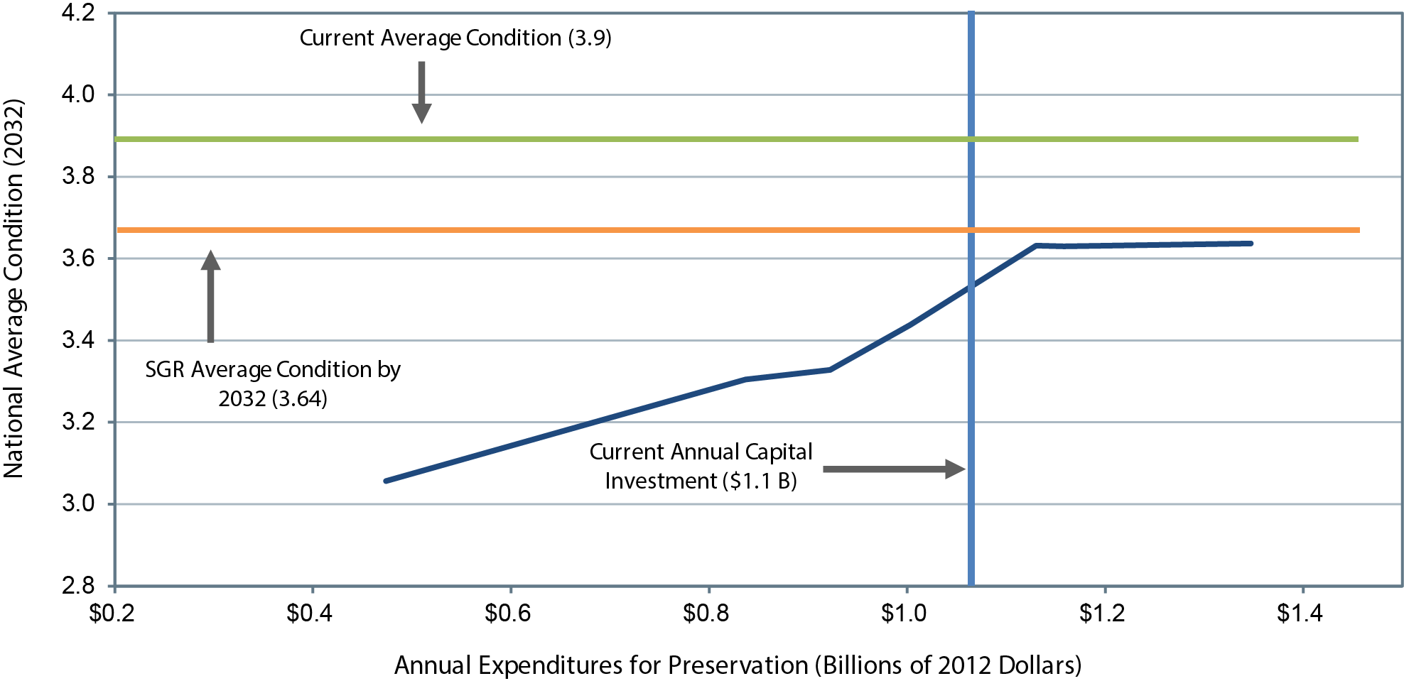
Average Annual Investment (Billions of 2012 Dollars) Total Capital Outlay	Average Annual percent Change vs. 2012	Average Transit Conditions in 2032						Funding Level Description
		Asset Categories					All Transit Assets³
		Guideway	Facilities	Systems	Stations	Vehicles	All Transit Assets³
$1.3	1.4%	4.29	3.18	3.47	4.00	3.36	3.64	SGR (unconstrained, replace at 2.50)
$1.2	0.6%	4.22	2.57	3.40	3.18	3.42	3.63	Maintain current backlog
$1.1	0.0%	4.35	2.57	3.42	3.84	3.42	3.63	2012 capital expenditures (maintain current spending)
$1.0	-1.2%	3.89	2.57	3.02	3.84	3.35	3.44	Reduce 2.5 percent
$0.9	-2.4%	3.63	2.57	3.00	3.61	3.29	3.33	Reduce 5 percent
$0.8	-3.6%	3.63	2.57	2.99	3.61	3.25	3.30	Reduce 10 percent
$0.5	-9.4%	3.63	2.57	2.99	3.61	2.81	3.06	Reduce 20 percent
¹ The conditions of individual transit assets are estimated using TERM's asset decay curves, which estimate asset conditions on a scale of 5 (excellent) through 1 (poor), as described earlier in this chapter and in Appendix C to this report. The average national condition is the weighted average of the condition of all assets nationwide, weighted by the estimated replacement cost of each asset. ² This preservation analysis is intended to consider reinvestment needs only for existing transit assets (as of 2012), not for expansion assets to be added to the existing capital stock in future years. ³ Data points depicted in the chart might not correspond exactly to data presented in the associated table due to rounding of Average Annual Investment (Billions of 2012 Dollars) amounts. Source: Transit Economic Requirements Model.

Expansion Investments

Although the urbanized and rural areas in this group represent fewer riders and a smaller existing transit asset base, these areas are also expected to have a higher projected rate of increase in transit ridership.

Exhibit 7-28 presents estimates of the level of expansion investment required to support varying levels of growth in transit demand while maintaining current performance levels (as measured by transit passenger miles per peak vehicle) for the smaller urbanized and all rural areas. Note that the 2012 level of investment for these areas ($0.5 billion) was the same as that required to support the rate of increase in transit demand as projected by the Low-Growth trend and less than the High-Growth trend rate of increase as experienced over the past several years. Such investments should yield improvements in transit performance in these urbanized areas and help promote transit-led urban development in urbanized areas subject to above average rates of population and transit growth.

Exhibit 7-28 New Ridership Supported in 2032 by Expansion Investments in Urbanized Areas with Population under 1 Million and Rural Areas¹

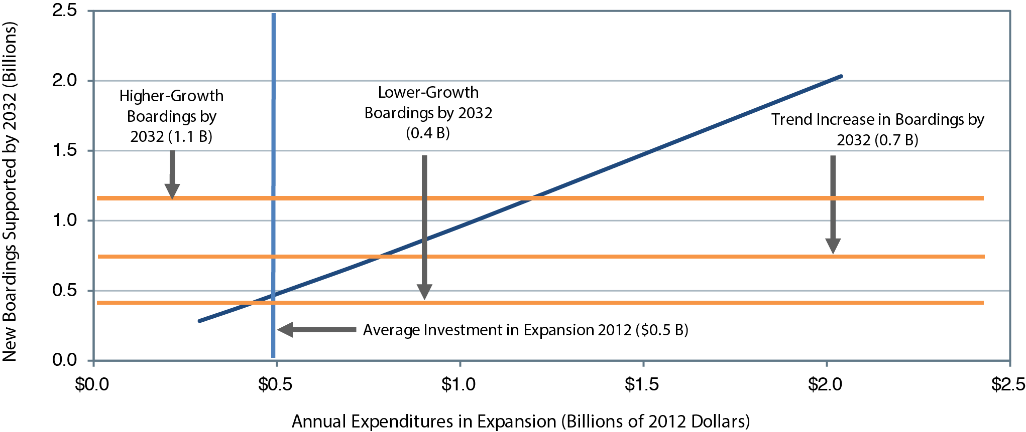
A line chart plots new boardings supported by the year 2032 over annual expenditures in expansion. The plot has an initial value of 0.3 billion new riders supported annually at an annual expenditure of $0.3 billion, and trends upward to a value of 2.0 billion new riders supported at an annual expenditure of $2.0 billion. The plot intersects with the trend increase of 0.7 billion in boardings by 2032 at an annual expenditure of $0.7 billion.<em>Source: Transit Economic Requirements Model.

Average Annual Investment (Billions of 2012 Dollars)	Average Annual percent Change vs. 2012	Total New Boardings by 2032		Funding Level Description
Average Annual Investment (Billions of 2012 Dollars)	Average Annual percent Change vs. 2012	New Riders Supported (Billions of Annual Boardings)²	Average Annual Growth in Boardings³	Funding Level Description
$2.0	12.4%	2.0	5.2%	Highest-growth scenario (+1.5%)
$1.1	7.2%	1.1	3.3%	Higher-growth scenario (+1.0%)
$0.9	5.4%	0.9	2.8%	High-growth scenario (+0.5%)
$0.7	3.4%	0.7	2.3%	15-year historic growth rate trend
$0.5	0.8%	0.5	1.9%	Low-growth scenario (-0.5%)
$0.4	-2.0%	0.4	1.5%	Lower-growth scenario (-1.0%)
$0.3	-5.9%	0.3	1.1%	Lowest-growth scenario (-1.5%)
¹ TERM assesses expansion needs at the agency-mode level subject to (1) current vehicle occupancy rates at the agency-mode level and (2) expected transit PMT growth at the UZA level (hence, all agency modes within a given UZA are subject to the same transit PMT growth rate). Note, however, that TERM does not generate expansion needs estimates for agency modes that have occupancy rates that are well below the national average for that mode. ² Data points depicted in the chart might not correspond exactly to data presented in the associated table due to rounding of Average Annual Investment (Billions of 2012 Dollars) amounts. ³ As compared with total urban ridership in 2012; only includes increases covered by investments passing TERM's benefit-cost test. Source: Transit Economic Requirements Model.

Conditions and Performance

chapter 7

Potential Highway Capital Investment Impacts

Types of Capital Spending Projected by HERS and NBIAS

Exhibit 7-1 Distribution of 2012 Capital Expenditures by Investment Type

Treatment of Traffic Growth

Alternative Levels of Future Capital Investment Analyzed

Highway Economic Requirements System

Operations Strategies

Travel Demand Elasticity

Impacts of Federal-Aid Highway Investments Modeled by HERS

Selection of Investment Levels for Analysis

Exhibit 7-2 HERS Annual Investment Levels Analyzed for Federal-Aid Highways

Investment Levels and BCRs by Funding Period

Exhibit 7-3 Minimum and Average Benefit-Cost Ratios (BCRs) for Different Possible Funding Levels on Federal-Aid Highways

Impact of Future Investment on Highway Pavement Ride Quality

Exhibit 7-4 Projected 2032 Pavement Ride Quality Indicators on Federal-Aid Highways Compared with 2012 for Different Possible Funding Levels

Impact of Future Investment on Highway Operational Performance

Exhibit 7-5 Projected Changes in 2032 Highway Travel Delay and Speed on Federal-Aid Highways Compared with Base Year for Different Possible Funding Levels

Impact of Future Investment on Highway User Costs

Exhibit 7-6 Projected 2032 Average Total User Costs on Federal-Aid Highways Compared with Base Year for Different Possible Funding Levels

Impact on Vehicle Operating Costs

Exhibit 7-7 Projected 2032 Vehicle Operating Costs on Federal-Aid Highways Compared with Base Year for Different Possible Funding Levels

Impact of Future Investment on Future VMT

Exhibit 7-8 Projected 2032 User Costs and VMT on Federal-Aid Highways Compared with Base Year for Different Possible Funding Levels

Impacts of NHS Investments Modeled by HERS

Impact of Future Investment on NHS User Costs and VMT

Exhibit 7-9 HERS Investment Levels Analyzed for the National Highway System and Projected Minimum Benefit-Cost Ratios, User Costs, and Vehicle Miles Traveled

Impact of Future Investment on NHS Travel Times and Travel Time Costs

Exhibit 7-10 Projected Changes in 2032 Highway Speed, Travel Delay, and Travel Time Costs on the National Highway System Compared with Base Year for Different Possible Funding Levels

Impact of Future Investment on NHS Pavement Ride Quality

Exhibit 7-11 Projected 2032 Pavement Ride Quality Indicators on the National Highway System Compared with 2012 for Different Possible Funding Levels

Impacts of Interstate System Investments Modeled by HERS

Impact of Future Investment on Interstate User Costs and VMT

Exhibit 7-12 HERS Investment Levels Analyzed for the Interstate System and Projected Minimum Benefit-Cost Ratios, User Costs, and Vehicle Miles Traveled

Impact of Future Investment on Interstate System Travel Times and Travel Costs

Exhibit 7-13 Projected Changes in 2032 Highway Speed, Travel Delay, and Travel Time Costs on the Interstate System Compared with Base Year for Different Possible Funding Levels

Impact of Future Investment on Interstate Pavement Ride Quality

Exhibit 7-14 Projected 2032 Pavement Ride Quality Indicators on the Interstate System Compared with 2012 for Different Possible Funding Levels

National Bridge Investment Analysis System

Performance Measures

Impacts of Systemwide Investments Modeled by NBIAS

Exhibit 7-15 Projected Impact of Alternative Investment Levels on 2032 Bridge Condition Indicators for All Bridges

Impacts of Federal-Aid Highway Investments Modeled by NBIAS

Exhibit 7-16 Projected Impact of Alternative Investment Levels on 2032 Bridge Condition Indicators for Bridges on Federal-Aid Highways

Impacts of NHS Investments Modeled by NBIAS

Exhibit 7-17 Projected Impact of Alternative Investment Levels on 2032 Bridge Condition Indicators for Bridges on the National Highway System

Impacts of Interstate Investments Modeled by NBIAS

Exhibit 7-18 Projected Impact of Alternative Investment Levels on 2032 Bridge Condition Indicators for Interstate Bridges

Potential Transit Capital Investment Impacts

Types of Capital Spending Projected by TERM

Preservation Investments

Financial Constraints, the Investment Backlog, and Future Conditions

Expansion Investments

Expansion Investments: Maintain Performance

Expansion Investments: Improve Performance

Recent Investment in Transit Preservation and Expansion

Exhibit 7-19 2012 Transit Capital Expenditures1

Impacts of Systemwide Investments Modeled by TERM

Impact of Preservation Investments on Transit Backlog and Conditions

Transit Conditions

Exhibit 7-20 Impact of Preservation Investment on 2032 Transit State of Good Repair Backlog in All Urbanized and Rural Areas

Exhibit 7-21 Impact of Preservation Investment on 2032 Transit Conditions in All Urbanized and Rural Areas1,2

Expansion Investments and Transit Ridership

Exhibit 7-22 New Ridership Supported in 2032 by Expansion Investments in All Urbanized and Rural Areas1

Impacts of Urbanized Area Investments Modeled by TERM

Urbanized Areas Over 1 Million in Population

Preservation Investments

Exhibit 7-23 Impact of Preservation Investment on 2032 Transit State of Good Repair Backlog in Urbanized Areas with Population over 1 Million

Exhibit 7-24 Impact of Level of Preservation Investment on 2032 Transit Conditions in Urbanized Areas with Population over 1 Million1,2

Expansion Investments

Other Urbanized and Rural Areas

Preservation Investments

Exhibit 7-25 New Ridership Supported in 2032 by Expansion Investments in Urbanized Areas with Population over 1 Million1

Exhibit 7-26 Impact of Preservation Investment on 2032 Transit State of Good Repair Backlog in Urbanized Areas with Population under 1 Million and Rural Areas1,2

Exhibit 7-27 Impact of Preservation Investment on 2032 Transit Conditions in Urbanized Areas with Population under 1 Million and Rural Areas1,2

Expansion Investments

Exhibit 7-28 New Ridership Supported in 2032 by Expansion Investments in Urbanized Areas with Population under 1 Million and Rural Areas1

Exhibit 7-19 2012 Transit Capital Expenditures¹

Exhibit 7-21 Impact of Preservation Investment on 2032 Transit Conditions in All Urbanized and Rural Areas^1,2

Exhibit 7-22 New Ridership Supported in 2032 by Expansion Investments in All Urbanized and Rural Areas¹

Exhibit 7-24 Impact of Level of Preservation Investment on 2032 Transit Conditions in Urbanized Areas with Population over 1 Million^1,2

Exhibit 7-25 New Ridership Supported in 2032 by Expansion Investments in Urbanized Areas with Population over 1 Million¹

Exhibit 7-26 Impact of Preservation Investment on 2032 Transit State of Good Repair Backlog in Urbanized Areas with Population under 1 Million and Rural Areas^1,2

Exhibit 7-27 Impact of Preservation Investment on 2032 Transit Conditions in Urbanized Areas with Population under 1 Million and Rural Areas^1,2

Exhibit 7-28 New Ridership Supported in 2032 by Expansion Investments in Urbanized Areas with Population under 1 Million and Rural Areas¹