

chapter 8
Selected Highway Capital Investment Scenarios
Scenarios Selected for Analysis
Scenario Derivation and Associated Spending Levels
Highway and Bridge Investment Backlog
Scenario Spending Patterns and Conditions and Performance Projections
Scenarios for the National Highway System and the Interstate System
Selected Transit Capital Investment Scenarios
Sustain 2012 Spending Scenario
State of Good Repair Benchmark
Impact on the Investment Backlog
Low-Growth and High-Growth Scenarios
Low- and High-Growth Assumptions
Low- and High-Growth Scenario Needs
Impact on Conditions and Performance
Selected Highway Capital Investment Scenarios
This section presents future investment scenarios that build on the Chapter 7 analyses of alternative levels of future investment in highways and bridges. Each scenario includes projections for system conditions and performance based on simulations with the Highway Economic Requirements System (HERS) and National Bridge Investment Analysis System (NBIAS). Each scenario scales up the total amount of simulated investment to account for capital improvements (highway and bridge investments) that are beyond the scopes of the models. Later in this chapter, transit investment scenarios are explored that, like those of this section, start with 2012 as the base year and cover the 20-year period through 2032. All scenarios are illustrative, and none is endorsed as a target level of funding.
Supplemental analyses relating to these scenarios, including comparisons with the investment levels presented for comparable scenarios in previous C&P reports, are the subject of Chapter 9. A series of sensitivity analyses that explore the implications of alternative technical assumptions for the scenario investment levels is presented in Chapter 10. The Introduction to Part II provides essential background information relating to the technical limitations of the analysis, which are discussed further in the appendices.
Scenarios Selected for Analysis
This section examines three scenarios (described in Exhibit 8-1) based on capital investment by all levels of government combined. What portion should be funded by the Federal government, State governments, local governments, or the private sector is beyond the scope of this report. Analyses were conducted first for the entire road network (titled "All Roads" in the exhibits) and then separately for Federal-aid highways, the National Highway System (NHS), and the Interstate System (these subsets of the road network are explained in Chapter 2). Each scenario pairs an assumed level of total investment in the types of improvements HERS models with an assumed level of investment in the types of improvements NBIAS models; these levels are drawn from those considered in Chapter 7. Together, the scopes of HERS and NBIAS cover spending on highway expansion and pavement improvements on Federal-aid highways (HERS) and spending on bridge rehabilitation on all highways (NBIAS). In the absence of data required for other types of highway and bridge investment (those not modeled in HERS or NBIAS), each scenario simply assumes that the percentage of highway and bridge investment spent on nonmodeled investments remains at the 2012 percentage. Percentage shares from 2012 also serve as a way to distribute the amount of nonmodeled investment among the component categories: pavement spending on non-Federal-aid highways, system expansion spending on non-Federal-aid highways, and system enhancement spending (which includes safety enhancements, operational improvements, and environmental projects) on all roads.
Exhibit 8-1 Capital Investment Scenarios for Highways and Bridges and Derivation of Components |
||||
|---|---|---|---|---|
| Scenario Component | Sustain 2012 Spending Scenario | Maintain Conditions and Performance Scenario | Improve Conditions and Performance Scenario | State of Good Repair Benchmark |
| HERS-Derived | Sustain spending on types of capital improvements modeled in HERS at 2012 levels in constant dollar terms over next 20 years. | Set spending at the lowest level at which (1) projected average IRI in 2032 matches (or is better than) the value in 2012 and (2) projected average delay per VMT in 2032 matches (or is better than) the value in 2012. | Set spending at the level sufficient to gradually fund all cost-beneficial potential projects (i.e., those with a BCR greater than or equal to 1.0) over 20 years. | Subset of Improve Conditions and Performance scenario; includes spending on system rehabilitation, excludes spending on system capacity. |
| NBIAS-Derived | Sustain spending on types of capital improvements modeled in NBIAS at 2012 levels in constant dollar terms over the next 20 years. | Set spending at the level at which the projected percentage of deck area on deficient (structurally deficient or functionally obsolete) bridges in 2032 matches that in 2012. | Set spending at the level sufficient to gradually fund all cost-beneficial potential projects over 20 years. | Includes all NBIAS-derived spending included in the Improve Conditions and Performance scenario. |
| Other (Nonmodeled) | Sustain spending on types of capital improvements not modeled in HERS or NBIAS at 2012 levels in constant dollar terms over the next 20 years. | Set spending at the level necessary so that the nonmodeled share of total highway and bridge investment will remain the same as in 2012. | Set spending at the level necessary so that the nonmodeled share of total highway and bridge investment will remain the same as in 2012. | Subset of Improve Conditions and Performance scenario; includes spending on system rehabilitation, excludes spending on system capacity and system enhancement. |
The projections for conditions and performance in each scenario are estimates of what could be achieved with a given level of investment assuming an economically driven approach to project selection (the project selection method is explained in Chapter 7). The projections do not necessarily represent what would be achieved given current decision-making practices. Consequently, comparing the relative conditions and performance outcomes across the different scenarios might be more illuminating than focusing on the specific projections for each scenario individually.

The Federal share of total capital spending on highways was 43.1 percent in 2012. Over the past 20 years, the share has ranged from a low of 37.1 percent (1998) to a high of 46.1 percent (2002). The remainder of capital spending is funded by States, local governments, and the private sector. Due to data limitations, however, separately identifying the shares for those funding sources is not possible.
As the base year of the analysis for this report is 2012 rather than 2010, the Sustain 2012 Spending scenario replaces the Sustain 2010 Spending scenario analyzed in the 2013 C&P Report. The names and definitions of the Improve Conditions and Performance scenario and the State of Good Repair benchmark are unchanged.
The Maintain Conditions and Performance scenario is similar in concept to the comparable scenario in the 2013 C&P Report, in that it attempts to maintain selected performance measures at their base-year levels through the end of the 20-year analysis period; however, the target measures have been modified. The NBIAS-derived component of the scenario targets the percentage of total bridge deck area that is on bridges classified as deficient (structurally deficient or functionally obsolete), whereas in the 2013 C&P Report, the target was the average bridge sufficiency rating. The HERS-derived component of this scenario used for the current edition is defined as the lowest investment level that is sufficient to maintain the current average IRI (International Roughness Index) and current average delay. In practice, this approach results in one of these target measures maintaining its current level and the other improving somewhat over 20 years. This approach differs from the method used in the 2013 C&P Report, which used the average of the investment level estimated to be sufficient to maintain average IRI and the investment level estimated to be sufficient to maintain average delay.
At the systemwide level, using the criteria from the 2013 C&P Report would have produced an average annual investment level of $55.4 billion, or 38.4 percent less than the $89.9 billion for the Maintain Conditions and Performance scenario shown inExhibit 8-2. This significant difference is attributable to changes to HERS and the Highway Performance Monitoring System database referenced in Chapter 7 and Appendix A. Following the integration of new pavement performance models, highway-capacity estimation formulas, new pavement distress data, new widening feasibility data, and less-aggressive forecasts of future highway demand, HERS now estimates relatively higher benefit-cost ratios for expansion projects and relatively lower benefit-cost ratios for resurfacing and reconstruction projects than was the case for the 2013 C&P Report. Thus, if projects are implemented in order of benefit-cost ratio (from high to low), HERS now finds that maintaining average delay is significantly cheaper than maintaining average pavement condition. Defining the Maintain Conditions and Performance scenario in the way it was used in the 2013 C&P Report would have resulted in average pavement condition worsening, which is inconsistent with the current emphasis on achieving a state of good repair.
Scenario Derivation and Associated Spending Levels
Future spending levels by scenario, summarized in Exhibit 8-2, are stated in constant 2012 dollars. (Chapter 9 illustrates how to convert these real-dollar values into nominal [future dollar] values that factor in inflation beyond 2012.) The modeling on which the scenarios are based (which is presented in Chapter 7) assumes that spending grows at an annual percentage rate that is constant over the 20-year analysis period, but which differs between the types of investments modeled by HERS and those modeled by NBIAS. (The average annual investment levels are determined by summing the amounts expended for each year from 2013 through 2032 under the scenario and dividing by 20.)
The application of the four illustrative scenarios to different highway systems produces the subscenarios displayed as columns in Exhibit 8-2. The goal of the subscenario is fulfilled for the particular highway system named, but does not necessarily force any subsystems to meet the scenario's goal individually. For example, the subscenario for Federal-aid highways in the Sustain 2012 Spending scenario fixes average annual spending on those highways at actual 2012 spending without likewise forcing the portions of that spending directed to the NHS or the Interstate System to match their 2012 levels. Differences between the level of investment for the subsystems and the corresponding base-year amounts arise because HERS and NBIAS rely on benefit-cost principles to allocate spending flexibly among potential improvements within their scope.
Exhibit 8-2 Summary of Average Annual Investment Levels by Scenario |
||||
|---|---|---|---|---|
| Scenario and Comparison Parameter | All Roads | Federal-Aid Highways | NHS | Interstate System |
| Sustain 2012 Spending Scenario | ||||
| Average annual investment (billions of 2012 dollars), for 2013 through 2032 | $105.2 | $79.0 | $54.6 | $20.5 |
| Maintain Conditions and Performance Scenario | ||||
| Average annual investment (billions of 2012 dollars), for 2013 through 2032 | $89.9 | $69.3 | $51.7 | $24.1 |
| percent difference relative to 2012 spending | -14.6% | -12.3% | -5.2% | 17.4% |
| Annual spending increase needed to support scenario investment level1 | -1.52% | -1.26% | -0.51% | 1.50% |
| Improve Conditions and Performance Scenario | ||||
| Average annual investment (billions of 2012 dollars), for 2013 through 2032 | $142.5 | $107.9 | $72.9 | $31.8 |
| percent difference relative to 2012 spending | 35.5% | 36.6% | 33.7% | 55.2% |
| Annual spending increase needed to support scenario investment level1 | 2.81% | 2.89% | 2.68% | 4.02% |
| State of Good Repair Benchmark | ||||
| Average annual investment (billions of 2012 dollars), for 2013 through 2032 | $85.3 | $64.9 | $42.2 | $18.4 |
1 This percentage represents the annual percent change for each year relative to 2012 that would be required to achieve the average annual funding level specified for the scenario in constant dollar terms. Additional increases in nominal dollar terms would be needed to offset the impact of future inflation. Negative values indicate that the average annual investment level associated with the scenario is lower than 2012 spending. Sources: Highway Economic Requirements System and National Bridge Investment Analysis System. | ||||
The Sustain 2012 Spending scenario, which fixes average annual investment to actual 2012 levels, results in average annual investment of $105.2 billion for all roads, of which $79.0 billion is for Federal-aid Highways, $54.6 billion is for NHS, and $20.5 billion is for the Interstate System.
The Maintain Conditions and Performance scenario uses average pavement roughness as measured by the International Roughness Index (IRI) and average delay per vehicle miles traveled (VMT) (both modeled in HERS) as the measures of overall highway conditions and performance that it seeks to maintain at 2012 levels. The scenario uses the percentage of total bridge deck area on bridges classified as deficient (structurally deficient or functionally obsolete, as modeled in NBIAS) as the measure of bridge conditions it seeks to maintain. Chapter 3 explains these metrics. Both HERS and NBIAS, used to simulate the scenarios, are designed to determine the investment program that minimizes the cost of achieving the scenario goal. Because HERS assumes that projects will be implemented in order of their benefit-cost ratios, the levels of investment that maintain each key highway measure (IRI and average delay per VMT) differ; consequently, this scenario incorporates the higher of those two levels. Because it is focused on overall conditions and performance, this scenario might sometimes entail improvement and sometimes deterioration in average conditions and performance on subsets of some networks. For example, when the scenario relates to maintaining average conditions and performance on Federal-aid highways, it could entail improvement to the Interstate System.
For the entire road network overall and specifically for Federal-aid highways and the NHS, the average amount of investment needed annually to maintain conditions and performance is less than actual 2012 spending. For all roads, the average annual investment level of $89.9 billion for the Maintain Conditions and Performance scenario is 14.6 percent lower than the actual 2012 capital spending of $105.2 billion. The goals of the scenario could be achieved even if capital spending declined by 1.52 percent per year over 20 years in constant dollar terms. Similar percentage decreases are evident in the scenarios for Federal-aid highways (12.3 percent ) and the NHS (5.2 percent ).
By design, the Improve Conditions and Performance scenario gradually increases funding over 20 years to implement all projects that have a benefit-cost ratio (BCR) greater than 1.0. For the Sustain 2012 Spending scenario, the amount of funding was sufficient to fund all projects with a BCR of 1.37 or greater (the minimum BCR for the Federal-aid highway subscenario was identical, as HERS only evaluates Federal-aid highways). For the Sustain 2012 Spending subscenarios focused on the NHS and Interstate System, the corresponding minimum BCR values were 1.29 and 1.54, respectively. For the Maintain Conditions and Performance scenario, the minimum BCR is 1.52 for all roads and Federal-aid highways, 1.33 for the NHS, and 1.26 for the Interstate System.
In contrast, the level of investment needed to maintain conditions and performance for the Interstate System is estimated to be 17.4 percent higher than the amount of investment directed to that system in 2012. The reasons for this result are twofold. First, spending on rehabilitation projects for the Interstate System has grown more slowly than for other subsets of the highway network (see Chapter 6), resulting in a relatively larger backlog of rehabilitation projects. Second, the Interstate System is aging and reconstruction needs likely will rise over time.
Targeting investment at a level projected to maintain base-year conditions and performance makes sense only if one is satisfied with that level of performance. The analyses reflected in the Improve Conditions and Performance scenario suggest that an economically driven approach to investment that funds all cost-beneficial improvements would substantially increase real spending on highways and bridges above base-year levels. The annual percentage increase in investment associated with implementing all cost-beneficial capital improvements is 2.81 percent for all roads, 2.89 percent for Federal-aid highways, 2.68 percent for the NHS, and 4.02 percent for the Interstate System. These levels of spending represent investment ceilings above which investing would not be cost-beneficial, even if available funding were unlimited. The average annual spending in this scenario exceeds the 2012 levels by 35.5 percent for all roads, 36.6 percent for Federal-aid highways, 33.7 percent for the NHS, and 55.2 percent for the Interstate System. For all roads, the average annual spending amount to implement all cost-beneficial investments fully is estimated to be $142.5 billion-or $2.9 trillion for the 20-year period-stated in constant 2012 dollars.
The State of Good Repair benchmark represents the portion of average annual spending that the Improve Conditions and Performance scenario allocates to system rehabilitation investments. Put at $85.3 billion in Exhibit 8-2 for all roads, this benchmark represents the amount of cost-beneficial investment identified for rehabilitating existing pavements and bridges. In determining the size of this benchmark, HERS and NBIAS screen out through benefit-cost analysis any assets that might have outlived their original purpose, rather than automatically reinvest in all assets in perpetuity. With national consensus lacking on exactly what constitutes a "state of good repair" for the various transportation assets, alternative benchmarks with different objectives could be equally valid from a technical perspective.
The average annual investment level for the State of Good Repair benchmark for all roads is $85.3 billion. That value is 37.3 percent higher than the $62.1 billion all levels of government spent in 2012 for all roads on system rehabilitation. The $64.9-billion State of Good Repair benchmark value for Federal-aid highways is 39.5 percent higher than the comparable 2012 spending-$46.5 billion. The $42.2-billion State of Good Repair benchmark estimate for the NHS is 33.2 percent higher than the estimated $31.6 billion spent on roads included on the NHS (following its expansion under MAP21) for system rehabilitation. The $18.4-billion State of Good Repair benchmark value for Federal-aid highways is 44.8 percent higher than comparable 2012 spending ($12.7 billion).
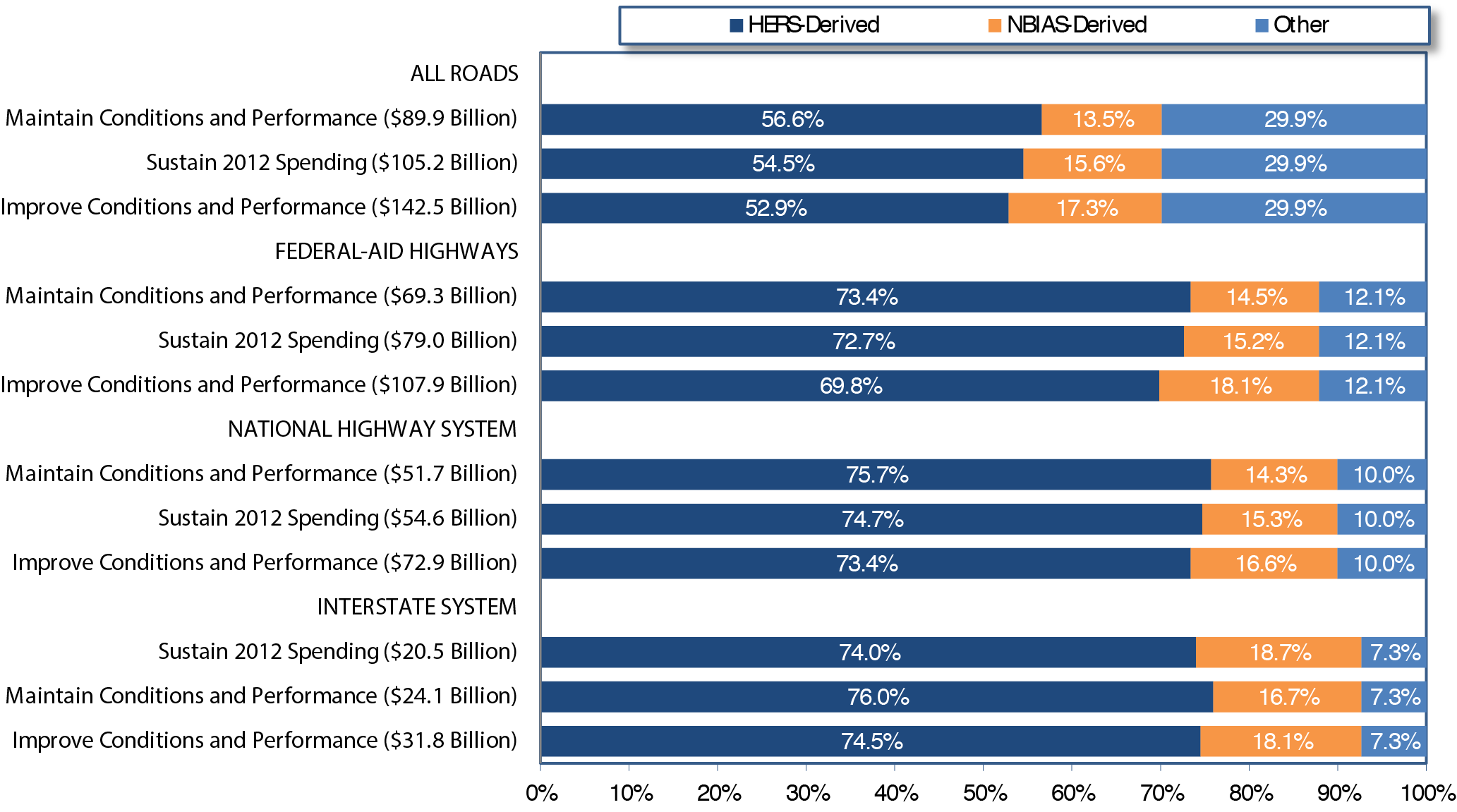
The sources of the estimates of average annual investment levels are presented in Exhibit 8-3. The HERS-derived component, which accounts for most of the total investment in each scenario, represents spending on pavement rehabilitation and capacity expansion on Federal-aid highways.
Exhibit 8-3 Source of Estimates of Highway Investment Scenarios, by Model
Sources: Highway Economic Requirements System and National Bridge Investment Analysis System.
The NBIAS-derived component represents rehabilitation spending on all bridges, including those not on Federal-aid highways. Nonmodeled spending, which accounted for 29.9 percent of total investment in 2012, is assumed to comprise the same share in all systemwide scenarios. Similarly, nonmodeled spending ("other" in Exhibit 8-3) is held constant across all scenarios at 12.1 percent for Federal-aid highways, at 10.0 percent for the NHS, and at 7.3 percent for the Interstate System.
Highway and Bridge Investment Backlog
Exhibit 8-4 presents an estimate of the 2012 backlog for the types of capital improvements modeled in HERS and NBIAS, plus an adjustment factor for nonmodeled capital improvement types. The investment backlog represents all highway and bridge improvements that could be economically justified for immediate implementation, based solely on the current conditions and operational performance of the highway system (without regard to potential future increases in VMT or potential future physical deterioration of infrastructure assets). Conceptually, this backlog represents a subset of the investment levels reflected in the Improve Conditions and Performance scenario, which addresses the existing backlog plus additional projected pavement, bridge, and capacity needs that might arise over the next 20 years.
Exhibit 8-4 Estimated Highway and Bridge Investment Backlog as of 2012 |
|||||||
|---|---|---|---|---|---|---|---|
| System Component | Billions of 2012 Dollars1 | percent of Total | |||||
| System Rehabilitation | System Expansion | System Enhancement | Total | ||||
| Highway | Bridge | Total | |||||
| Federal-aid highways-rural | $94.2 | $32.7 | $126.9 | $15.6 | $21.7 | $164.2 | 19.6% |
| Federal-aid highways-urban | $235.8 | $73.1 | $308.9 | $117.5 | $54.2 | $480.6 | 57.5% |
| Federal-aid highways-total | $330.0 | $105.8 | $435.8 | $133.1 | $75.9 | $644.8 | 77.1% |
| Non-Federal-aid highways | $89.5 | $17.3 | $106.8 | $33.9 | $50.4 | $191.2 | 22.9% |
| All Roads | $419.5 | $123.1 | $542.6 | $167.0 | $126.4 | $836.0 | 100.0% |
| Interstate System | $62.2 | $40.2 | $102.3 | $42.9 | $11.5 | $156.8 | 18.8% |
| National Highway System | $184.1 | $74.2 | $258.3 | $97.1 | $39.6 | $394.9 | 47.2% |
1 Italicized values are estimates for those system components and capital improvement types not modeled in HERS or NBIAS, such as system enhancements and pavement and expansion improvements to roads functionally classified as rural minor collector, rural local, or urban local for which Highway Performance Monitoring System data are not available to support a HERS analysis. Sources: Highway Economic Requirements System and National Bridge Investment Analysis System. | |||||||
Of the estimated $836.0-billion total backlog, approximately $156.8 billion (18.8 percent ) is for the Interstate System, $394.9 billion (47.2 percent ) is for the NHS, and $644.8 billion (77.1 percent ) is for Federal-aid highways.
Approximately 64.9 percent ($542.6 billion) of the total backlog is attributable to system rehabilitation needs, 20.0 percent ($167.0 billion) is for system expansion, and 15.1 percent ($126.4 billion) for system enhancement. The share of the total backlog attributable to system rehabilitation is roughly similar across all highway systems.
The $836.0-billion estimated backlog is heavily weighted toward urban areas; approximately 57.5 percent of this total is attributable to Federal-aid highways in urban areas. As noted in Chapter 3, average pavement ride quality on Federal-aid highways is worse in urban areas than in rural areas; urban areas also face relatively greater problems with congestion and functionally obsolete bridges than do rural areas. Very little of the backlog spending (just 1.9 percent ) is targeted toward system expansion on rural Federal-aid highways.
Scenario Spending Patterns and Conditions and Performance Projections
Systemwide Scenarios
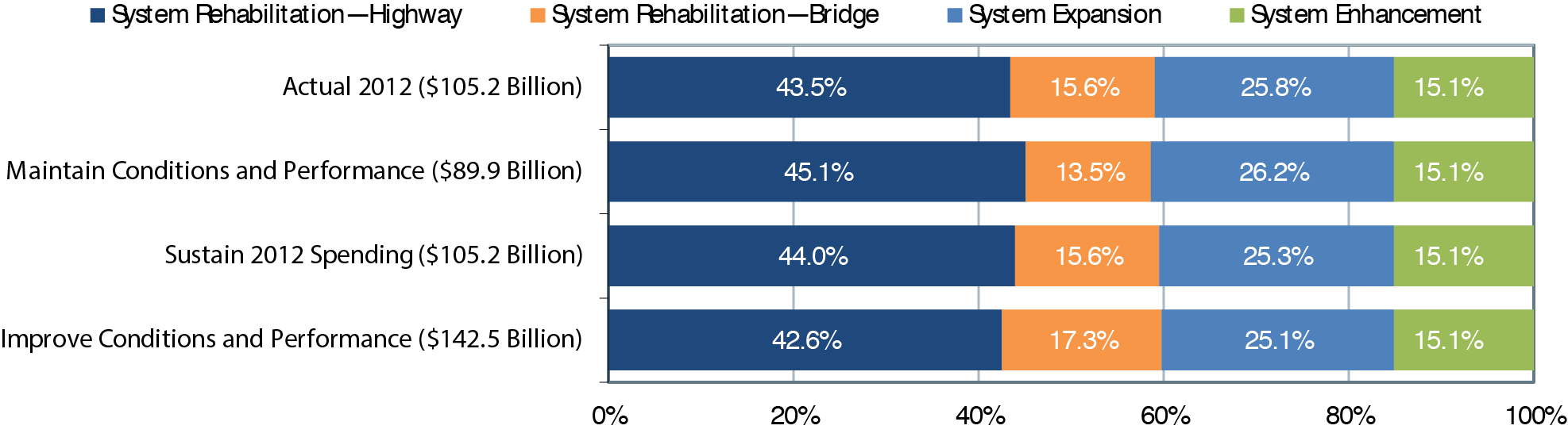
The systemwide distribution of spending among improvement types for each scenario is shown in Exhibit 8-5. In the Improve Conditions and Performance scenario, annual spending on highway and bridge rehabilitation averages $85.3 billion, considerably more than the $62.1 billion of such spending in 2012 identified in Chapter 6. This result suggests that achieving a state of good repair on the Nation's highways would require either a significant increase in overall highway and bridge investment or a significant redirection of investment from other types of improvements toward system rehabilitation.
Exhibit 8-5 Systemwide Highway Capital Investment Scenarios for 2013 Through 2032: Distribution by Capital Improvement Type Compared with Actual 2012 Spending
| Capital Improvement Type | Actual 2012 Spending Distribution | Sustain 2012 Spending Scenario | Maintain Conditions & Performance Scenario | Improve Conditions & Performance Scenario |
|---|---|---|---|---|
| Average Annual Distribution by Capital Improvement Type (Billions of 2012 Dollars) | ||||
| System rehabilitation-highway | $45.7 | $46.3 | $40.6 | $60.7 |
| System rehabilitation-bridge | $16.4 | $16.4 | $12.2 | $24.6 |
| System rehabilitation-total | $62.1 | $62.7 | $52.7 | $85.3 |
| System expansion | $27.2 | $26.6 | $23.6 | $35.7 |
| System enhancement | $15.9 | $15.9 | $13.6 | $21.5 |
| Total, All Improvement Types | $105.2 | $105.2 | $89.9 | $142.5 |
|
Sources: Highway Economic Requirements System and National Bridge Investment Analysis System. | ||||
Exhibit 8-5 compares the distributions from each scenario for investment spending by improvement type with the actual distribution of capital spending in 2012. At first glance, the proportional splits between improvement types roughly match the current 2012 spending by improvement type. Of importance to note, however, is that each percentage point change represents an approximate $1-billion shift in spending. Comparing the Sustain 2012 Spending scenario to the Actual 2012 Spending scenario, HERS modeling results support less spending on system expansion and more spending on highway rehabilitation than actually occur. At the higher levels of spending implied by the Improve Conditions and Performance scenario, the modeling results suggest spending relatively more on bridge system rehabilitation and relatively less on highway system rehabilitation and system expansion.
Exhibit 8-6 presents conditions and performance indicators for systemwide scenarios. (This information also can be found in various tables in Chapter 7). Because HERS considers only Federal-aid highways, the indicators for the Federal-aid highway scenarios are presented in place of indicators for all roads in Exhibit 8-6. These results are discussed more fully in the Federal-aid highway section below. In contrast, NBIAS considers bridges on all roads and provides several indicators to describe conditions and performance.
Exhibit 8-6 Systemwide Highway Capital Investment Scenarios for 2013 Through 2032: Projected Impacts on Selected Highway Performance Measures
| Highway Performance Measure | Actual 2012 Values | Sustain 2012 Spending Scenario | Maintain Conditions & Performance Scenario | Improve Conditions & Performance Scenario |
|---|---|---|---|---|
| Projected 2032 Values for Selected NBIAS Indicators (for Which Lower Numbers are Better) | ||||
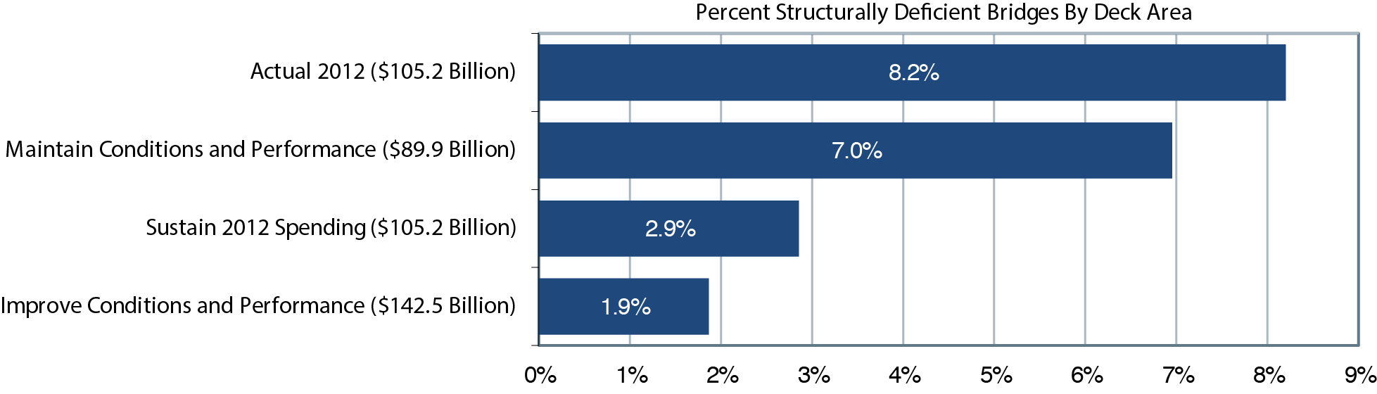
| percent structurally deficient bridges by deck area | 8.2% | 2.9% | 7.0% | 1.9% |
| Total percent deficient bridges by deck area | 26.7% | 22.9% | 26.7% | 21.2% |
| Economic bridge investment backlog (billions of 2012 dollars) | $123.1 | $20.3 | $67.6 | $0.0 |
| Projected 2032 Values for Selected HERS Indicators (for Which Higher Numbers are Better) | ||||
| percent of VMT on roads with good ride quality1 | 44.9% | 50.8% | 46.0% | 60.9% |
| percent of VMT on roads with acceptable ride quality1 | 83.3% | 87.7% | 85.9% | 91.5% |
| Projected Changes by 2032 Relative to 2012 for Selected HERS Indicators (for Which Negative Numbers are Better) | ||||
| percent change in average IRI (VMT-weighted)1 | 0.0% | -4.5% | 0.0% | -14.0% |
| percent change in average delay per VMT1 | 0.0% | -13.4% | -12.2% | -16.5% |
1 The HERS indicators shown apply only to Federal-aid highways as HPMS sample data are not available for rural minor collectors, rural local, or urban local roads. Sources: Highway Economic Requirements System and National Bridge Investment Analysis System. | ||||
Under the Sustain 2012 Spending scenario, the economic bridge investment backlog would drop from $123.1 billion in 2012 to $20.3 billion in 2032 and total percentage of bridges by deck area that are deficient would drop from 26.7 percent to 22.9 percent . The percentage of VMT on roads with good ride quality would rise from 44.9 percent to 50.8 percent and the average IRI would improve by 4.5 percent , while the average delay per VMT would fall by 13.4 percent .
The cells shaded blue in Exhibit 8-6 (and similar exhibits that follow) are the values that define the scenarios. For the Maintain Conditions and Performance scenario, the cell showing that 26.7 percent of bridges (as measured by deck area) in 2032 would be deficient is shaded blue as it matches the actual value in 2012 (the goal of that scenario is to set funding to a level sufficient to maintain bridge conditions at their 2012 level). The cell showing that the average change in VMT-weighted IRI is 0.0 percent also is shaded blue, showing that this metric is unchanged relative to the actual 2012 value. Under the Maintain Conditions and Performance scenario, the economic bridge investment backlog would be $67.6 billion in 2032.
For the Improve Conditions and Performance scenario, the cell showing $0.0 in economic bridge investment backlog is shaded blue because the target of that scenario is to set spending at a level that would fund all cost-beneficial projects (thus eliminating the backlog). Under the Improve Conditions and Performance scenario, the percentage of bridges (measured by deck area) that are structurally deficient is projected to drop from 8.2 percent in 2012 to 1.9 percent in 2032. The total percentage of deficient bridges (including structurally deficient or functionally obsolete bridges) by deck area would drop from 26.7 percent in 2012 to 21.2 percent under the Improve Conditions and Performance scenario. (Of note is that this statistic understates the likely reduction in functionally obsolete bridges under this scenario, as it only captures improvements modeled in NBIAS and thus does not reflect the potential impact that system expansion investments modeled in HERS might have on addressing functionally obsolete bridges by replacing them with wider bridges). The Improve Conditions and Performance scenario also would eliminate the total economic bridge investment backlog, which totaled $123.1 in 2012.
Federal-Aid Highway Scenarios
For the scenarios that focus on Federal-aid highways, the average annual investment totals and the breakdown of those funds by type of investment are shown in Exhibit 8-7. The Maintain Conditions and Performance scenario involves a $9.7-billion reduction in spending on Federal-aid highways and the resulting lower level of spending would be allocated to different types of improvements in roughly the same proportion as actual 2012 spending. The Improve Conditions and Performance scenario involves an increase of $28.9 billion in spending per year, on average. At this higher level of spending, relatively more spending is directed toward rehabilitation and relatively less toward system expansion. System rehabilitation received 58.9 percent of funds in 2012 but would receive 60.1 percent under the Improve Conditions and Performance scenario.
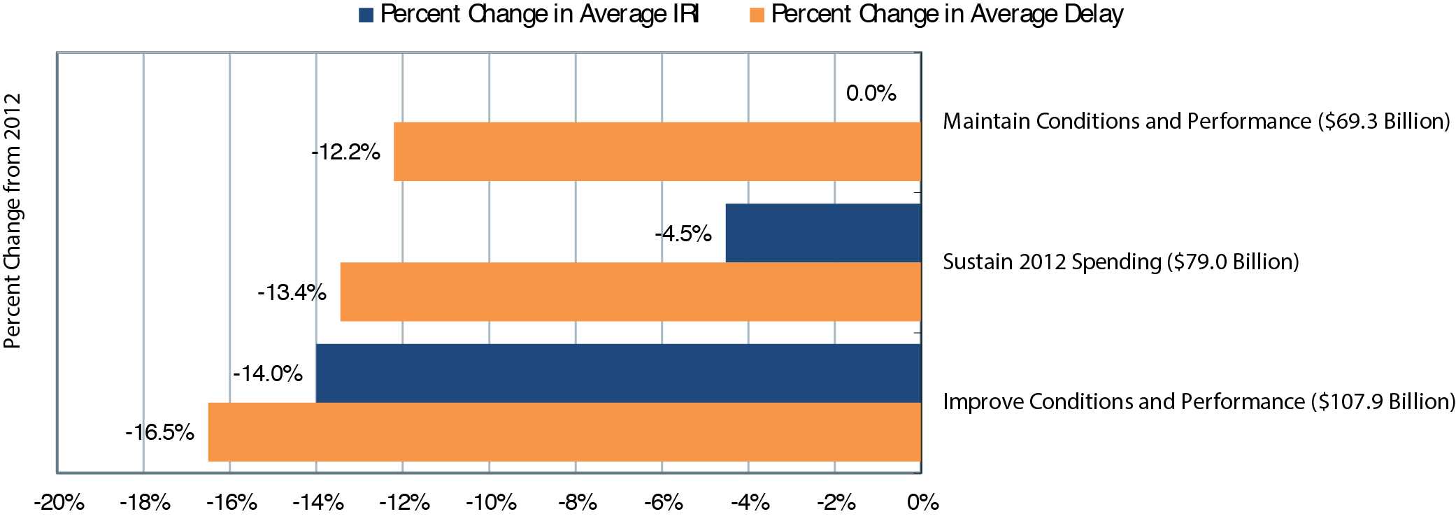
Exhibit 8-8 presents conditions and performance indicators for the Federal-aid highways scenarios. Regarding performance indicators for roads, in 2012, the percentage of all VMT on roads in the Federal-aid highway system with good ride quality was 44.9 percent . That indicator would reach 60.9 percent under the Improve Conditions and Performance scenario. The Improve Conditions and Performance scenario raises the percentage of VMT on roads with acceptable ride quality to 91.5 percent from the 2012 value of 83.3 percent . The average VMT-weighted IRI (for which lower numbers are better) would improve by 14.0 percent from its 2012 value under the Improve Conditions and Improvement scenario. The average delay per VMT would improve by 16.5 percent from its 2012 value under the Improve Conditions and Performance scenario, by 12.2 percent under the Maintain Conditions and Performance and by 13.4 percent in the Sustain 2012 Spending scenario. The reason average delay per VMT improves while spending remains constant or decreases is that capacity expansion projects tend to yield relatively high benefit-cost ratios, thus HERS opts to fund those projects, even when only limited funding is available. This level of forecast improvement in average delay per VMT is a departure from the findings of the 2013 C&P Report. This difference is due to changes in the modeling approach, discussed in Chapter 7, and because the forecast growth in VMT for this analysis is significantly lower than the growth rates used in the previous analysis. The 2013 C&P Report provides results for assumed annual VMT growth rates of 1.85 percent and 1.36 percent , while this current analysis assumes a VMT growth rate of 1.04 percent .
Exhibit 8-7 Federal-Aid Highway Capital Investment Scenarios for 2013 Through 2032: Distribution by Capital Improvement Type Compared with Actual 2012 Spending |
||||
|---|---|---|---|---|
| Capital Improvement Type | Actual 2012 Spending Distribution | Sustain 2012 Spending Scenario | Maintain Conditions & Performance Scenario | Improve Conditions & Performance Scenario |
| Average Annual Distribution by Capital Improvement Type (Billions of 2012 Dollars) | ||||
| System rehabilitation-highway | $34.5 | $35.0 | $30.9 | $45.4 |
| System rehabilitation-bridge | $12.0 | $12.0 | $10.0 | $19.5 |
| System rehabilitation-total | $46.5 | $47.0 | $41.0 | $64.9 |
| System expansion | $22.9 | $22.4 | $19.9 | $30.0 |
| System enhancement | $9.6 | $9.6 | $8.4 | $13.1 |
| Total, all improvement types | $79.0 | $79.0 | $69.3 | $107.9 |
| Percent Distribution by Capital Improvement Type | ||||
| System rehabilitation | 58.9% | 59.6% | 59.1% | 60.1% |
| System expansion | 29.0% | 28.3% | 28.8% | 27.8% |
| System enhancement | 12.1% | 12.1% | 12.1% | 12.1% |
|
Sources: Highway Economic Requirements System and National Bridge Investment Analysis System. | ||||
Exhibit 8-8 Federal-Aid Highway Capital Investment Scenarios for 2013 Through 2032: Projected Impacts on Selected Highway Performance Measures
| Highway Performance Measure | Actual 2012 Values | Sustain 2012 Spending Scenario | Maintain Conditions & Performance Scenario | Improve Conditions & Performance Scenario |
|---|---|---|---|---|
| Projected 2032 Values for Selected NBIAS Indicators (for Which Lower Numbers are Better) | ||||
| percent structurally deficient by deck area | 7.5% | 3.3% | 6.3% | 1.2% |
| Total percent deficient bridges by deck area | 26.6% | 24.0% | 26.6% | 21.1% |
| Economic bridge investment backlog (billions of 2012 dollars) | $105.8 | $28.1 | $55.9 | $0.0 |
| Projected 2032 Values for Selected HERS Indicators (for Which Higher Numbers are Better) | ||||
| percent of VMT on roads with good ride quality | 44.9% | 50.8% | 46.0% | 60.9% |
| percent of VMT on roads with acceptable ride quality | 83.3% | 87.7% | 85.9% | 91.5% |
| Projected Changes by 2032 Relative to 2012 for Selected HERS Indicators (for Which Negative Numbers are Better) | ||||
| percent change in average IRI (VMT-weighted) | 0.0% | -4.5% | 0.0% | -14.0% |
| percent change in average delay per VMT | 0.0% | -13.4% | -12.2% | -16.5% |
|
Sources: Highway Economic Requirements System and National Bridge Investment Analysis System. | ||||
Under the Improve Conditions and Performance scenario, the percentage of bridges in the Federal-aid highway network (measured by deck area) that are structurally deficient is projected to drop from 7.5 percent in 2012 to 1.2 percent in 2032. The total percentage classified as deficient decreases from 26.6 percent in 2012 to 21.1 percent under the Improve Conditions and Performance scenario. The Improve Conditions and Performance scenario also eliminates the total economic bridge investment backlog, which was $105.8 billion in 2012. Under the Sustain 2012 Spending scenario, the bridge backlog drops to $28.1 billion, while the Maintain Conditions and Performance scenario results in a $55.9-billion backlog in 2032.
Spending by Improvement Type and Highway Functional Class
Exhibit 8-9 presents the distribution by improvement type and highway functional class for the Improve Conditions and Performance scenario compared to actual 2012 spending for Federal-aid highways. Moving to a finer level of detail in the analysis tends to reduce the reliability of simulation results from HERS and NBIAS, so the results presented in this exhibit should be viewed with caution. Nevertheless, the patterns strongly suggest certain directions in which spending patterns would need to change for scenario goals to be achieved. The scenarios can feature shifts in spending across highway functional classes and in highway spending between rehabilitation and expansion because the modeling frameworks determine allocations through benefit-cost optimization.
The Improve Conditions and Performance scenario shows that using a benefit-cost framework for project selection would dramatically shift spending away from rural roads and toward urban roads. Spending on rural roads would decrease by 1.2 percent from actual 2012 spending to $27.7 billion, while spending on urban roads would increase 57.5 percent to $80.2 billion.
The reduced spending on rural roads derives entirely from decreases in system expansion spending, which is reduced by 64.0 percent compared to actual 2012 spending. This indicates that HERS finds that sustaining spending in rural expansion at current levels over 20 years would not be cost-beneficial. In contrast, the Improve Conditions and Performance scenario suggests that a 75.5-percent increase in funding for system expansion of urban roads would be cost-beneficial.
Exhibit 8-9 Improve Conditions and Performance Scenario for Federal-Aid Highways: Distribution of Average Annual Investment for 2013 Through 2032 Compared with Actual 2012 Spending by Functional Class and Improvement Type |
|||||||
|---|---|---|---|---|---|---|---|
| Average Annual National Investment on Federal-Aid Highways (Billions of 2012 Dollars) | |||||||
| Functional Class | System Rehabilitation | System Expansion | System Enhancement | Total | |||
| Highway | Bridge | Total | |||||
| Rural Arterials and Major Collectors | |||||||
| Interstate | $4.7 | $1.5 | $6.2 | $0.7 | $0.7 | $7.7 | |
| Other principal arterial | $5.0 | $1.0 | $6.0 | $0.8 | $1.1 | $8.0 | |
| Minor arterial | $3.1 | $0.9 | $4.0 | $0.5 | $0.8 | $5.3 | |
| Major collector | $3.6 | $1.6 | $5.2 | $0.6 | $1.0 | $6.8 | |
| Subtotal | $16.4 | $5.0 | $21.4 | $2.6 | $3.7 | $27.7 | |
| Urban Arterials and Collectors | |||||||
| Interstate | $7.4 | $4.7 | $12.2 | $9.9 | $1.3 | $23.4 | |
| Other freeway and expressway | $3.9 | $1.8 | $5.7 | $7.3 | $1.1 | $14.1 | |
| Other principal arterial | $8.2 | $3.5 | $11.7 | $4.3 | $2.9 | $18.9 | |
| Minor arterial | $6.4 | $3.2 | $9.6 | $4.0 | $2.4 | $15.9 | |
| Collector | $3.1 | $1.3 | $4.4 | $1.8 | $1.7 | $7.9 | |
| Subtotal | $29.0 | $14.5 | $43.5 | $27.3 | $9.3 | $80.2 | |
| Total, Federal-aid highways1 | $45.4 | $19.5 | $64.9 | $30.0 | $13.1 | $107.9 | |
| percent Above Actual 2012 Capital Spending on Federal-Aid Highways by All Levels of Government Combined | |||||||
| Functional Class | System Rehabilitation | System Expansion | System Enhancement | Total | |||
| Highway | Bridge | Total | |||||
| Rural Arterials and Major Collectors | |||||||
| Interstate | 28.8% | 241.9% | 51.3% | -62.4% | 36.6% | 16.8% | |
| Other principal arterial | -4.9% | 42.4% | 0.7% | -72.4% | 36.6% | -19.2% | |
| Minor arterial | 14.1% | 3.8% | 11.6% | -65.7% | 36.6% | -5.8% | |
| Major collector | 6.4% | 58.4% | 18.3% | -35.4% | 36.6% | 12.8% | |
| Subtotal | 9.3% | 65.4% | 18.7% | -64.0% | 36.6% | -1.2% | |
| Urban Arterials and Collectors | |||||||
| Interstate | 42.1% | 39.7% | 41.1% | 129.7% | 36.6% | 68.4% | |
| Other freeway and expressway | 83.9% | 159.3% | 103.0% | 180.1% | 36.6% | 127.0% | |
| Other principal arterial | 39.7% | 28.0% | 36.0% | -16.2% | 36.6% | 19.3% | |
| Minor arterial | 71.0% | 122.4% | 85.3% | 73.0% | 36.6% | 73.1% | |
| Collector | 23.6% | 62.7% | 32.7% | 46.8% | 36.6% | 36.6% | |
| Subtotal | 49.0% | 60.7% | 52.7% | 75.5% | 36.6% | 57.5% | |
| Total, Federal-aid highways1 | 31.8% | 61.9% | 39.5% | 30.7% | 36.6% | 36.6% | |
1 The term "Federal-aid highways" refers to those portions of the road network that are generally eligible for Federal funding. Roads functionally classified as rural minor collectors, rural local, and urban local are excluded, although some types of Federal program funds can be used on such facilities. Sources: Highway Economic Requirements System and National Bridge Investment Analysis System. | |||||||
Spending on system rehabilitation for rural roads increases 18.7 percent in the Improve Conditions and Performance scenario compared to actual 2012 spending, but that increase is significantly lower than the 52.7-percent increase in spending for system rehabilitation needed for urban roads. Bridges on both urban and rural roads require substantial system rehabilitation spending, however, to achieve the goals of the scenario. The Improve Conditions and Performance scenario calls for 65.4-percent and 60.7-percent increases in system rehabilitation spending over actual 2012 spending for rural and urban bridges respectively.
The Improve Conditions and Performance scenario suggests that the largest funding gaps (in percentage terms) are for bridge rehabilitation on the rural portion of the Interstate System (241.9 percent ), system expansion for urban freeways and expressways (180.1 percent ), bridge rehabilitation on urban freeways and expressways (159.3 percent ), and expansion of the urban portion of the Interstate System (129.7 percent ).
Scenarios for the National Highway System and the Interstate System
Parallel to the analysis for the Federal-aid highways, Exhibit 8-10 presents the scenarios for the NHS, and Exhibit 8-11 presents the scenarios for the Interstate System. The results from these scenarios are derived in the same way, and the only spending component that is not modeled is system enhancements. System enhancements in 2012 accounted for slightly smaller shares of spending on the NHS and Interstate System than on all Federal-aid highways. Comparison of these scenarios with the Federal-aid highway scenarios in Exhibit 8-7 reveals several patterns of interest:
- For both the NHS and the Interstate System, the Sustain 2012 Spending scenario suggests that some of the current spending should be shifted from system rehabilitation to system expansion. The suggested shift from rehabilitation to expansion is even more pronounced for the Maintain Conditions and Performance scenarios.
- The Improve Conditions and Performance scenario suggests that, with increased funding for the Interstate System, proportionally more funding should be directed at system expansion than at lower levels of funding.
- The Improve Conditions and Performance scenario suggests that the Interstate System is most in need of system expansion capital spending compared to the NHS or Federal-aid highways. The percentage of funding for system expansion is 27.8 percent for Federal-aid highways, 32.2 percent for the NHS, and 34.7 percent for the Interstate System.
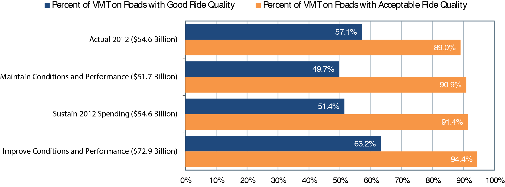
- The Improve Conditions and Performance scenario results in more substantial road improvements (for all measures except pavement roughness) for the NHS and Interstate System than for Federal-aid highways as a whole. The average delay per VMT is reduced by 49.0 percent over 2012 conditions for the Interstate System, by 27.2 percent for the NHS, and by 16.5 percent for Federal-aid highways under the Improve Conditions and Performance scenario. The percentage of VMT on roads with acceptable ride quality is 98.7 percent for the Interstate System, 94.4 percent for the NHS, and 91.5 percent for Federal-aid highways under the Improve Conditions and Performance scenario.
- The Improve Conditions and Performance scenario results in more substantial pavement roughness for Federal-aid highways as a whole than for the Interstate System and the NHS. The percentage change in VMT-weighted average IRI is -14.0 percent for Federal-aid highways, -12.0 percent for NHS, and -9.3 percent for the Interstate System.
- In 2012, 7.1 percent of bridges (measured by deck area) on the Interstate System and the NHS were structurally deficient. The Improve Conditions and Performance scenario reduces that percentage by 6.1 percentage points to 1.0 percent for both the Interstate System and the NHS.
Exhibit 8-10 National Highway System Capital Investment Scenarios for 2013 Through 2032: Distribution by Capital Improvement Type and Projected Impacts on Selected Highway Performance Measures
| Capital Improvement Type | Actual 2012 Values | Sustain 2012 Spending Scenario | Maintain Conditions & Performance Scenario | Improve Conditions & Performance Scenario |
|---|---|---|---|---|
| Distribution by Capital Improvement Type, Average Annual (Billions of Base Year Dollars) | ||||
| System rehabilitation-highway | $23.3 | $23.0 | $22.1 | $30.1 |
| System rehabilitation-bridge | $8.3 | $8.3 | $7.4 | $12.1 |
| System rehabilitation-total | $31.6 | $31.3 | $29.4 | $42.2 |
| System expansion | $17.4 | $17.8 | $17.1 | $23.5 |
| System enhancement | $5.5 | $5.5 | $5.2 | $7.3 |
| Total, all improvement types | $54.6 | $54.6 | $51.7 | $72.9 |
| Percent Distribution by Capital Improvement Type | ||||
| System rehabilitation | 58.0% | 57.4% | 56.9% | 57.8% |
| System expansion | 32.0% | 32.6% | 33.1% | 32.2% |
| System enhancement | 10.0% | 10.0% | 10.0% | 10.0% |
| Projected 2032 Values for Selected NBIAS Indicators (for Which Lower Numbers Are Better) | ||||
| percent structurally deficient by deck area | 7.1% | 3.1% | 4.9% | 1.0% |
| Total percent deficient bridges by deck area | 26.9% | 25.4% | 26.9% | 23.1% |
| Economic bridge investment backlog (billions of 2012 dollars) | $74.2 | $19.1 | $32.7 | $0.0 |
| Projected 2032 Values for Selected HERS Indicators (for Which Higher Numbers Are Better) | ||||
| percent of VMT on roads with good ride quality | 57.1% | 51.4% | 49.7% | 63.2% |
| percent of VMT on roads with acceptable ride quality | 89.0% | 91.4% | 90.9% | 94.4% |
| Projected Changes by 2032 Relative to 2012 for Selected HERS Indicators (for Which Negative Numbers Are Better) | ||||
| percent change in average IRI (VMT-weighted) | 0.0% | -1.6% | 0.0% | -12.0% |
| percent change in average delay per VMT | 0.0% | -22.9% | -22.2% | -27.2% |
|
Sources: Highway Economic Requirements System and National Bridge Investment Analysis System. | ||||
Exhibit 8-11 Interstate System Capital Investment Scenarios for 2013 Through 2032: Distribution by Capital Improvement Type and Projected Impacts on Selected Highway Performance Measures
| Capital Improvement Type | Actual 2012 Values | Sustain 2012 Spending Scenario | Maintain Conditions & Performance Scenario | Improve Conditions & Performance Scenario |
|---|---|---|---|---|
| Distribution by Capital Improvement Type, Average Annual (Billions of Base Year Dollars) | ||||
| System rehabilitation-highway | $8.9 | $8.3 | $10.1 | $12.7 |
| System rehabilitation-bridge | $3.8 | $3.8 | $4.0 | $5.8 |
| System rehabilitation-total | $12.7 | $12.2 | $14.1 | $18.4 |
| System expansion | $6.3 | $6.8 | $8.2 | $11.0 |
| System enhancement | $1.5 | $1.5 | $1.8 | $2.3 |
| Total, all improvement types | $20.5 | $20.5 | $24.1 | $31.8 |
| percent Distribution by Capital Improvement Type | ||||
| System rehabilitation | 62.1% | 59.4% | 58.6% | 58.0% |
| System expansion | 30.5% | 33.3% | 34.1% | 34.7% |
| System enhancement | 7.3% | 7.3% | 7.3% | 7.3% |
| Projected 2032 Values for Selected NBIAS Indicators (for Which Lower Numbers Are Better) | ||||
| percent structurally deficient by deck area | 7.1% | 6.6% | 5.6% | 1.0% |
| Total percent deficient bridges by deck area | 28.5% | 29.2% | 28.5% | 24.7% |
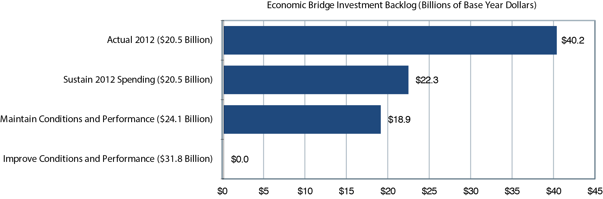
| Economic bridge investment backlog (billions of 2012 dollars) | $40.2 | $22.3 | $18.9 | $0.0 |
| Projected 2032 Values for Selected HERS Indicators (for Which Higher Numbers Are Better) | ||||
| percent of VMT on roads with good ride quality | 66.8% | 43.7% | 52.5% | 64.7% |
| percent of VMT on roads with acceptable ride quality | 95.2% | 95.1% | 97.1% | 98.7% |
| Projected Changes by 2032 Relative to 2012 for Selected HERS Indicators (for Which Negative Numbers Are Better) | ||||
| percent change in average IRI (VMT-weighted) | 0.0% | 7.9% | 0.0% | -9.3% |
| percent change in average delay per VMT | 0.0% | -31.6% | -37.9% | -49.0% |
|
Sources: Highway Economic Requirements System and National Bridge Investment Analysis System. | ||||
Selected Transit Capital Investment Scenarios
Chapter 7 considered the impacts of varying levels of capital investment on transit conditions and performance. This chapter provides in-depth analysis of four specific investment scenarios, as outlined below in Exhibit 8-12. The Sustain 2012 Spending scenario assesses the impact of sustaining current expenditure levels on asset conditions and system performance over the next 20 years. Given that current expenditure rates are generally less than are required to maintain current condition and performance levels, this scenario reflects the magnitude of the expected declines in condition and performance should current capital investment rates be maintained. The State of Good Repair (SGR) Benchmark considers the level of investment required to eliminate the existing capital investment backlog and the condition and performance impacts of doing so. In contrast to the other scenarios considered here, the SGR Benchmark considers only the preservation needs of existing transit assets (it does not consider expansion requirements). Moreover, the SGR Benchmark does not require investments to pass the Transit Economic Requirements Model's (TERM's) benefit-cost test. Hence, it brings all assets to an SGR regardless of TERM's assessment of whether reinvestment is warranted. Finally, the Low-Growth and High-Growth scenarios both assess the required levels of reinvestment to (1) preserve existing transit assets at a condition rating of 2.5 or higher and (2) expand transit service capacity to support differing levels of ridership growth while passing TERM's benefit-cost test.
Exhibit 8-12 Capital Investment Scenarios for Transit |
||||
|---|---|---|---|---|
| SGR Benchmark | Sustain 2012 Spending Scenario | Low-Growth Scenario | High-Growth Scenario | |
| Description | Level of investment to attain and maintain SGR over next 20 years (no assessment of expansion needs) | Sustain preservation and expansion spending at current levels over next 20 years | Preserve existing assets and expand asset base to support historical rate of ridership growth less 0.5% (1.3% between 1997 and 2012) | Preserve existing assets and expand asset base to support historical rate of ridership growth plus 0.5% (2.2% between 1997 and 2012) |
| Objective | Requirements to attain SGR (as defined by assets in condition 2.5 or better) | Assess impact of constrained funding on condition, SGR backlog, and ridership capacity | Assess unconstrained preservation and capacity expansion needs assuming low ridership growth | Assess unconstrained preservation and capacity expansion needs assuming high ridership growth |
| Apply Benefit- Cost Test? | No | Yes1 | Yes | Yes |
| Preservation? | Yes2 | Yes2 | Yes2 | Yes2 |
| Expansion? | No | Yes | Yes | Yes |
1 To prioritize investments under constrained funding. 2 Replace at condition 2.5. | ||||
TERM's estimates for capital expansion needs in the Low- and High-Growth scenarios are driven by the projected growth in passenger miles traveled (PMT). For this C&P report, Federal Transit Administration (FTA) has applied a new methodology for estimating growth in PMT that is considered more accurate and provides greater consistency between the Low- and High-Growth scenarios.
In prior years, PMT projections obtained from metropolitan planning organizations (MPOs) drove the Low-Growth scenario. Specially, PMT growth projections at the urbanized area (UZA) level were obtained from MPOs representing the Nation's 30 largest UZAs along with a sample of projections for MPOs representing smaller UZAs (population less than 1 million). These projections then were used to estimate transit capital expansion needs for the Low-Growth scenario. UZA growth rates for smaller UZAs not included in the sample were based on an average for UZAs of comparable size and region of the country. In contrast, the High-Growth scenario was driven by the historical (compound average annual) trend in rate of growth, also at the UZA level, based on data from the National Transit Database (NTD) for the most recent 15-year period.
For this C&P report, the Low- and High-Growth scenarios use a common, consistent approach that better reflects differences in PMT growth by mode. Specifically, these scenarios are now based on the trend rate of growth in PMT, calculated as the compound average annual PMT growth by FTA region, UZA stratum, and mode over the most recent 15-year period. For example, all bus operators located in the same FTA region in UZAs of the same population stratum are assigned the same growth rate. Use of the 10 FTA regions captures regional differences in PMT growth, while use of population strata (greater than 1 million; 1 million to 500,000; 500,000 to 250,000; and less than 250,000) captures differences in urban area size. Perhaps more importantly, the revised approach now recognizes differences in PMT growth trends by transit mode. Over the past decade, the rate of PMT growth has differed markedly across transit modes: highest for heavy rail, vanpool, and demand response and low to flat for motor bus. These differences are now accounted for in the expansion need projections for the Low- and High-Growth scenarios.
Exhibit 8-13 summarizes the analysis results for each scenario. Note that each scenario presented in Exhibit 8-13 imposes the same asset condition replacement threshold (i.e., assets are replaced at condition rating 2.5 when budget is sufficient) when assessing transit reinvestment needs. Hence, the differences in the total preservation expenditure amounts across each scenario primarily reflect the impact of either (1) an imposed budget constraint (Sustain 2012 Spending scenario) or (2) application of TERM's benefit-cost test (the SGR Benchmark does not apply the benefit-cost test). A brief review of Exhibit 8-13 reveals the following:
- SGR Benchmark: The level of expenditures required to attain and maintain an SGR over the upcoming 20 years, which would cover preservation needs but excludes expansion investments, is 8.6 percent higher than that currently expended on asset preservation and expansion combined.
- Sustain 2012 Spending Scenario: Total spending under this scenario is well below that of the other scenarios, indicating that sustaining recent spending levels is insufficient to attain the investment objectives of the SGR Benchmark, the Low-Growth scenario, or the High-Growth scenario. This result suggests future increases in the size of the SGR backlog and a likely increase in the number of transit riders per peak vehicle-including an increased incidence of crowding-in the absence of increased expenditures.
- Low and High-Growth Scenarios: The level of investment to address expected preservation and expansion needs is estimated to be roughly 46 to 69 percent higher than currently expended by the Nation's transit operators. Preservation and expansion needs are highest for UZAs exceeding 1 million in population.
Exhibit 8-13 Annual Average Cost by Investment Scenario, 2013 through 20321 |
||||
|---|---|---|---|---|
| Mode, Purpose, and Asset Type | SGR Benchmark | Sustain 2012 Spending Scenario | Low-Growth Scenario | High-Growth Scenario |
| Urbanized Areas Over 1 Million in Population2 | ||||
| Nonrail3 | ||||
| Preservation | $4.1 | $2.9 | $3.7 | $3.8 |
| Expansion | NA | $0.4 | $0.4 | $1.1 |
| Subtotal Nonrail4 | $4.1 | $3.3 | $4.1 | $4.9 |
| Rail | ||||
| Preservation | $11.5 | $5.8 | $11.4 | $11.5 |
| Expansion | NA | $6.1 | $5.5 | $7.9 |
| Subtotal Rail4 | $11.5 | $11.9 | $16.9 | $19.3 |
| Total, Over 1 Million4 | $15.7 | $15.1 | $21.1 | $24.2 |
| Urbanized Areas Under 1 Million in Population and Rural | ||||
| Nonrail3 | ||||
| Preservation | $1.2 | $1.1 | $1.1 | $1.1 |
| Expansion | NA | $0.5 | $0.5 | $0.9 |
| Subtotal Nonrail4 | $1.2 | $1.6 | $1.7 | $2.0 |
| Rail | ||||
| Preservation | $0.2 | $0.1 | $0.1 | $0.2 |
| Expansion | NA | $0.03 | $0.03 | $0.04 |
| Subtotal Rail4 | $0.2 | $0.1 | $0.2 | $0.2 |
| Total, Under 1 Million and Rural4 | $1.3 | $1.7 | $1.8 | $2.2 |
| Total4 | $17.0 | $16.8 | $22.9 | $26.4 |
1 The average annual costs shown reflect investment over the 20-year period immediately following the end of the 2012 base year. 2 Includes 42 different urbanized areas. 3 Includes buses, vans, and other (including ferryboats). 4 Note that totals may not sum due to rounding. Source: Transit Economic Requirements Model. | ||||
The following subsections present more details on the assessments for each scenario and the SGR Benchmark.
Sustain 2012 Spending Scenario
In 2012, as reported to NTD by transit agencies, transit operators spent $17.1 billion on capital projects (see Exhibit 7-20 and the corresponding discussion in Chapter 7). Of this amount, $10.0 billion was dedicated to preserving existing assets, while the remaining $7.1 billion was dedicated to investing in asset expansion-to support ongoing ridership growth and to improve service performance. This Sustain 2012 Spending scenario considers the expected impact on the long-term physical condition and service performance of the Nation's transit infrastructure if these 2012 expenditure levels were to be sustained in constant dollar terms through 2032. Similar to the discussion in Chapter 7, the analysis considers the impacts of asset-preservation investments separately from those of asset expansion.
Transit Investment Scenarios (Exhibits 8-12 and 8-13)
The Sustain 2012 Spending scenario assesses the impact of sustaining current expenditure levels on asset conditions and system performance over the next 20 years. Current expenditure rates are generally less than those required to maintain current condition and performance levels. This scenario therefore reflects the magnitude of the expected declines in condition and performance at current capital investment rates. The State of Good Repair (SGR) Benchmark considers the level of investment required to eliminate the existing capital investment backlog and the condition and performance impacts of doing so. In contrast to the other scenarios considered here, the SGR Benchmark considers only the preservation needs of existing transit assets (not expansion requirements). Moreover, the SGR Benchmark does not require investments to pass the Transit Economic Requirements Model's (TERM's) benefit-cost test. Hence, it brings all assets to an SGR regardless of TERM's assessment of whether reinvestment is warranted. Finally, both the Low-Growth and High-Growth scenarios assess the required levels of reinvestment to (1) preserve existing transit assets at a condition rating of 2.5 or higher and (2) expand transit service capacity to support differing levels of ridership growth while passing TERM's benefit-cost test.
- Sustain 2012 Spending Scenario: Total spending under this scenario is well below that of the other needs-based scenarios, indicating that sustaining recent spending levels is insufficient to attain the investment objectives of the SGR Benchmark, the Low-Growth scenario, or the High-Growth scenario. This finding suggests future increases in the size of the SGR backlog and a likely increase in the number of transit riders per peak vehicle-including an increased incidence of crowding-in the absence of increased expenditures.
- SGR Benchmark: The level of expenditures required to attain and maintain an SGR over the next 20 years-which covers preservation needs but excludes any expenditures on expansion investments-is 8.6 percent higher than that currently expended on asset preservation and expansion combined.
- Low- and High-Growth Scenarios: The level of investment to address expected preservation and expansion needs is estimated to be roughly 46 percent to 69 percent higher than the Nation's transit operators currently expend. Preservation and expansion needs are highest for urbanized areas with populations greater than 1 million.
Capital Expenditures for 2012: As reported to NTD, the level of transit capital expenditures peaked in 2009 at $16.8 billion, experienced a slight decrease in 2011 to $15.6 billion, and increased again in 2012 to $16.8 billion (see Exhibit 8-14). Although the annual transit capital expenditures averaged $14.7 billion from 2004 to 2012, expenditures averaged $16.4 billion in the most recent 5 years of NTD reporting. Furthermore, even though capital expenditures for preservation purposes in 2012 decreased $0.2 billion relative to prior-year levels, capital expenditures for expansion purposes increased $1.4 billion in 2012.
TERM's Funding Allocation: The following analysis of the Sustain 2012 Spending scenario relies on TERM's allocation of 2012-level preservation and expansion expenditures to the Nation's existing transit operators, their modes, and their assets over the upcoming 20 years, as depicted in Exhibit 8-15. As with other TERM analyses involving the allocation of constrained transit funds, TERM allocates limited funds based on the results of the model's benefit-cost analysis, which ranks potential investments based on their assessed benefit-cost ratios (with the highest-ranked investments funded first). Note that this TERM benefit-cost-based allocation of funding between assets and modes could differ from the allocation that local agencies might actually pursue, assuming that total spending is sustained at current levels over 20 years.
Exhibit 8-14 Annual Transit Capital Expenditures, 2004—2012 |
||||||
|---|---|---|---|---|---|---|
| Year | (Billions of Current-Year Dollars) | (Billions of Constant 2012 Dollars) | ||||
| Preservation | Expansion | Total | Preservation | Expansion | Total | |
| 2004 | $9.4 | $3.2 | $12.6 | $11.5 | $3.9 | $15.3 |
| 2005 | $9.0 | $2.9 | $11.8 | $10.5 | $3.4 | $13.9 |
| 2006 | $9.3 | $3.5 | $12.8 | $10.6 | $3.9 | $14.5 |
| 2007 | $9.6 | $4.0 | $13.6 | $10.6 | $4.4 | $15.0 |
| 2008 | $11.0 | $5.1 | $16.1 | $11.8 | $5.4 | $17.2 |
| 2009 | $11.3 | $5.5 | $16.8 | $12.1 | $5.9 | $18.0 |
| 2010 | $10.3 | $6.2 | $16.6 | $10.9 | $6.5 | $17.4 |
| 2011 | $9.9 | $5.7 | $15.6 | $10.1 | $5.8 | $16.0 |
| 2012 | $9.7 | $7.1 | $16.8 | $9.7 | $7.1 | $16.8 |
| Average1 | $10.0 | $4.8 | $14.7 | $10.9 | $5.2 | $16.0 |
1 Reflects the average expenditures over the nine-year period starting in 2004 and ending in 2012. Source: National Transit Database. | ||||||
Exhibit 8-15 Sustain 2012 Spending Scenario: Average Annual Investment by Asset Type, 2013 through 2032 |
|||
|---|---|---|---|
| Asset Type | Investment Category | Total | |
| Preservation | Expansion | ||
| (Billions of 2012 Dollars) | |||
| Rail | |||
| Guideway Elements | $1.8 | $1.3 | $3.1 |
| Facilities | $0.0 | $0.2 | $0.2 |
| Systems | $2.4 | $0.3 | $2.7 |
| Stations | $0.3 | $0.8 | $1.1 |
| Vehicles | $1.5 | $2.1 | $3.6 |
| Other Project Costs | $0.0 | $1.4 | $1.4 |
| Subtotal Rail1 | $6.0 | $6.1 | $12.0 |
| Subtotal UZAs Over 1 Million1 | $5.8 | $6.1 | $11.9 |
| Subtotal UZAs Under 1 Million and Rural1 | $0.2 | $0.0 | $0.2 |
| Nonrail | |||
| Guideway Elements | $0.0 | $0.0 | $0.0 |
| Facilities | $0.0 | $0.1 | $0.1 |
| Systems | $0.2 | $0.0 | $0.2 |
| Stations | $0.0 | $0.0 | $0.0 |
| Vehicles | $3.8 | $0.8 | $4.6 |
| Other Project Costs | $0.0 | $0.0 | $0.0 |
| Subtotal Nonrail1 | $4.0 | $0.9 | $4.9 |
| Subtotal UZAs Over 1 Million1 | $2.9 | $0.5 | $3.4 |
| Subtotal UZAs Under 1 Million and Rural1 | $1.0 | $0.5 | $1.5 |
| Total1 | $10.0 | $7.1 | $17.1 |
| Total UZAs Over 1 Million1 | $8.7 | $6.6 | $15.3 |
| Total UZAs Under 1 Million and Rural1 | $1.2 | $0.5 | $1.7 |
1 Note that totals may not sum due to rounding. Source: Transit Economic Requirements Model and FTA staff estimates. | |||
Preservation Investments
As noted above, transit operators spent an estimated $10.0 billion in 2012 rehabilitating and replacing existing transit infrastructure. Based on current TERM analyses, this level of reinvestment is less than that required to address the anticipated reinvestment needs of the Nation's existing transit assets. If sustained over the forecasted 20 years, this level would result in an overall decline in the condition of existing transit assets and an increase in the size of the investment backlog.
For example, Exhibit 8-16 presents the projected increase in the proportion of existing assets that exceeds their useful life by asset category from 2012 to 2032. Given the benefit-cost-based prioritization TERM imposes for this scenario, the proportion of existing assets that exceeds their useful life is projected to undergo a near-continuous increase across each asset category. This condition projection uses TERM's benefit-cost test to prioritize rehabilitation and replacement investments in this scenario. Specifically, for each investment period in the forecast, TERM ranks all proposed investment activities based on their assessed benefit-cost ratios (highest to lowest). TERM then invests in the highest-ranked projects for each period until the available funding for the period is exhausted. Apparent here is that TERM investment priorities favor vehicle investments (as do those of most transit agencies because reinvesting in vehicles is important for reliability, safety, and operations and maintenance and patrons physically interact with them). Between 2015 and 2025, TERM invests in vehicles that rate highly on several investment criteria, and the vehicle over-age forecast for this period stays flat. (Investments not addressed in the current period as a result of the funding constraint are then deferred until the following period.) Also, given that the proportion of over-age assets is projected to increase for all asset categories under this prioritization, any reprioritization to favor reinvestment in one asset category over another clearly would accelerate the rate of increase of the remaining categories. Note that these over-age assets tend to deliver the lowest-quality transit service to system users (e.g., these assets have the highest likelihood of in-service failures). Due to changes in the asset inventory, the assessed reinvestment needs for stations, facilities, and guideway, as presented in this C&P report, are both higher and more critical (i.e., in poorer condition) than those presented in the 2013 C&P Report, whereas reinvestment needs for vehicles are fairly similar. This higher and more critical need creates greater competition for limited funds (recall that the sustained funding scenario is financially constrained) with less funding available for vehicles over the 20-year model run. Hence, the percentage of over-age vehicles is higher over the 20-year forecast period for this C&P report than for the 2013 C&P Report.
Finally, Exhibit 8-17 presents the projected change in the size of the investment backlog if reinvestment levels are sustained at the 2012 level of $10.0 billion, in constant dollar terms. As described in Chapter 7, the investment backlog represents the level of investment required to replace all assets that exceed their useful life and to address all rehabilitation activities that are currently past due. Rural and smaller urban needs are estimated using NTD records for vehicle ages and types and records generated for rural smaller urban agency facilities based on counts from NTD. The generated records for rural facilities include estimated facility size, replacement cost, and date built. Each estimated value was substantially revised for this C&P report for two reasons: (1) The replacement costs for facilities used in previous reports were much higher than the costs rural and smaller urban agencies typically face; and (2) Some date-built values were much greater (i.e., the facilities were older) than is typical. For this report, facility size and cost were reassessed based on agency fleet size and facility cost "per vehicle." The age range used to generate date-built values also was tightened to recognize a more realistic distribution of facility ages (based on sample data). These changes significantly reduced the value of these assets and type size of the rural and smaller urban backlogs. Given that the current rate of capital reinvestment is insufficient to address the replacement needs of the existing stock of transit assets, the size of that backlog is projected to increase from the currently estimated level of $89.8 billion to roughly $122.1 billion by 2032.
Exhibit 8-16 Sustain 2012 Spending Scenario: Over-Age Forecast by Asset Category, 2012—2032
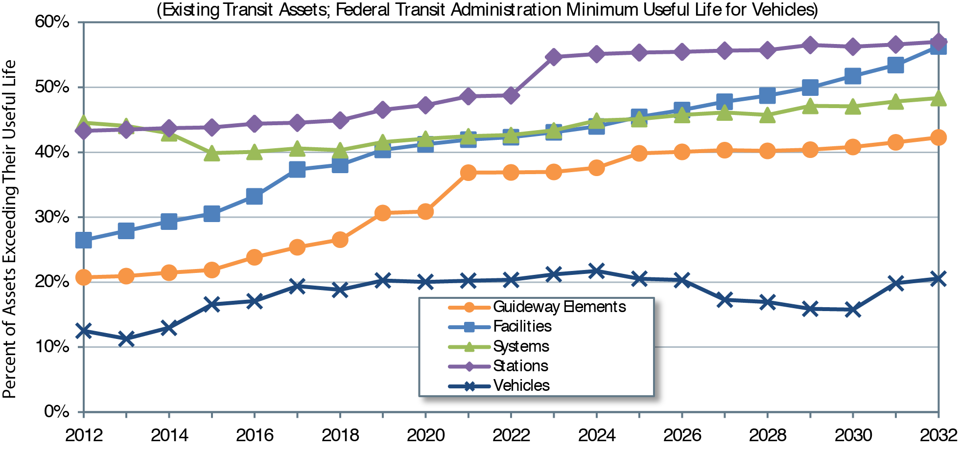
Note: The proportion of assets exceeding their useful life is measured based on asset replacement value, not asset quantities.
Source: Transit Economic Requirements Model.
Exhibit 8-17 Investment Backlog: Sustain 2012 Spending ($10 Billion Annually)
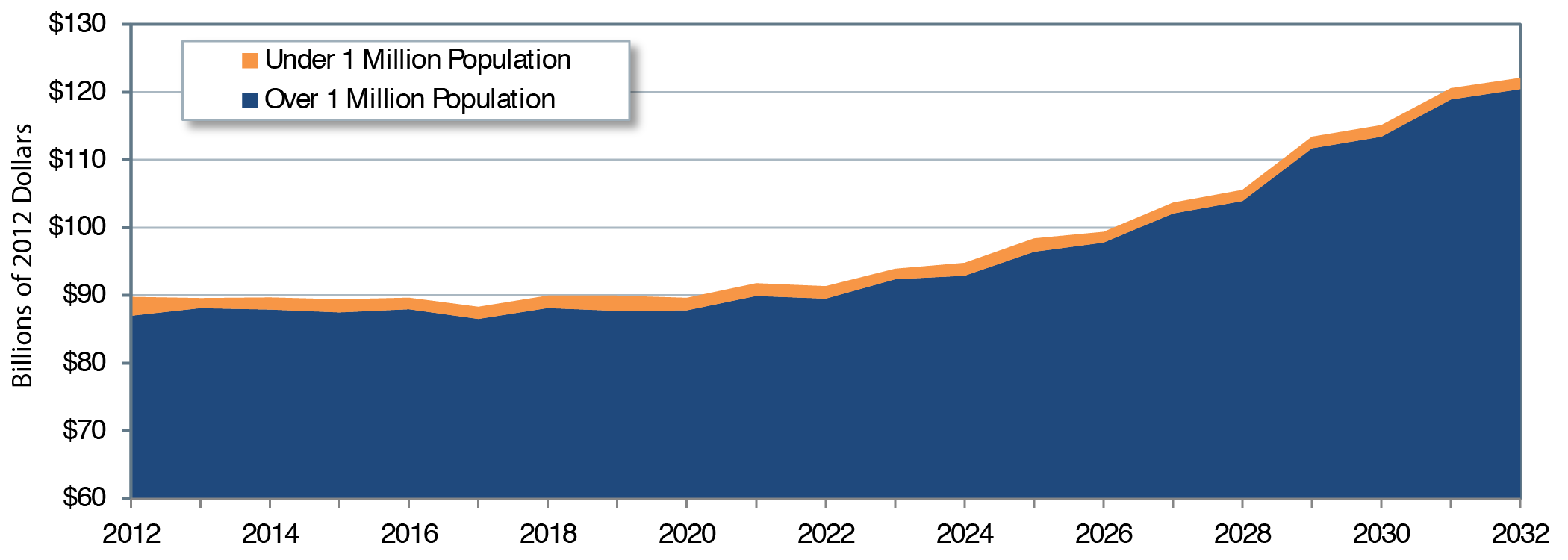
Source: Transit Economic Requirements Model.
The chart in Exhibit 8-17 also divides the backlog amount according to size of transit service area, with the lower portion showing the backlog for UZAs having populations greater than 1 million and the upper portion showing the backlog for all other UZAs and rural areas combined. This segmentation highlights the significantly higher existing backlog for those UZAs serving the largest number of transit riders. Regardless of the actual allocation, the 2012 expenditure level of $10.0 billion, if sustained, clearly is not sufficient to prevent a further increase in the backlog needs of one or more of these UZA types.
Expansion Investments
In addition to the $10.0 billion spent on preserving transit assets in 2012, transit agencies spent $7.1 billion on expansion investments to support ridership growth and improve transit performance. This section considers the impact of sustaining the 2012 level of expansion investment on future ridership capacity and vehicle utilization rates under the assumptions of both lower and higher growth rates in ridership (i.e., the Low-Growth and High-Growth scenarios). As noted above, recall that the $7.1 billion spent on expansion investments in 2012 was significantly higher than that reported in prior years.
As previously considered in Chapter 7 (see Exhibit 7-23), the 2012 rate of investment in transit expansion is not sufficient to expand transit capacity at a rate equal to the rate of growth in travel demand, as projected by the historical trend rate of increase. Under these circumstances, transit capacity utilization (e.g., passengers per vehicle) should be expected to increase, with the level of increase determined by actual growth in demand. Although the impact of this change could be minimal for systems that currently have lower-capacity utilization, service performance on some higher-utilization systems likely would decline as riders experience increased vehicle crowding and service delays. Exhibit 8-18 illustrates this potential impact. It presents the projected change in vehicle occupancy rates by mode from 2012 through 2032 (reflecting the impacts of spending from 2013 through 2032) under both the Low-Growth and High-Growth scenarios in transit ridership, assuming that transit agencies continue to invest an average of $7.1 billion per year on transit expansion. Under the Low-Growth scenario, capacity utilization-or the average number of riders per transit vehicle-decreases across each of the four modes depicted here, indicating that investment is sufficient or higher than needed to maintain current occupancy levels. For the High-Growth scenario, however, the average number of riders per transit vehicle steadily rises across each mode. Chapter 9 provides more detail on the new methodology for both the Low- and High-Growth scenarios.
Exhibit 8-18 Sustain 2012 Spending Scenario: Capacity Utilization by Mode Forecast, 2012—2032
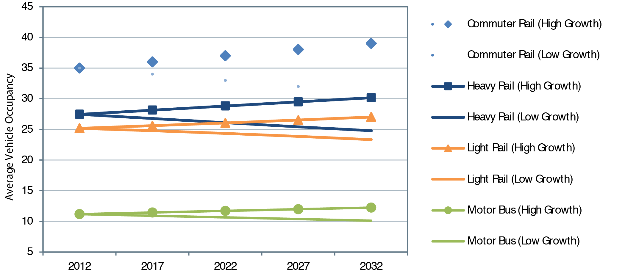
Source: Transit Economic Requirements Model.
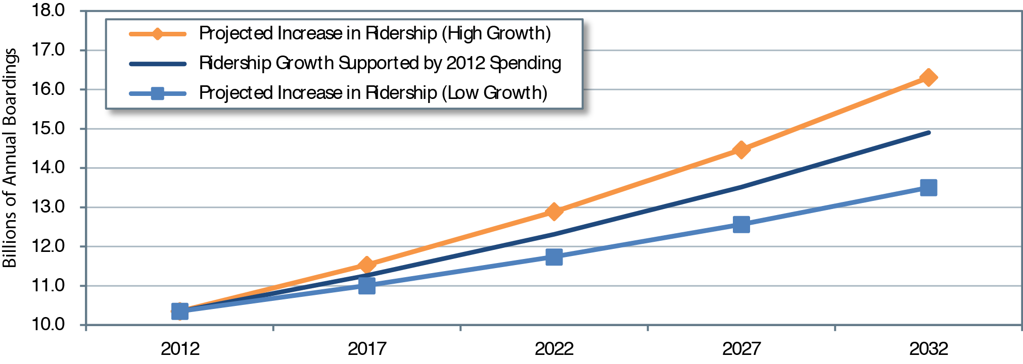
Exhibit 8-19 presents the projected growth in transit riders that the 2012 level of investment (keeping vehicle occupancy rates constant) can accommodate as compared with the potential growth in total ridership under both the Low-Growth and High-Growth scenarios. Similar to previous analyses, the $7.1-billion level of investment for expansion can support ridership growth that is similar to the ridership increases projected in the Low-Growth scenario, but is short of that required to support continued ridership under the High-Growth scenario (i.e., without impacting service performance).
Exhibit 8-19 Projected vs. Currently Supported Ridership Growth
Source: Transit Economic Requirements Model.
State of Good Repair Benchmark
The definition of "state of good repair" used for the SGR Benchmark relies on TERM's assessment of transit asset conditions. Specifically, for this benchmark, TERM considers assets to be in a state of good repair if they are rated at condition 2.5 or higher and if all required rehabilitation activities have been addressed.
The Sustain 2012 Spending scenario considered the impacts of sustaining transit spending at current levels, which appear to be insufficient to address either deferred investment needs (which are projected to increase) or the projected trends in transit ridership (without a reduction in service performance). In contrast, this section focuses on the level of investment required to eliminate the investment backlog over the next 20 years and to provide for sustainable rehabilitation and replacement needs once the backlog has been addressed. Specifically, the SGR Benchmark estimates the level of annual investment required to replace assets that currently exceed their useful lives, to address all deferred rehabilitation activities (yielding an SGR where the asset has a condition rating of 2.5 or higher), and to address all future rehabilitation and replacement activities as they come due. The SGR Benchmark considered here uses the same methodology as that described in FTA's National State of Good Repair Assessment, released June 2012.
Differences from Scenarios: In contrast to the scenarios described in this chapter, the SGR Benchmark does not (1) assess expansion needs or (2) apply TERM's benefit-cost test to investments proposed in TERM. These benchmark characteristics are inconsistent with the SGR concept. First, analyses of expansion investments ultimately focus on capacity improvements and not on the needs of deteriorated assets. Second, application of TERM's benefit-cost test would leave some potential reinvestment improvements unaddressed. The intention of this benchmark is to assess the total magnitude of unaddressed reinvestment needs for all transit assets currently in service, regardless of whether having these assets remain in service would be cost beneficial.
SGR Investment Needs
Annual reinvestment needs under the SGR Benchmark are presented in Exhibit 8-20. Under this benchmark, an estimated $ 17.0 billion in annual expenditures would be required over the next 20 years to bring the condition of all existing transit assets to an SGR. Of this amount, roughly $11.7 billion (69 percent ) is required to address the SGR needs of rail assets. Note that a large proportion of rail reinvestment needs are associated with guideway elements (primarily aging elevated and tunnel structures) and rail systems (including train control, traction power, and communications systems) that are past their useful lives and potentially are technologically obsolete. Bus-related reinvestment needs are primarily associated with aging vehicle fleets.
Exhibit 8-20 SGR Benchmark: Average Annual Investment by Asset Type, 2013 through 2032 |
|||
|---|---|---|---|
| Asset Type | Urban Area Type | Total | |
| Over 1 Million Population | Under 1 Million Population | ||
| (Billions of 2012 Dollars) | |||
| Rail | |||
| Guideway Elements | $3.2 | $0.1 | $3.2 |
| Facilities | $0.7 | $0.0 | $0.8 |
| Systems | $3.1 | $0.0 | $3.1 |
| Stations | $3.0 | $0.0 | $3.0 |
| Vehicles | $1.5 | $0.1 | $1.6 |
| Subtotal Rail1 | $11.5 | $0.2 | $11.7 |
| Nonrail | |||
| Guideway Elements | $0.1 | $0.0 | $0.1 |
| Facilities | $0.7 | $0.0 | $0.8 |
| Systems | $0.3 | $0.0 | $0.3 |
| Stations | $0.1 | $0.0 | $0.1 |
| Vehicles | $2.9 | $1.1 | $4.0 |
| Subtotal Nonrail1 | $4.1 | $1.2 | $5.3 |
| Total1 | $15.7 | $1.3 | $17.0 |
1 Note that totals may not sum due to rounding. Source: Transit Economic Requirements Model. |
|||
Exhibit 8-20 also provides a breakout of capital reinvestment needs by type of UZA. This breakout emphasizes the fact that capital reinvestment needs are most heavily concentrated in the Nation's larger UZAs. Together, these urban areas account for approximately 92 percent of total reinvestment needs (across all mode and asset types), with the rail reinvestment needs of these urban areas accounting for more than one-half the total reinvestment required to bring all assets to an SGR. This high proportion of total needs reflects the high level of investment in older assets found in these urban areas.
Impact on the Investment Backlog
A key objective of the SGR Benchmark is to determine the level of investment required to attain and then maintain an SGR across all transit assets over the next 20 years, including elimination of the existing investment backlog. Exhibit 8-21 shows the estimated impact of the $17.0 billion in annual expenditures under the SGR Benchmark on the existing investment backlog over the 20year forecast period (compare these data with Exhibit 8-17). Given this level of expenditures, the backlog is projected to be eliminated by 2032, with most of this drawdown addressing the reinvestment needs of the UZAs having populations greater than 1 million.
Exhibit 8-21 Investment Backlog: State of Good Repair Benchmark ($16.6 Billion Annually)
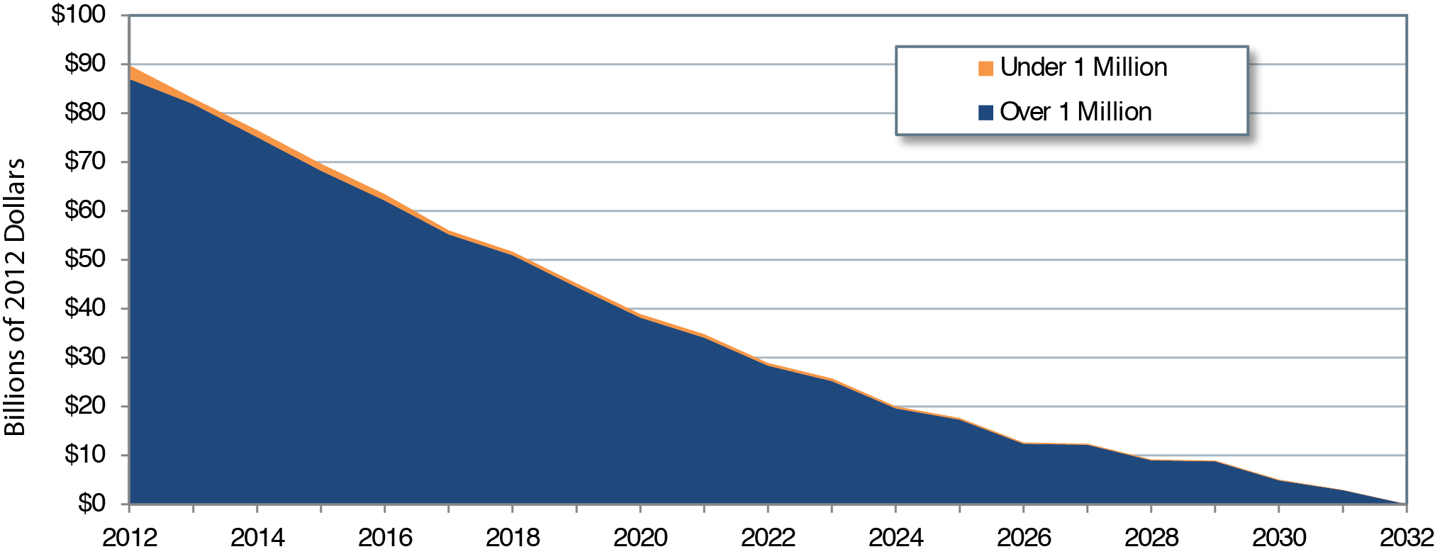
Source: Transit Economic Requirements Model.
Impact on Conditions
In drawing down the investment backlog, the annual capital expenditures of $17.0 billion under the SGR Benchmark also would lead to the replacement of assets with an estimated condition rating of 2.5 or less. Within TERM's condition rating system, these assets would include those in marginal condition having ratings less than 2.5 and all assets in poor condition. Exhibit 8-22 shows the current distribution of asset conditions for assets estimated to be in a rating condition of 2.5 or less (with assets in poor condition divided into two subgroups). Note that this graphic excludes both tunnel structures and subway stations in tunnel structures because these are considered assets that require ongoing capital rehabilitation expenditures but that are never actually replaced. As with the investment backlog, the proportion of assets at condition rating 2.5 or lower is projected to decrease under the SGR Benchmark from roughly 14 percent of assets in 2012 to less than 1 percent by 2032. Once again, this replacement activity would remove from service those assets with higher occurrences of service failures, technological obsolescence, and lower overall service quality. Important to note is that the assets with condition less than 2.5 presented in Exhibit 8-22 capture only a subset of assets in the SGR backlog as depicted in Exhibit 8-21. Specifically, the total SGR backlog (Exhibit 8-21) includes not just those assets in need of replacement (i.e., those at less than condition 2.5), but also those assets in need of rehabilitation or other form of capital reinvestment.
Exhibit 8-22 Proportion of Transit Assets Not in State of Good Repair (Excluding Tunnel Structures)
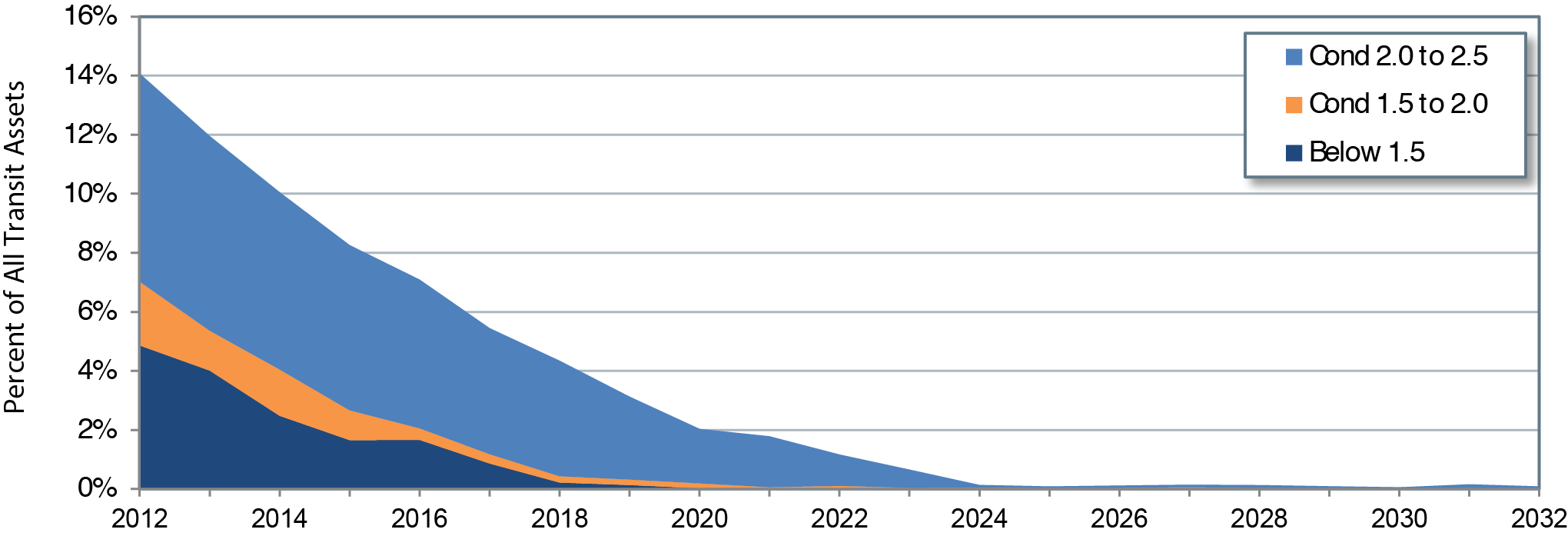
Source: Transit Economic Requirements Model.
Low-Growth and High-Growth Scenarios
The SGR Benchmark considered the level of investment to bring existing transit assets to an SGR but in doing so did not consider either (1) the economic feasibility of these investments (investments were not required to pass TERM's benefit-cost test) or (2) the level of expansion investment required to support projected ridership growth. The Low-Growth scenario and High-Growth scenario address both these issues. Specifically, these scenarios use the same rules to assess when assets should be rehabilitated or replaced as were applied in the preceding SGR Benchmark (e.g., with assets being replaced at condition 2.5), but also require that these preservation and expansion investments pass TERM's benefit-cost test. In general, some reinvestment activities do not pass this test (i.e., have a benefit-cost ratio less than 1), which can result from low ridership benefits, higher capital or operating costs, or a mix of these factors. Excluding investments that do not pass the benefit-cost test has the effect of reducing total estimated needs.
In addition, the Low- and High-Growth scenarios also assess transit expansion needs given ridership growth based on the average annual compound rate as experienced over the past 15 years minus 0.5 percent (Low-Growth) or plus 0.5 percent (High-Growth). For the expansion component of this scenario, TERM assesses the level of investment required to maintain current vehicle occupancy rates (at the agency-mode level) subject to the rate of projected growth in transit demand in that UZA and subject to the proposed expansion investment passing TERM's benefit-cost test.
Low- and High-Growth Assumptions
The Low-Growth scenario is intended to provide a lower bound on the level of investment required to maintain current service performance (as measured by transit vehicle capacity utilization) as determined by a relatively low rate of growth in travel demand. In contrast, the High-Growth scenario provides a higher bound on the level of investment required to maintain current service performance as determined by a relatively high rate of growth in travel demand. The methodology for the Low- and High-Growth scenarios has been revised to use a common, consistent approach that better reflects differences in PMT growth by mode. Specifically, these scenarios are now based on the 15-year trend rate of growth in PMT. When calculated across all transit operators and modes, this historical trend rate of growth converts to a national average compound annual growth rate of approximately 1.7 percent during the 20-year period.
Within this new framework, the Low-Growth scenario is defined as the trend rate of growth (by FTA region, population stratum, and mode) less 0.5 percent , while the High-Growth scenario is defined as the trend rate of growth plus 0.5 percent . Hence, the Low-Growth and High-Growth scenarios differ by a full 1.0 percent in annual growth.
Low- and High-Growth Scenario Needs
Exhibit 8-23 presents TERM's projected capital investment needs on an annual average basis under the Low- and High-Growth scenarios, including those for both asset preservation and asset expansion.
Exhibit 8-23 Low-Growth and High-Growth Scenarios: Average Annual Investment by Asset Type, 2013 through 2032 |
||||||
|---|---|---|---|---|---|---|
| Asset Type | Lower Growth | Total | Higher Growth | Total | ||
| Preservation | Expansion | Preservation | Expansion | |||
| (Billions of 2012 Dollars) | (Billions of 2012 Dollars) | |||||
| Rail | ||||||
| Guideway Elements | $3.2 | $1.2 | $4.4 | $3.2 | $1.7 | $4.9 |
| Facilities | $0.7 | $0.2 | $0.9 | $0.8 | $0.3 | $1.1 |
| Systems | $3.1 | $0.3 | $3.4 | $3.1 | $0.3 | $3.5 |
| Stations | $3.0 | $0.7 | $3.7 | $3.0 | $1.0 | $3.9 |
| Vehicles | $1.5 | $1.9 | $3.4 | $1.5 | $3.0 | $4.5 |
| Other Project Costs | $0.0 | $1.3 | $1.3 | $0.0 | $1.7 | $1.7 |
| Subtotal Rail1 | $11.6 | $5.5 | $17.1 | $11.6 | $7.9 | $19.5 |
| Subtotal UZAs Over 1 Million1 | $11.4 | $5.5 | $16.9 | $11.5 | $7.9 | $19.3 |
| Subtotal UZAs Under 1 Million and Rural1 | $0.1 | $0.03 | $0.2 | $0.2 | $0.04 | $0.2 |
| Nonrail | ||||||
| Guideway Elemen class="liteblue"ts | $0.1 | $0.0 | $0.1 | $0.1 | $0.0 | $0.1 |
| Facilities | $0.7 | $0.1 | $0.8 | $0.7 | $0.3 | $1.0 |
| Systems | $0.2 | $0.0 | $0.3 | $0.3 | $0.1 | $0.3 |
| Stations | $0.0 | $0.0 | $0.0 | $0.0 | $0.0 | $0.1 |
| Vehicles | $3.8 | $0.7 | $4.6 | $3.8 | $1.5 | $5.4 |
| Other Project Costs | $0.0 | $0.0 | $0.0 | $0.0 | $0.0 | $0.0 |
| Subtotal Nonrail1 | $4.9 | $0.9 | $5.8 | $4.9 | $2.0 | $6.9 |
| Subtotal UZAs Over 1 Million1 | $3.7 | $0.4 | $4.1 | $3.8 | $1.1 | $4.9 |
| Subtotal UZAs Under 1 Million and Rural1 | $1.1 | $0.5 | $1.7 | $1.1 | $0.9 | $2.0 |
| Total Investment1 | $16.4 | $6.4 | $22.9 | $16.5 | $9.9 | $26.4 |
| Total UZAs Over 1 Million1 | $15.2 | $5.9 | $21.1 | $15.2 | $9.0 | $24.2 |
| Total UZAs Under 1 Million and Rural1 | $1.3 | $0.5 | $1.8 | $1.3 | $0.9 | $2.2 |
1 Note that totals may not sum due to rounding. Source: Transit Economic Requirements Model. | ||||||
Lower-Growth Needs
Assuming the relatively low ridership growth in the Low-Growth scenario, investment needs for system preservation and expansion are estimated to average roughly $22.9 billion each year for the next two decades. Of this amount, roughly 72 percent is for preserving existing assets and approximately $11.6 billion is associated with preserving existing rail infrastructure alone. Note that the $0.6billion difference between the $17.0 billion in annual preservation needs under the SGR Benchmark and the $16.4 billion in preservation needs under the Low-Growth scenario is entirely due to the application of TERM's benefit-cost test under the Low-Growth scenario. Finally, expansion needs in this scenario total $6.4 billion annually, with 86 percent of that amount associated with rail expansion costs.
Higher-Growth Needs
In contrast, total investment needs under the High-Growth scenario are estimated to be $26.4 billion annually, a 15-percent increase over the total investment needs under the Low-Growth scenario. The High-Growth scenario total includes $16.5 billion for system preservation and an additional $9.9 billion for system expansion. Note that system preservation costs are higher under the High-Growth scenario because the higher growth rate leads to a larger expansion of the asset base as compared to the Low-Growth scenario. Under this scenario, investment in expansion of rail assets is still larger than that for nonrail expansion (80 percent for rail and 20 percent for nonrail). Under the High-Growth scenario, however, rail takes only 80 percent of total expansion investment versus 86 percent of expansion needs under the Low-Growth scenario.
Impact on Conditions and Performance
The impact of the Low- and High-Growth rate preservation investments on transit conditions is essentially the same as that already presented for the SGR Benchmark in Exhibits 8-21 and 8-22. As noted above, the Low and High-Growth scenarios use the same rules to assess when assets should be rehabilitated or replaced as were applied in the SGR Benchmark (e.g., with assets being replaced at condition rating 2.5). In terms of asset conditions, the primary difference between the SGR Benchmark and the Low- and High-Growth scenarios relates to (1) TERM's benefit-cost test not applying to the SGR Benchmark (leading to higher SGR preservation needs overall) and (2) the Low- and High-Growth scenarios having some additional needs for replacing expansion assets with short service lives. Together, these impacts tend to work in opposite directions. The result is that the rate of drawdown in the investment backlog and the elimination of assets exceeding their useful lives are roughly comparable between the SGR Benchmark and these scenarios and between the two scenarios.
Similarly, the impact of the Low- and High-Growth rate expansion investments on transit ridership was considered in Exhibit 8-19. That analysis demonstrated the significant difference in the level of ridership growth supported by the High-Growth scenario as compared with either the current level of expenditures ($6.6 billion in 2012 for UZAs with populations greater than 1 million) or the rate of growth supported under the Low-Growth scenario.
Scenario Impacts Comparison
Finally, this subsection summarizes and compares many of the investment impacts associated with each of the three analysis scenarios and the SGR Benchmark considered above. Although much of this comparison is based on measures already introduced above, this discussion also considers a few additional investment impact measures. These comparisons are presented in Exhibit 8-24. Note that the first column of data in Exhibit 8-24 presents the current values for each of these measures (as of 2012). The subsequent columns present the estimated future values in 2032, assuming the levels, allocations, and timing of expenditures associated with each of the three investment scenarios and the SGR Benchmark.
Exhibit 8-24 includes the following measures:
- Average annual expenditures (billions of dollars): This amount is broken down into preservation and expansion expenditures.
- Condition of existing assets: This analysis considers only the impact of investment funds on the condition of those assets currently in service.
Average physical condition rating: The weighted average condition of all existing assets on TERM's condition scale of 5 (excellent) through 1 (poor).
Investment backlog:The value of all deferred capital investment, including assets exceeding their useful lives and rehabilitation activities that are past due (this value can approach but never reach zero due to assets continually aging with some exceeding their useful lives). The backlog is presented here both as a total dollar amount and as a percent of the total replacement value of all U.S. transit assets.
Backlog ratio: The ratio of the current investment backlog to the annual level of investment required to maintain normal annual capital needs once the backlog is eliminated.
- Performance measures: The impact of investments on U.S. transit ridership capacity and system reliability.
New boardings supported by expansion investments: The number of additional riders that transit systems can carry without a loss in performance (given the projected ridership assumptions for each scenario).
Revenue service disruptions per PMT: Number of disruptions to revenue service per million passenger miles.
Fleet maintenance cost per vehicle revenue mile: Fleet maintenance costs tend to increase with fleet age (or reduced asset condition). This measure estimates the change in fleet maintenance costs expressed in a per-revenue-vehicle-mile basis.
Exhibit 8-24 Scenario Investment Benefits Scorecard |
|||||
|---|---|---|---|---|---|
| Measure | Baseline 2012 Actual Spending, Conditions and Performance | Projections for 2032 | |||
| SGR Benchmark | Sustain 2012 Spending Scenario | Low-Growth Scenario | High-Growth Scenario | ||
| Average Annual Expenditures (Billions of 2012 Dollars) | |||||
| Preservation | $9.9 | $17.0 | $9.9 | $16.4 | $16.5 |
| Expansion | $7.1 | NA | $7.1 | $6.4 | $9.9 |
| Total | $17.0 | $17.0 | $17.0 | $22.8 | $26.4 |
| Conditions (Existing Assets) | |||||
| Average Physical Condition Rating | 3.5 | 3.2 | 3.1 | 3.4 | 3.6 |
| Investment Backlog (Billions of Dollars) | $89.8 | $0.0 | $121.7 | $0.0 | $0.0 |
| Investment Backlog (% of Replacement Costs) | 10.6% | 0.0% | 14.4% | 0.0% | 0.0% |
| Backlog Ratio1 | 7.2 | 0.0 | 9.7 | 0.0 | 0.0 |
| Performance | |||||
| Ridership Impacts of Expansion Investments (2012) | |||||
| New Boardings Supported by Expansion (Billions) | NA | NA | 3.4 | 3.1 | 5.8 |
| Total Projected Boardings in 2032 (Billions) | NA | NA | 13.7 | 13.5 | 16.2 |
| Fleet Performance | |||||
| Revenue Service Disruptions per Thousand PMT | 8.0 | 8.2 | 8.0 | 8.2 | 8.2 |
| Fleet Maintenance Cost per Revenue Vehicle Mile | $1.83 | $1.85 | $1.81 | $1.84 | $1.85 |
1 The backlog ratio is the ratio of the current investment backlog to the annual level of investment to maintain SGR once the backlog is eliminated. Source: Transit Economic Requirements Model. | |||||
Scorecard Comparisons
A review of the scorecard results for each of the three investment scenarios and the SGR Benchmark reveals the impacts discussed below.
Preservation Impacts
Continued reinvestment at the 2012 level is likely to yield a decline in overall asset conditions (from 3.5 in 2012 to 3.1 in 2032) and an increase in the size of the investment backlog (from $89.8 billion in 2012 to $121.7 billion in 2032). Continued reinvestment at the 2012 level, however, likely will cause no change in service disruptions per million passenger miles and a decrease in maintenance costs per vehicle revenue mile. In contrast, with the exception of overall asset conditions, opposite results occur under the SGR Benchmark, the Low-Growth scenario, and the High-Growth scenario. Note that the overall condition rating measures of 3.2, 3.4, and 3.6 under the SGR Benchmark, the Low-Growth scenario, and the High-Growth scenario, respectively, represent sustainable, long-term condition levels for the Nation's existing transit assets over the long term. This is in contrast to the current measure of roughly 3.5, which would be difficult to maintain over the long term without replacing many asset types prior to the conclusion of their expected useful lives.
For this report, expansion assets are included in the overall condition rating measures. This approach is a departure from that in previous reports, in which the goal was to be cognizant of what happens to the SGR of existing assets under alternative scenarios.
Expansion Impacts
Although continued expansion investment at the 2012 level appears sufficient to support a low rate of increase in transit ridership to about 3.4 billion new boardings in 2032, higher rates of growth to nearly 5.8 billion new boardings in 2032 suggest that a significantly higher rate of expansion investment (nearly $3 billion more annually in expansion investment) is required to avoid a decline in overall transit performance (e.g., in the form of increased crowding on high-utilization systems).