

chapter 9
Highway Supplemental Scenario Analysis
Comparison of Scenarios with Previous Reports
Comparison With 2013 C&P Report
Comparisons of Implied Funding Gaps
Highway Travel Demand Forecasts
New National VMT Forecasting Model
Comparison of FHWA-Modeled Forecasts and HPMS Forecasts
VMT Forecasts from Previous C&P Reports
Alternative Timing of Investment in HERS
Alternative Timing of Investment in NBIAS
Transit Supplemental Scenario Analysis
Revised Method for Estimating PMT Growth Rates
Impact of New Technologies on Transit Investment Needs
Impact of Compressed Natural Gas and Hybrid Buses on Future Needs
Forecasted Expansion Investment
Highway Supplemental Scenario Analysis
This chapter explores the implications of the highway investment scenarios considered in Chapter 8, starting with a comparison of the scenario investment levels to those presented in previous C&P reports. This section also examines the long-term forecasts of vehicle miles traveled (VMT) presented in earlier C&P reports and compares them to actual outcomes. The highway travel demand forecast by the Highway Performance Monitoring System (HPMS) is also compared with FHWA-modeled forecasts to ensure consistency.
This chapter illustrates the impact of alternative rates of future inflation on the constant-dollar scenario investment levels presented in Chapter 8 and explores alternative assumptions about the timing of investment over the 20-year analysis period. A subsequent section within this chapter provides supplementary analysis regarding the transit investment scenarios.
Comparison of Scenarios with Previous Reports
Each edition of this report presents various projections of travel growth, pavement conditions, and bridge conditions under different performance scenarios. The projections cover 20-year periods, beginning the first year after the data presented on current conditions and performance. Although the scenario names and criteria have varied over time, the C&P report traditionally has included highway investment scenarios corresponding in concept to the Maintain Conditions and Performance scenario and the Improve Conditions and Performance scenario presented in Chapter 8.
Comparison With 2013 C&P Report
One obvious difference between the scenarios presented in this 2015 C&P Report and those in the 2013 C&P Report is that they cover a different 20-year period, 2013 through 2032 rather than 2011 through 2030. The 2013 edition also presented two alternative estimates for each scenario based on different assumptions regarding future travel growth, while the current edition reverts to the traditional approach of reporting only one primary estimate for each scenario, accompanied by sensitivity analyses presented in Chapter 10 that explore the impacts of alternative future travel growth rates.
Aside from these differences, the procedure used to determine the investment levels associated with the Improve Conditions and Performance scenario is the same for both editions. This scenario sets a level of spending sufficient to gradually fund all potential highway and bridge projects that are cost-beneficial over 20 years. Neither the 2013 C&P Report nor this 2015 C&P Report made assumptions about financing mechanisms that would be used to cover the costs of this scenario.
The Maintain Conditions and Performance scenario identifies a level of investment associated with keeping overall conditions and performance in 20 years at base-year levels. As discussed in Chapter 8, the target of the scenario component derived from the National Bridge Investment Analysis System (NBIAS) has been modified to maintain the percentage of total bridge deck area classified as structurally deficient or functionally obsolete, rather than to maintain the average bridge sufficiency rating as in the 2013 C&P Report. The target measures for the component of this scenario derived from the Highway Economic Requirements System (HERS)-average pavement roughness and average delay per VMT-were retained in the current edition but applied in a different way. Rather than following the 2013 C&P Report approach of taking the average of the annual investment levels predicted to be adequate for maintaining each of these two indicators, the scenario in the current edition was based on the higher of the two investment levels. Thus, under the new approach, the HERS component of the scenario reflects the lowest average level of investment at which both pavement roughness and delay either stay the same or improve.
As discussed in Chapter 6, highway construction costs are measured by the Federal Highway Administration's (FHWA's) National Highway Construction Cost Index, which increased by 6.1 percent between 2010 and 2012. Consequently, adjusting the 2013 C&P Report's scenario figures from 2010 dollars to 2012 dollars causes the observed and projected highway construction costs to appear larger. As shown in Exhibit 9-1, the 2013 C&P Report estimated the average annual investment level in the current Maintain Conditions and Performance scenario to range from $65.3 to $86.3 billion in 2010 dollars; adjusting for inflation shifts this range to $69.3 to $91.6 billion in 2012 dollars. The comparable amount for the Maintain Conditions and Performance scenario presented in Chapter 8 of this edition is $89.9 billion in 2012 dollars, approximately 1.9 percent lower than the high end of 2013 C&P Report estimate of $91.6 billion dollars.
Exhibit 9-1 Selected Highway Investment Scenario Projections Compared with Comparable Data from the 2013 C&P Report |
|||
|---|---|---|---|
| Highway and Bridge Scenarios-All Roads | 2011 Through 2030 Projection(Based on 2010 Data)1 | 2013 Through 2032 Projection(Billions of 2012 Dollars) | |
| 2013 C&P Report(Billions of 2010 Dollars) | Adjusted for Inflation2 (Billions of 2012 Dollars) | ||
| Maintain Conditions and Performance scenario3 | $65.3—$86.3 | $69.3—$91.6 | $89.9 |
| Improve Conditions and Performance scenario | $123.7—$145.9 | $131.3—$154.9 | $142.5 |
1 The 2013 C&P report included two alternative estimates for each scenario based on different assumptions regarding future travel growth. 2 The investment levels for the highway and bridge scenarios were adjusted for inflation using the FHWA National Highway Construction Cost Index. 3 In the 2013 C&P Report, the HERS component of this scenario focused on maintaining a composite indicator reflecting average delay and average pavement condition rather than just maintaining average pavement condition; the NBIAS component of the scenario focused on maintaining the average sufficiency rating for bridges rather than the percentage of deck area on deficient bridges. | |||
The average annual investment level in the 2013 C&P Report scenario comparable to the current Improve Conditions and Performance scenario was estimated to be $123.7 to $145.9 billion in 2010 dollars; adjusting for inflation increases this range to $131.3 to $154.9 billion in 2012 dollars. The comparable amount for the current Improve Conditions and Performance scenario presented in Chapter 8 of this edition is $142.5 billion, approximately 8.0 percent lower than the high end of 2013 C&P Report estimate of $154.9 billion dollars.
The changes in the scenario findings in this report relative to the 2013 C&P Report are also partially attributable to changes in the underlying characteristics, conditions, and performance of the bridge system reported in Chapters 2 and 3 and to changes in the analytical methodology and data in HERS and NBIAS. Despite changes in database and model specifications, the estimated investment needs suggest similar patterns for comparable scenarios over different editions of the C&P report.
Comparisons of Implied Funding Gaps
Exhibit 9-2 compares the funding gaps implied by the analysis in the current report with those implied by previous C&P report analyses. The funding gap is measured as the percentage by which the estimated average annual investment needs for a specific scenario exceeds the base-year level of investment. The scenarios examined are this report's Maintain Conditions and Performance scenario and Improve Conditions and Performance scenario, and their counterparts in previous C&P reports.
Exhibit 9-2 Comparison of Average Annual Highway and Bridge Investment Scenario Estimates with Base-Year Spending, 1997 to 2015 C&P Reports |
||||
|---|---|---|---|---|
| Report Year | Relevant Comparison | percent Above Base-Year Spending | ||
| Primary "Maintain" Scenario1 | Primary "Improve" Scenario1 | |||
| 1997 | Average annual investment scenario estimates for 1996 through 2015 compared with 1995 spending | 21.0% | 108.9% | |
| 1999 | Average annual investment scenario estimates for 1998 through 2017 compared with 1997 spending | 16.3% | 92.9% | |
| 2002 | Average annual investment scenario estimates for 2001 through 2020 compared with 2000 spending | 17.5% | 65.3% | |
| 2004 | Average annual investment scenario estimates for 2003 through 2022 compared with 2002 spending | 8.3% | 74.3% | |
| 2006 | Average annual investment scenario estimates for 2005 through 2024 compared with 2004 spending | 12.2% | 87.4% | |
| 2008 | Average annual investment scenario estimates for 2007 through 2026 compared with 2006 spending | 34.2% | 121.9% | |
| 2010 | Average annual investment scenario estimates for 2009 through 2028 compared with 2008 spending | 10.8% | 86.6% | |
| 2013 | Average annual investment scenario estimates for 2011 through 2030 compared with 2010 spending | -13.9% | 45.7% | |
| 2015 | Average annual investment scenario estimates for 2013 through 2032 compared with 2012 spending | -14.6% | 35.5% | |
1 Amounts shown correspond to the primary investment scenario associated with maintaining or improving the overall highway system in each C&P report; the definitions of these scenarios are not fully consistent among reports. The values shown for this report reflect the Maintain Conditions and Performance and the Improve Conditions and Performance scenarios. Negative numbers signify that the investment scenario estimate was lower than base-year spending. Sources: Highway Economic Requirements System and National Bridge Investment Analysis System. | ||||
Prior to the 2013 C&P Report, each C&P report edition showed that actual annual spending in the base year for that report had been below the estimated average investment level required to maintain conditions and performance at base-year levels over 20 years. In both the 2013 C&P Report and this 2015 C&P Report, the trend was reversed and gaps between actual and required amounts for the primary "Maintain" scenario (the higher VMT growth scenario in 2013 C&P Report) became negative. This result dramatically differs from the positive numbers estimated in pre-2013 C&P reports, indicating that base-year spending reported in the 2013 and 2015 C&P Reports was more than the average annual spending levels identified for the Maintain Conditions and Performance scenario. The primary "Improve" scenario follows a similar trend, where the funding gap has dropped steadily since its peak in the 2008 C&P Report.
Changes in actual capital spending by all levels of government combined can substantially alter these spending gaps, as can sudden, large swings in construction costs. The large increase in the gap between base-year spending and the primary Maintain and Improve scenarios presented in the 2008 C&P Report coincided with a large increase of construction costs experienced between 2004 and 2006 (base year for the 2008 C&P Report). On the other hand, the decreases in the gaps presented in recent editions coincided with declines in construction costs since their 2006 peak.
The differences among C&P report editions in the implied gaps reported in Exhibit 9-2 are not a consistent indicator of change over time in how effectively highway investment needs are addressed. FHWA continues to enhance the methodology used to determine scenario estimates for each edition of the C&P report to provide a more comprehensive and accurate assessment. In some cases, these refinements have increased the level of investment in one or both of the scenarios (the Maintain or Improve scenarios, or their equivalents); other refinements have reduced this level.
Highway Travel Demand Forecasts
For each HPMS sample highway section, States provide the actual traffic volume in the base year and a forecast of traffic volume for a future year, typically 20 years after the base year. The HPMS reporting guidance requires the traffic forecasts States generate to be derived from a technically supportable procedure based on available information concerning the particular section and corridor to which it belongs. Because the HERS model was introduced in the 1995 C&P Report and used through the 2010 C&P Report, the primary highway investment scenarios presented in each of these editions relied on these State-provided forecasts. Without specific information regarding the assumptions built into the State forecasting procedures, an assumption was made that the forecasts reflected the level of future VMT that would occur for each HPMS sample section if average user costs, including costs of travel time, vehicle operation, and crash risk, were unchanged over the 20-year analysis period. Beginning with the 1999 C&P Report, sensitivity analyses also were presented showing the implications of alternative rates of future VMT growth. The sensitivity analysis was conducted by using the State-reported values for individual sample sections as a starting point. The values then were adjusted upward or downward proportionally, as needed to achieve a particular nationwide level of VMT growth.
The 2013 C&P Report followed the same general approach, except that it presented two alternative sets of scenarios. One scenario was based on the State-provided HPMS forecasts. For the other scenario, these forecasts were proportionally adjusted downward to match the average annual VMT growth rate observed over the preceding 15 years.
The primary advantage of using the State-provided VMT forecasts in the baseline analysis derives from their geographic specificity. Separate forecasts are provided for more than 100,000 HPMS sample sections. States can account for local conditions of a specific section and project long-term travel patterns of the particular routes or corridors accordingly. These section-level forecasts enable more refined projections of future travel demand.
The primary disadvantage of relying solely on the State-provided VMT forecasts is the uncertainty about exactly what they represent. To the extent that some States factor in changes to components of highway user costs in making their predictions, the traditional assumption made in HERS-that these are "constant-price" forecasts that do not reflect such changes-would be incorrect. Thus, the travel demand elasticity procedures in HERS discussed in Chapter 7, which adjust future VMT projections based on changes in "price" of travel as reflected by user costs, could be double counting the effects of some changes. Also, although the forecasts supplied for individual HPMS sample sections might appear reasonable in isolation based on information available at that particular location, when aggregated with all other forecasts for a given State or nationally, they could yield an overall growth rate that appears inconsistent with observed trends.
To address these issues, FHWA has adopted a new national-level VMT forecasting model. The analyses presented in this 2015 C&P Report used State-provided VMT forecasts for highways and bridges in HERS and NBIAS, respectively, as the starting point. Then, these values were proportionally reduced to yield a national-level forecast consistent with the predictions of this new VMT forecasting model. HERS also was modified to account for changes in user costs built into the VMT forecasts when applying its travel demand elasticity procedures to avoid three potential issues: (1) double counting the effects of assumed constant-dollar increases in the value of time, (2) presumed changes in constant-dollar fuel prices, and (3) changes in the share of total travel attributable to single-unit and combination trucks.
New National VMT Forecasting Model
The Volpe National Transportation Systems Center developed the National Vehicle Miles Traveled Projection for FHWA. The first projection was released in May 2014. The documentation for the model version used for this forecast is posted at http://www.fhwa.dot.gov/policyinformation /tables/vmt/vmt_model_dev.cfm . The current plan is to release revised forecasts each May; this 2015 C&P Report relies on the 20-year forecasts for the Baseline Economic Outlook from the May 2015 release posted at http://www.fhwa.dot.gov/policyinformation/tables/vmt/vmt_forecast _sum.cfm.
The travel forecasting model estimates future changes in passenger and freight VMT based on predicted changes in demographic and economic conditions. Built on economic theory, the national total VMT model establishes a separate but structurally similar econometric model for each of three vehicle categories-light-duty vehicles, single-unit trucks, and combination trucks using time series data beginning in the 1960s. These econometric models include underlying factors that strongly influence user demand to travel, such as demographic characteristics, economic activity, employment, cost of driving, road miles, and transit service availability. The three econometric models are applied to different roadway classes to develop detailed forecasts of future travel demand and VMT growth. A separate model is used for national-level bus VMT.
In addition to the econometric approaches used to construct the aggregate national VMT models, the travel forecasting models include a methodology for forecasting national VMT from a vehicle fleet perspective. This component of the VMT models disaggregates nationwide total VMT by vehicle class, model year or vintage, and vehicle age. The aggregate national-level VMT totals for each vehicle type were estimated and used as control totals for lower-level (functional classification and location) models. The econometric and vehicle fleet approaches are complementary and provide a more accurate forecast of future VMT.
Comparison of FHWA-Modeled Forecasts and HPMS Forecasts
Based on the May 2015 release, the FHWA forecast for the Baseline Economic Outlook is for VMT to grow at an average annual rate of 1.04 percent per year. In contrast, aggregating the forecasts for individual HPMS sample sections yields a composite, weighted-average, annual VMT growth rate between the 2012 base year and the forecast year, 2032, of 1.41 percent .
Exhibit 9-3 translates these two average annual VMT growth rates into projected annual VMT for each year from 2012 to 2032 for Federal-aid highways and for all roads combined. Consistent with the approach used in the HERS and NBIAS analyses for this report and other recent editions of the C&P report, future VMT is assumed to grow linearly (so that 1/20th of the additional VMT is added each year), rather than geometrically (growing at a constant annual rate). With linear growth, the annual percentage rate of growth gradually declines over the forecast period. This approach is logically consistent with the FHWA national VMT forecasting model, which projects lower average annual VMT growth rates over 30 years than it does over 20 years.
The VMT on all roads in 2012 was estimated at 2.99 trillion, and by 2032, VMT would reach 3.67 trillion, assuming an average annual VMT growth rate of 1.04 percent per year. The investment analyses presented in Chapters 7 and 8 reflect this assumption. Exhibit 9-3 also projects that VMT on Federal-aid highways will rise from 2.53 trillion to 3.11 trillion by 2032; these are the values actually modeled in HERS, as it considers only Federal-aid highways.
If future VMT were to rise at an average annual rate of 1.41 percent , consistent with the weighted aggregate VMT growth rate derived from the State-provided HPMS forecasts, total VMT would rise to 3.95 trillion by 2032, with 3.34 trillion VMT occurring on Federal-aid highways. Aggregating the forecasts of future bridge traffic reported in the National Bridge Inventory yields a similar average annual growth rate of 1.46 percent . Chapter 10 includes a sensitivity analysis showing how substituting these State-supplied forecasts would affect the projection of the Maintain Conditions and Performance scenario and the Improve Conditions and Performance scenario presented in Chapter 8.
Exhibit 9-3 Annual Projected Highway VMT Based on HPMS-Derived Forecasts or FHWA VMT Forecast Model
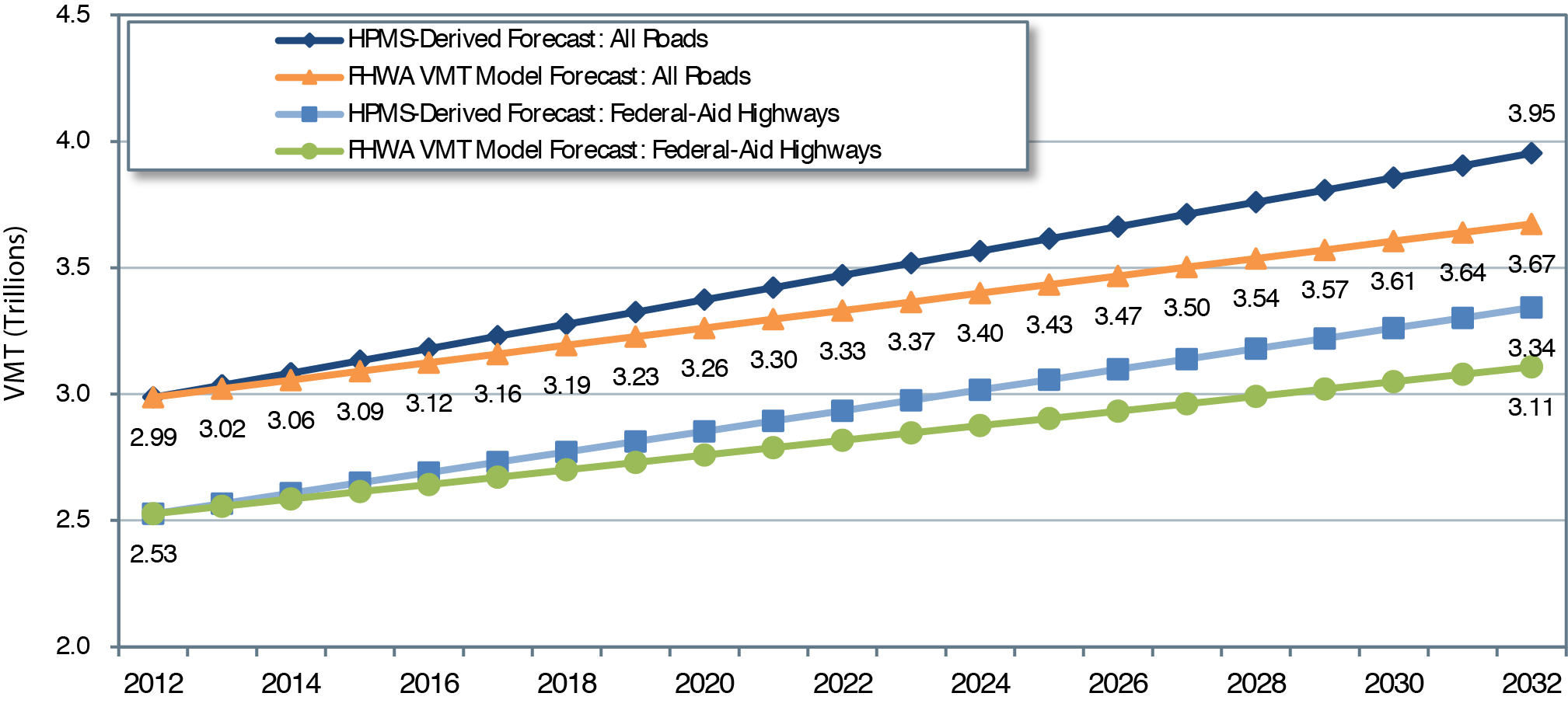
Sources: Highway Performance Monitoring System; FHWA Forecasts of Vehicle Miles Traveled (VMT), May 2015.

The United States recorded 2.99 trillion vehicle miles traveled (VMT) in 2012. According to preliminary statistics of the Federal Highway Administration, annual VMT is estimated to have increased by 0.6 percent in 2013, 1.7 percent in 2014, and 3.5 percent in 2015 to a level of 3.15 trillion.
A wide variety of factors correlate with the VMT trend, including macroeconomic and demographic factors and the availability of other transportation modes. Key economic variables that contribute to an increase in VMT are a declining unemployment rate and increasing income. Drivers respond to changes in fuel prices, and lower gas prices encourage more discretionary driving. Demographic changes also might explain the development of VMT. For example, a growing population tends to drive more. Other forces also can decrease VMT: The younger generation takes fewer automobile trips, and options to telecommute decrease travel demand.
VMT Forecasts from Previous C&P Reports
Future traffic projection is central to evaluations of capital spending on transportation infrastructure. Forecasting future traffic conditions, however, is extremely difficult because many uncertain circumstances are related to travel behavior. A rich body of literature has examined the accuracy issue of travel demand modeling and found rampant inaccuracy in project-specific traffic forecasts, with most at least 20—30 percent off actual future traffic volumes (see Flyvbjerg, Holm, and Buhl [2005] and Hartgen [2013], for example). This inaccuracy could be attributable to the model's failure to consider influencing factors (e.g., changing demographics and preferences), the effects of certain policies (e.g., pedestrian and bicycle), or treating changes in VMT growth patterns as temporary phenomena instead of long-term trends. These project-level inaccuracies could translate into inaccuracy in national aggregates. Even where the underlying relationships may be correctly modeled, the evolution of key variables (such as expected regional economic growth) could differ significantly from the assumptions made in the VMT forecast.
In light of this uncertainty, that the effective VMT growth rates predicted in the C&P report could be off target is not surprising. Exhibit 9-4 presents the long-term VMT projections in the 21 C&P reports starting in 1968, including the current report, and compares them to actual highway VMT. The forecasts differed from actual trends in most cases, sometimes underestimating future travel demand and other times overestimating it.
Each of the first five editions of the C&P report (1968 through 1977) underpredicted future total VMT by about 10 to 15 percent . Actual VMT for periods covered by these forecasts grew by more than 3 percent per year; in contrast, the average annual VMT growth rate forecasts among these five editions ranged from 2.2 to 2.7 percent .
The total VMT forecasts in the next five editions of the C&P report (1981 through 1989) were closer to the mark, deviating from actual VMT for the forecast periods by plus or minus 5 percent . The highest annual VMT growth forecast presented in the C&P report series was 2.85 percent per year from 1985 to 2000, presented in the 1987 C&P Report; VMT actually grew slightly faster during this period, increasing at an average annual rate of 2.95 percent . The 1989 C&P Report came the closest to projecting future VMT accurately, as the report's forecast of 3.05 trillion VMT in 2007 was within 0.66 percent of actual 2007 VMT of 3.03 trillion; the average annual VMT growth rate forecast in this edition was 2.34 percent , while VMT actually grew by 2.31 percent over this period.
The next two editions of the C&P report (1991 and 1993) are the last for which the 20-year projection period ended by 2012. Both significantly overpredicted future total VMT, by 16 to 21 percent . Both reports projected annual VMT growth of approximately 2.5 percent per year, but actual VMT growth during their forecast periods had fallen to well below 2 percent per year.
Although the 20-year forecast period for the 1995 C&P Report and later editions had not yet concluded by the end of 2012, each appears to be overpredicting future VMT so far, by about 1 to 2 percent per year. States have gradually reduced their projections of future annual VMT growth, but these reductions have not kept pace with recent declines in the actual rates of VMT growth.
Exhibit 9-4 illustrates that States tended to underpredict future VMT when actual VMT was growing rapidly and to overpredict when actual VMT growth stagnated or declined. This observation suggests that many States have been slow to adjust their models to incorporate emerging socioeconomic trends, as they wait to determine whether new data observations represent one-time phenomena or the start of new long-term trends. The downward shift in the VMT forecasts the States provided as part of the 2012 HPMS submittal was significant, as were the further reductions applied in HERS and NBIAS for this 2015 C&P Report to match the predictions of the new FHWA VMT forecasting model. Had the 1.42-percent-per-year VMT growth rate derived from the 2012 HPMS data been used for this report, it would have been the lowest rate assumed during the C&P report series; the further reduction to the 1.04-percent VMT growth rate assumed in Chapters 7 and 8 represents an even more significant departure from the forecasts in previous reports. Actual VMT growth over the next several years will help inform whether these changes have gone too far or have not gone far enough. The findings presented in Exhibit 9-4 emphasize that, given the uncertainties involved, considering the implications of the sensitivity analyses presented in Chapter 10 rather than focusing purely on the summary findings presented in Chapter 8 is essential.
Exhibit 9-4 State-Provided Long-Term VMT Forecasts Compared with Actual VMT, 1965—20321
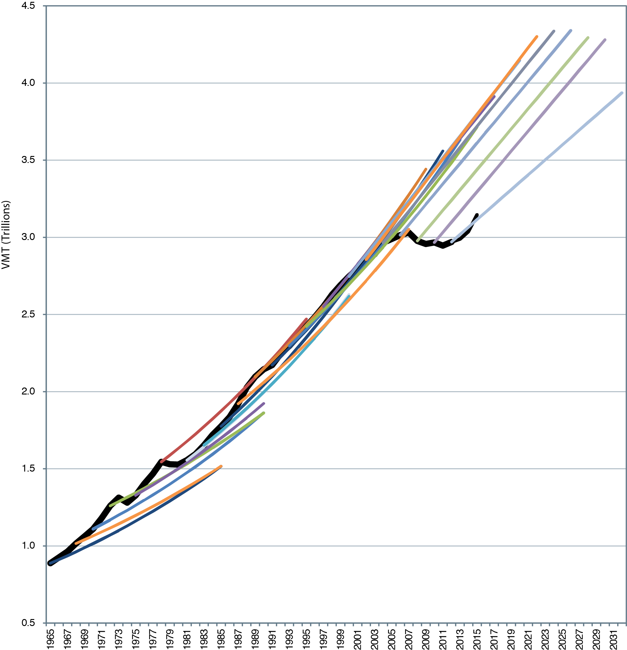
1Solid black line represents actual VMT through 2012; dashed black line reflects preliminary estimates through 2015. Other dashed lines represent State-provided long-term VMT forecasts utilized in the C&P report; since 1980, these have been derived from the HPMS.
Source: C&P Report, various years.
Timing of Investment
The investment-performance analyses presented in this report focus mainly on how alternative average annual investment levels over 20 years might impact system performance at the end of this period. Within this period, the timing of investment can significantly influence system performance. The discussion below explores the impacts of three alternative assumptions about the timing of future investment-baseline ramped spending, flat spending, or spending driven by benefit-cost ratio (BCR)-on system performance within the 20-year period analyzed. The average annual investment levels of each scenario analyzed correspond to the baseline HERS analyses for Federal-aid highways and the baseline NBIAS analyses for all bridges presented in Chapter 7.
The baseline ramped spending assumption is consistent with the approach first adopted in the 2008 C&P Report and is discussed in Chapter 7 of the current report. The assumption is that any change from the combined investment level by all levels of government would occur gradually over time and at a constant growth rate. The constant growth rate of the baseline ramped analysis measures future investment in real terms; thus, the distribution of spending among funding periods is driven by the annual growth of spending. To ensure higher overall growth rates for a given amount of total investment, a smaller portion of the 20-year total investment would occur in the earlier years than in the later years.
Some previous editions used different assumptions in the timing of investment. The HERS component in the 2006 C&P Report assumed that combined investment would immediately jump to the average annual level being analyzed, then remain fixed at that level for 20 years. This spending assumption is labeled as flat spending, which is linked directly to the average annual investment levels associated with the baseline analysis. Because spending would stay at the same level in each of the 20 years, the distribution of spending within each 5-year period comprises one-quarter of the total.
The HERS analyses presented in the 2004 C&P Report were tied directly to BCR cutoffs, rather than to particular levels of investment in any given year. This BCR-driven approach resulted in significant front-loading of capital investment in the early years of the analysis, as the existing backlog of potential cost-beneficial investments was first addressed, followed by a sharp decline in later years. This analysis assumed no increase in material and labor costs even though the number of highway construction projects sharply increased.
Alternative Timing of Investment in HERS
This section presents information regarding how the timing of investment would impact the distribution of spending among the four 5-year funding periods considered in HERS, and how these spending patterns could impact performance. Because the timing of investment is varied for any given capital investment level, pavement condition and delay per VMT will change accordingly.
Alternative Investment Patterns
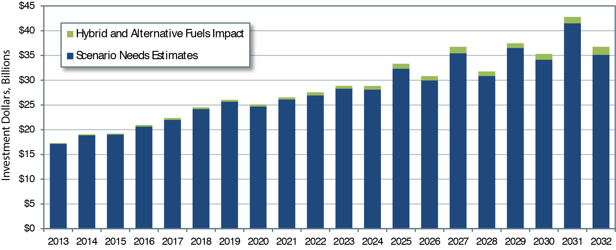
Exhibit 9-5 indicates how alternative assumptions regarding the timing of investment would impact the distribution of spending among the four 5-year funding periods considered in HERS, and how these spending patterns could affect pavement condition (measured using the International Roughness Index [IRI]) and average delay per VMT. The investment levels were selected from the baseline HERS analyses for Federal-aid highways presented in Chapter 7 to compare across the three investment patterns: baseline ramped spending, flat spending, and BCR-driven spending. The average annual investment requirement is kept constant in all three cases to compare the impact of different investment patterns, even when the total amount of spending is identical. The average annual investment requirement is set at $75.4 billion, which is the HERS-derived input to the Improve Conditions and Performance scenario in Chapter 8.
Exhibit 9-5 Impact of Investment Timing on HERS Results Reflected in the Improve Conditions and Performance Scenario-Effects on Pavement Roughness and Delay per VMT
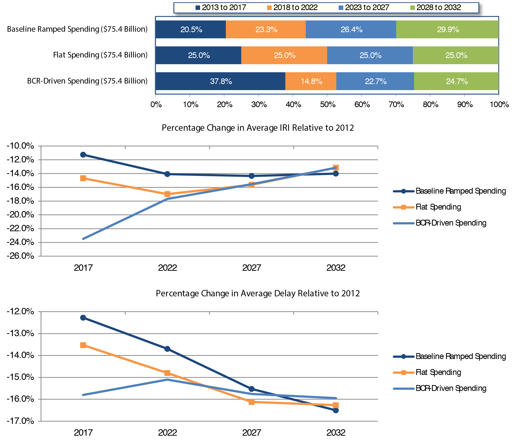
Source: Highway Economic Requirements System.
As shown in the top panel of Exhibit 9-5, the level of investment grows over time in the baseline ramped spending case assuming a constant growth of real investment. Under this scenario, annual investment would grow by 2.53 percent per year from $57.4 billion in 2013 to $94.6 billion in 2032, which totals $1,508 billion over 20 years or $75.4 billion per year in constant 2012 dollars. Only 20.5 percent of the total 20-year investment occurs in the first 5-year period, 2013 to 2017, while 29.9 percent of total investment occurs in the last 5-year period, 2028 to 2032. Under the flat spending alternative, investment is equally distributed over time so that each 5-year period accounts for exactly one-quarter of the total 20-year investment.
The HERS-modeled and BCR-driven spending alternative displays a different investment pattern. A high proportion of total spending, 37.8 percent of total investment, would occur in the first 5year period to address the large backlog of cost-beneficial investment the system is facing now (see Backlog discussion in Chapter 8). Under this alternative, investment needs in the second 5year period would drop to 14.8 percent of the total 20-year need. Investment needs would increase in the last two 5-year periods because many roadways that were rehabilitated in the first 5-year period would need to be resurfaced or reconstructed again.
Impacts of Alternative Investment Patterns
An obvious difference among the three alternative investment patterns is that the higher the level of investment within the first 5-year analysis period, the better the level of performance achieved by 2017.
The middle panel of Exhibit 9-5 presents percentage changes of average pavement roughness as measured by IRI compared with the 2012 level under the three investment cases. A reduction in average IRI represents improvement in pavement conditions. The graph shows that the BCR-driven spending case yields the greatest improvement in pavement conditions in the first 5-year period, represented by a large drop in average IRI by more than 20 percent from its 2012 level. The improvement under the BCR-driven spending alternative shrinks to about 13 percent by the last 5-year period. Steady pavement improvement over time is achieved in baseline ramped spending and flat spending assumptions. In the first 5 years, average IRI decreases by approximately 15 percent (relative to the 2012 level) under the flat spending case and the descending trend continues across the rest of the analysis periods. The baseline ramped spending assumption leads to an 11-percent drop in average IRI in the first 5-year period and further improvement in pavement afterward, but the improvement is not as pronounced as for the flat spending alternative. The decreases of average IRI are similar by 2032 under all three cases.
The bottom panel of Exhibit 9-5 illustrates the progress in average delay reduction across three investment cases. The percentage change of average delay, relative to its 2012 level, remains negative, indicating a decrease in average delay of travelers. In the first 5 years, the BCR-driven spending approach results in the largest reduction in average delay per VMT, 16 percent , and the baseline ramped spending the smallest reduction, 12 percent . The percentages of delay reduction grow over time under the baseline ramped and flat spending cases, suggesting sustained benefits through capital investment to improve pavement. The percentage change of average delay is stable under BCR-driven spending. By the end of the 20-year analysis period, the difference between projected average delay and the 2012 delay will be approximately 16 percent under all three alternatives.
These results show that the BCR-driven approach achieves the highest IRI and delay reduction in the medium run (the first 5-year period). The baseline ramped spending approach results in the smallest pavement and delay improvement over the same period. System performance, however, does not differ substantially across investment timing in the long run of 20 years. Based on this analysis, the key advantage to front-loading highway investment is not in reducing 20-year total investment needs; instead, the strength of BCR-driven spending lies in the years of additional benefits that highway users would accrue over time if system conditions and performance were improved earlier in the 20-year analysis period.
Alternative Timing of Investment in NBIAS
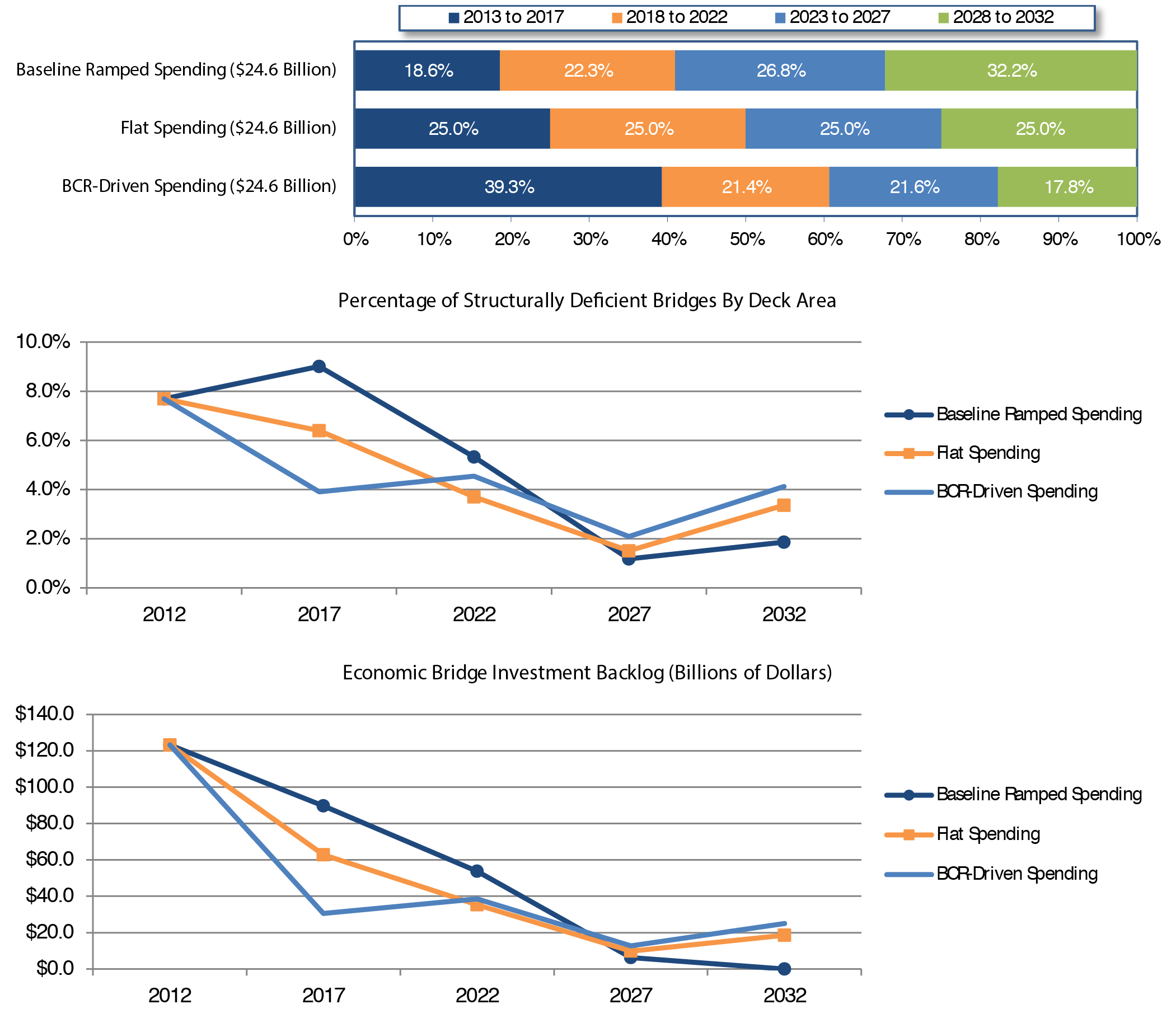
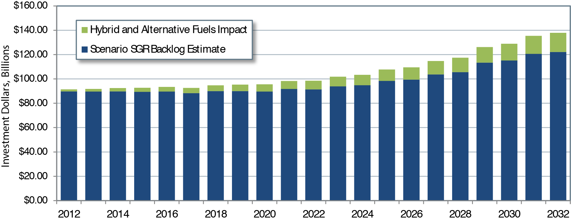
Exhibit 9-6 identifies the impacts of alternative investment timing on the share of bridges that are structurally deficient by deck area using the three investment assumptions described above: baseline ramped spending, flat spending, and BCR-driven spending. The average annual investment level of each alternative analyzed ($24.6 billion) corresponds to NBIAS-derived input to the Improve Conditions and Performance scenario presented in Chapter 8.
Similar to the results of pavement investment in HERS presented earlier, investment timing has an impact on structurally deficient bridges. The baseline ramped case for the NBIAS Improve Conditions and Performance scenario assumes constant annual spending growth of 3.72 percent from its 2012 level, with a total 20-year investment of $492.1 billion and an average annual investment of $24.6 billion in constant 2012 dollars. The top panel of Exhibit 9-6 indicates that more investment occurs in the later years under the baseline ramped case of gradual and constant growth-about 32.2 percent in the last 5-year period. The BCR-driven spending case requires a large portion of the total 20-year investment in the first 5-year period (39.3 percent ), then declines to 17.8 percent in the last 5-year period. Spending levels remain constant in the flat spending case.
A different investment pattern produces substantially different outcomes. The middle panel of Exhibit 9-6 shows that the greatest bridge improvement in the first 5-year period occurs under the BCR-driven spending assumption, as the share of structurally deficient bridges by deck area drops from 7.7 percent in 2012 to 3.9 percent in 2017. During the same period, the share of structurally deficient bridges decreases to 6.4 percent under the flat spending assumption but increases to 9 percent under the baseline ramped spending assumption. In the next 15 years, however, this pattern is reversed. At an average annual investment level of $24.6 billion, NBIAS projects that the lowest share of structurally deficient bridges in 2032 would be achieved under the baseline ramped spending approach with 1.9 percent of bridges that are structurally deficient, compared to 3.4 percent assuming flat spending and 4.1 percent for the BCR-driven spending alternative.
The economic bridge investment backlog also exhibits different trends under the alternative investment timing. The lower panel of Exhibit 9-6 indicates that, from 2012 to 2017, the average backlog declines sharply under the BCR-driven alternative, with slower declines under the flat spending alternative and baseline ramped spending. The rate of decline is determined by the investment timing. High bridge investment in later years under baseline ramped spending leads to the elimination of economic backlog by 2032, while the projected backlog will be $18.5 billion and $25 billion under the flat spending and BCR-driven spending assumptions, respectively.
Exhibit 9-6 Impact of Investment Timing on NBIAS Results Reflected in the Improve Conditions and Performance Scenario-Effects on Structurally Deficient Bridges and Economic Bridge Investment Backlog
Source: National Bridge Investment Analysis System.
The indicators suggest that continued baseline ramped spending for bridges would yield the best outcomes by 2032. The share of structurally deficient bridges and investment backlog start to increase in the last 5-year period under the flat spending and BCR-driven spending assumptions, however, highlighting a potential surge of investment needs by the end of the analysis period under these spending assumptions.
Accounting for Inflation
The analysis of potential future investment/performance relationships in the C&P report has traditionally stated future investment levels in constant dollars, with the base year set according to the year of the conditions and performance data supporting the analysis. Throughout Chapters 7 and 8, this edition of the C&P report has stated all investment levels in constant 2012 dollars. For some purposes, however, such as comparing investment spending in a particular scenario with nominal dollar revenue projections, adjusting for inflation to present spending in nominal dollar terms might be desirable. Given an assumption about future inflation, the C&P report's constant-dollar numbers could be converted to nominal dollars or the nominal projected revenues could be converted to constant 2012 dollars for comparison purposes. Exhibit 9-7 takes the former approach by converting constant-dollar values to nominal dollars.
The average annual increase in highway construction costs over the past 20 years (1992 to 2012) was 2.9 percent . Since the creation of the Federal Highway Trust Fund in 1956, the 20-year period with the smallest increase in construction costs was 1980 to 2000, when costs grew by 2.0 percent per year. (Historic inflation rates were determined using the FHWA Composite Bid Price Index through 2006, and the new FHWA National Highway Construction Cost Index from 2006 to 2012; these indices are discussed in Chapter 6.) Exhibit 9-7 illustrates how the constant-dollar figures associated with three scenarios for highways and bridges presented in Chapter 8 could be converted to nominal dollars based on two alternative annual inflation rates of 2.0 percent (historically lowest rate) and 2.9 percent (past 20 years' rate).
The systemwide Sustain 2012 Spending scenario presented in Chapter 8 assumes that combined capital spending for highway and bridge improvements would be sustained at its 2012 level in constant-dollar terms for 20 years. Thus, the first column in Exhibit 9-7 shows $105.2 billion of spending in constant 2012 dollars for each year from 2013 to 2032, for a 20-year total of $2.1 trillion. Applying annual inflation in construction costs at 2.0 percent or 2.9 percent would imply a 20-year total in nominal dollars of $2.6 trillion or $2.9 trillion, respectively.
Exhibit 9-7 Illustration of Potential Impact of Alternative Inflation Rates on Selected Systemwide Investment Scenarios |
|||||||||
|---|---|---|---|---|---|---|---|---|---|
| Year | Highway Capital Investment (Billions of Dollars) | ||||||||
| Constant 2012 Dollars1 | Nominal Dollars (Assuming 2.0 percent Annual Inflation) | Nominal Dollars (Assuming 2.9 percent Annual Inflation) | |||||||
| Sustain 2012 Spending Scenario | Maintain Conditions & Performance Scenario | Improve Conditions & Performance Scenario | Sustain 2012 Spending Scenario | Maintain Conditions & Performance Scenario | Improve Conditions & Performance Scenario | Sustain 2012 Spending Scenario | Maintain Conditions & Performance Scenario | Improve Conditions & Performance Scenario | |
| 2012 | $105.2 | $105.2 | $105.2 | $105.2 | $105.2 | $105.2 | $105.2 | $105.2 | $105.2 |
| 2013 | $105.2 | $103.6 | $108.2 | $107.3 | $105.7 | $110.3 | $108.2 | $106.6 | $111.3 |
| 2014 | $105.2 | $102.0 | $111.2 | $109.4 | $106.1 | $115.7 | $111.4 | $108.0 | $117.7 |
| 2015 | $105.2 | $100.5 | $114.3 | $111.6 | $106.6 | $121.3 | $114.6 | $109.5 | $124.6 |
| 2016 | $105.2 | $98.9 | $117.5 | $113.9 | $107.1 | $127.2 | $117.9 | $110.9 | $131.8 |
| 2017 | $105.2 | $97.4 | $120.8 | $116.1 | $107.6 | $133.4 | $121.4 | $112.4 | $139.4 |
| 2018 | $105.2 | $95.9 | $124.2 | $118.5 | $108.0 | $139.9 | $124.9 | $113.9 | $147.5 |
| 2019 | $105.2 | $94.5 | $127.7 | $120.8 | $108.5 | $146.7 | $128.5 | $115.4 | $156.0 |
| 2020 | $105.2 | $93.0 | $131.3 | $123.3 | $109.0 | $153.9 | $132.2 | $116.9 | $165.1 |
| 2021 | $105.2 | $91.6 | $135.0 | $125.7 | $109.5 | $161.3 | $136.1 | $118.5 | $174.6 |
| 2022 | $105.2 | $90.2 | $138.8 | $128.2 | $110.0 | $169.2 | $140.0 | $120.1 | $184.7 |
| 2023 | $105.2 | $88.8 | $142.7 | $130.8 | $110.5 | $177.4 | $144.1 | $121.7 | $195.4 |
| 2024 | $105.2 | $87.5 | $146.7 | $133.4 | $111.0 | $186.1 | $148.3 | $123.3 | $206.8 |
| 2025 | $105.2 | $86.2 | $150.8 | $136.1 | $111.4 | $195.1 | $152.5 | $124.9 | $218.7 |
| 2026 | $105.2 | $84.8 | $155.1 | $138.8 | $111.9 | $204.6 | $157.0 | $126.6 | $231.4 |
| 2027 | $105.2 | $83.5 | $159.4 | $141.6 | $112.4 | $214.6 | $161.5 | $128.3 | $244.8 |
| 2028 | $105.2 | $82.3 | $163.9 | $144.4 | $112.9 | $225.0 | $166.2 | $130.0 | $259.0 |
| 2029 | $105.2 | $81.0 | $168.5 | $147.3 | $113.4 | $236.0 | $171.0 | $131.7 | $274.0 |
| 2030 | $105.2 | $79.8 | $173.3 | $150.2 | $113.9 | $247.5 | $176.0 | $133.5 | $289.9 |
| 2031 | $105.2 | $78.6 | $178.1 | $153.3 | $114.5 | $259.5 | $181.1 | $135.2 | $306.6 |
| 2032 | $105.2 | $77.4 | $183.1 | $156.3 | $115.0 | $272.1 | $186.3 | $137.0 | $324.4 |
| Total | $2,104.0 | $1,797.5 | $2,850.9 | $2,607.2 | $2,205.0 | $3,597.0 | $2,879.3 | $2,424.3 | $4,003.7 |
| 0.00% | -1.52% | 2.81% | Constant-Dollar Growth Rate | ||||||
| $105.2 | $89.9 | $142.5 | Average Annual Investment Level in Constant 2012 Dollars | ||||||
1 Based on average annual investment levels and annual constant-dollar growth rates identified in Exhibit 8-2. Source: FHWA staff analysis. | |||||||||
Chapter 8 indicates that achieving the objectives of the systemwide Maintain Conditions and Performance scenario would require investment averaging $89.9 billion per year in constant 2012 dollars. The investment totals $1.8 billion over 20 years (2013 to 2032) in constant-dollar spending, equivalent to spending that steadily decreases at 1.52 percent per year. Exhibit 9-7 illustrates the application of this real reduction rate, demonstrating how annual capital investment in constant-dollar terms would decrease from $105.2 billion in 2012 to $77.4 billion in 2032. A 2.0-percent inflation rate applied to these constant-dollar estimates would produce a 20-year total cost of $2.2 trillion in nominal dollars, while a 2.9-percent inflation rate results in a total cost of $2.4 trillion.
The investment/performance models discussed in this report estimate the future benefits and costs of transportation investments in constant-dollar terms. This practice is standard for this type of economic analysis. Converting the model outputs from constant dollars to nominal dollars is necessary to adjust them to account for projected future inflation.
Traditionally, this type of adjustment has not been made in the C&P report. Because inflation prediction is an inexact science, adjusting the constant-dollar figures to nominal dollars tends to add to the uncertainty of the overall results and make the report more difficult to use if the inflation assumptions are inaccurate. Allowing readers to make their own inflation adjustments based on actual trends observed after publication of the C&P report or based on the most recent projections from other sources is expected to yield a better overall result, particularly given the sharp swings in recent years in material costs for highway construction.
The use of constant-dollar figures also is intended to provide readers with a reasonable frame of reference in terms of an overall cost level that they have recently experienced. When inflation rates are compounded for 20 years, even relatively small growth rates can produce nominal dollar values that appear very large when viewed from the perspective of today's typical costs.
The compounding impacts of inflation are even more evident for the systemwide Improve Conditions and Performance scenario. As described in Chapter 8, this scenario assumes 2.81percent growth in constant-dollar highway capital spending per year to address all potentially cost-beneficial highway and bridge improvements by 2032. The 20-year total investment level of $2.9 trillion associated with this scenario equates to an average annual investment level of $142.5 billion in constant 2012 dollars. Adjusting this figure to account for inflation of 2.0 percent or 2.9 percent would result in 20-year total nominal dollar costs of $3.6 trillion or $4.0 trillion, respectively.
Transit Supplemental Scenario Analysis
This section provides a more detailed discussion of the assumptions underlying the scenarios presented in Chapters 7 and 8 and of the real-world issues that affect transit operators' ability to address their outstanding capital needs. Specifically, this section discusses the following topics:
- asset condition forecasts under three scenarios: (1) Sustain 2012 Spending, (2) Low-Growth, and (3) High-Growth; in addition, the analysis includes a discussion of the State of Good Repair Benchmark;
- a comparison of recent historic passenger miles traveled (PMT) growth rates with the revised low-growth and high-growth projections;
- an assessment of the impact on the backlog estimate of purchasing hybrid vehicles; and
- the forecast of purchased transit vehicles, route miles, and stations under the Low- and High-Growth scenarios.
Asset Condition Forecasts and Expected Useful Service Life Consumed for All Transit Assets under Three Scenarios and the SGR Benchmark
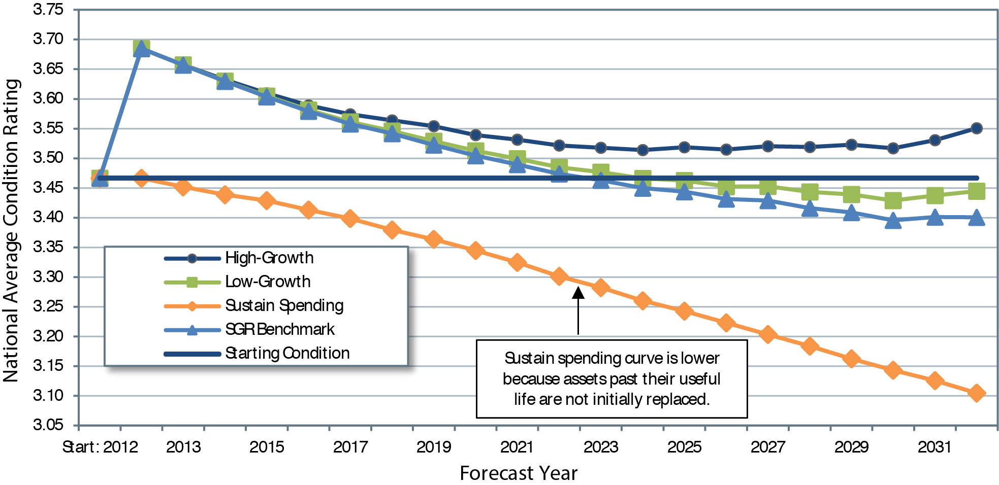
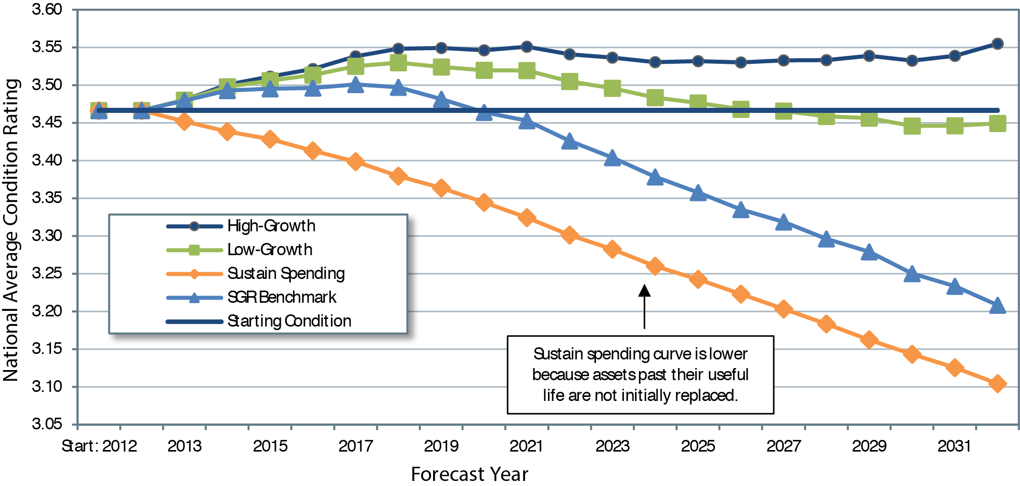
As in the 2013 edition, this edition of the C&P report uses three condition projection scenarios (i.e., Sustain 2012 Spending, Low-Growth, and High-Growth scenarios) and the State of Good Repair (SGR) Benchmark to understand better which condition outcome is desirable or even sensible. For example, are current asset conditions at an acceptable level or are they too low (or too high) for individual asset types?
To help answer this question, Exhibit 9-8 presents the condition projections for each of the three scenarios and the SGR Benchmark. Note that these projections predict the condition of all transit assets in service during each year of the 20-year analysis period, including transit assets that exist today and any investments in expansion assets by these scenarios. The Sustain 2012 Spending, Low-Growth, and High-Growth scenarios each make investments in expansion assets while the SGR Benchmark reinvests only in existing assets. Note that the estimated current average condition of the Nation's transit assets is 3.45. As discussed in Chapter 8, expenditures under the financially constrained Sustain 2012 Spending scenario are not sufficient to address replacement needs as they arise, leading to a predicted increase in the investment backlog. This increasing backlog is a key driver in the decline in average condition of transit assets, as shown for this scenario in Exhibit 9-8.
Exhibit 9-8 Asset Condition Forecast for All Existing and Expansion Transit Assets
Source: Transit Economic Requirements Model.
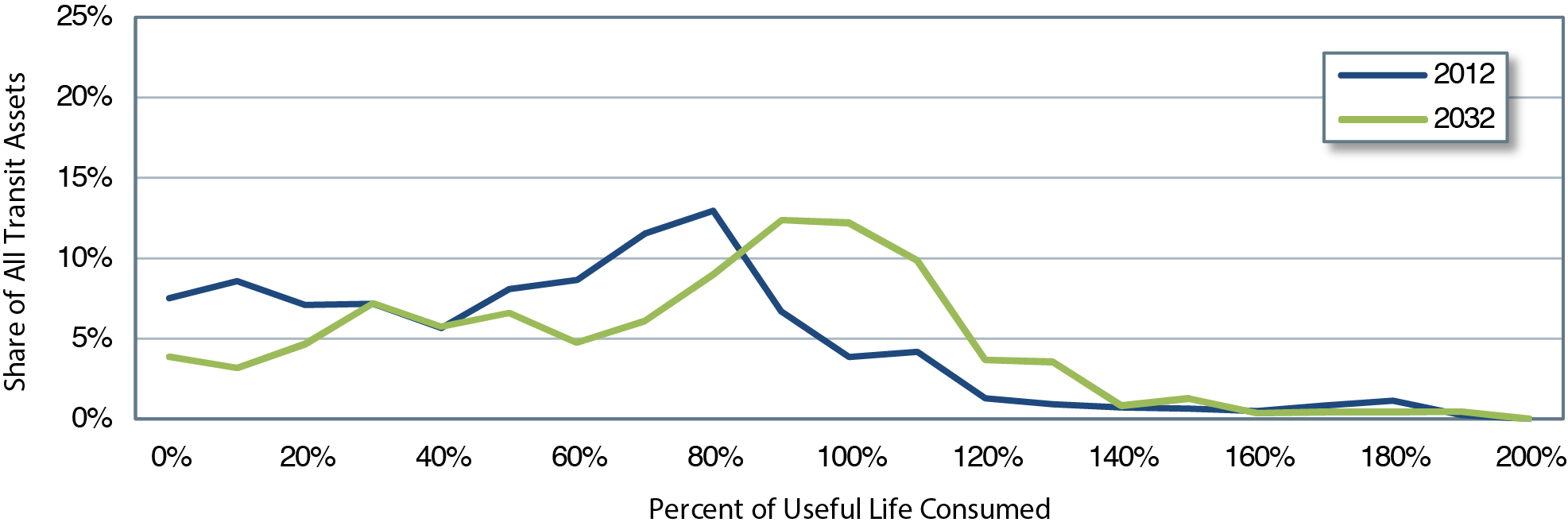
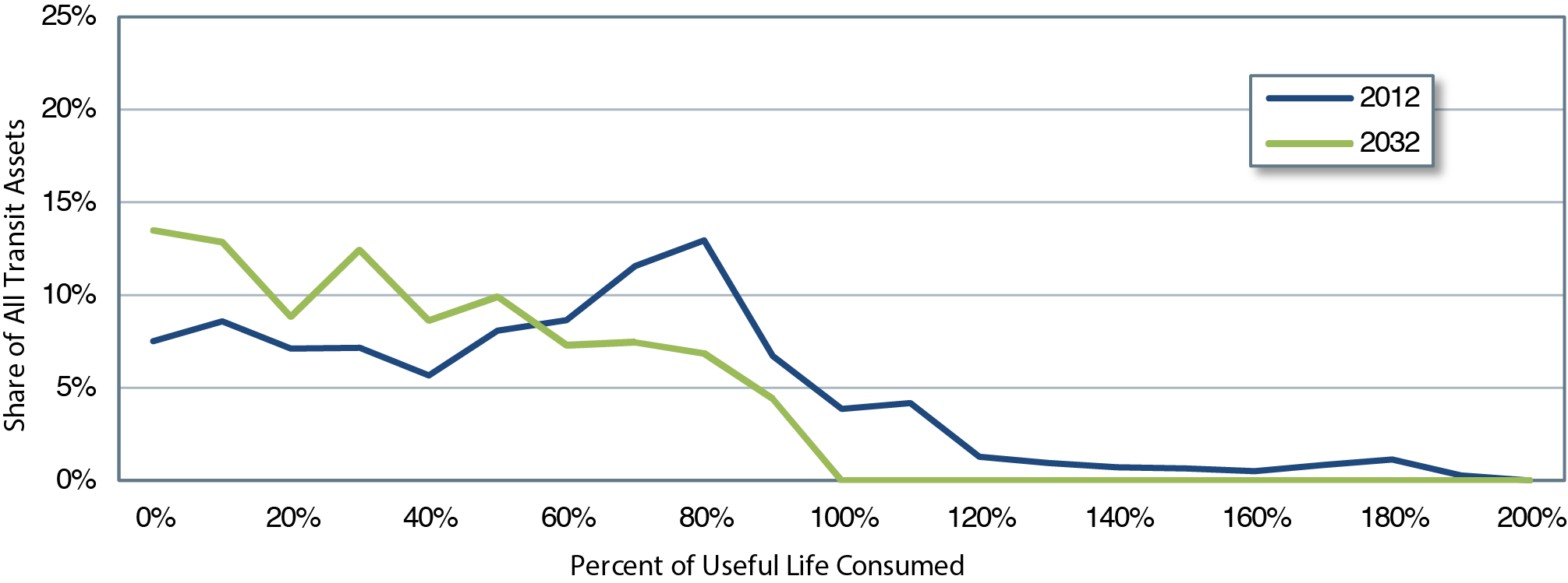
If the SGR Benchmark represents a reasonable long-term investment strategy (i.e., replacing assets close to the end of their useful life, which results in a long-term decline in average conditions), investing under the Sustain 2012 Spending scenario implies an investment strategy of replacing assets at later ages, in worse conditions, and potentially after the end of their useful life, as shown in Exhibit 9-9. Expenditures on asset reinvestment for the Sustain 2012 Spending scenario are insufficient to address ongoing reinvestment needs, leading to an increase in the size of the backlog. Note that the forecast for 2032 for the Sustain 2012 Spending scenario shown in Exhibit 9-9 indicates that assets under this scenario will be closer to or beyond the end of their useful lives, when compared with the other scenarios; this difference reflects a larger portion of the national transit assets still in use after the end of their useful lives.
Exhibit 9-9 Sustain 2012 Spending Scenario: Asset percent of Useful Life Consumed
Source: Transit Economic Requirements Model.
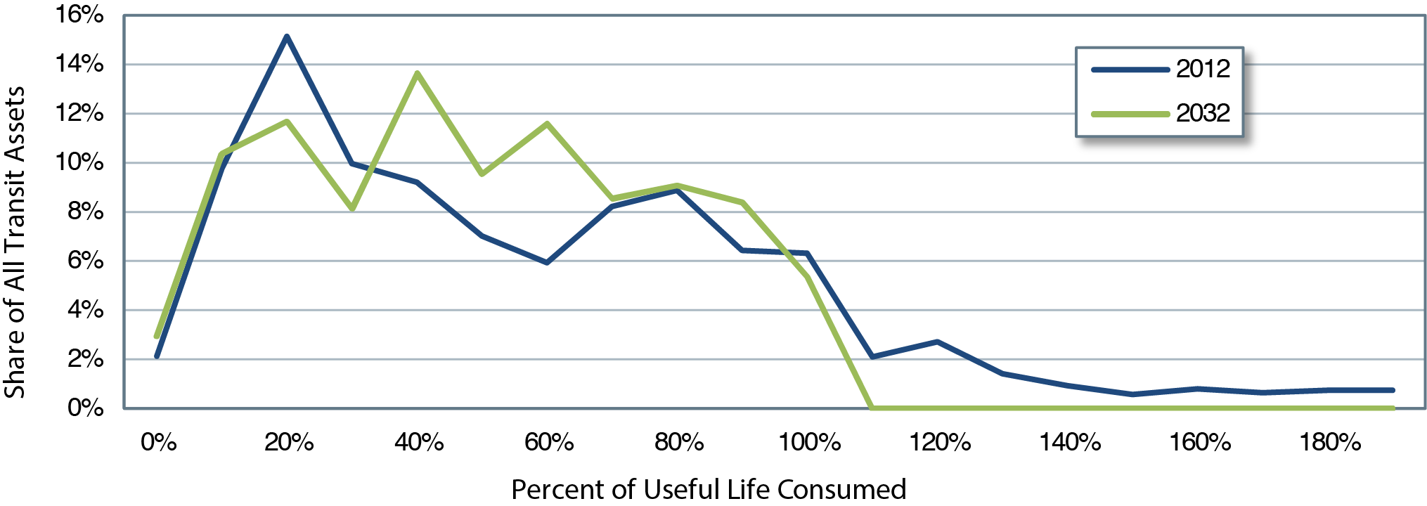
In contrast to the Sustain 2012 Spending scenario, the SGR Benchmark is financially (and economically)_unconstrained and considers the level of investment required to both eliminate the current investment backlog and to address all ongoing reinvestment needs as they arise such that all assets remain in an SGR (i.e., a condition of 2.5 or higher). Despite adopting the objective of maintaining all assets in an SGR throughout the forecast period, average conditions under the SGR Benchmark ultimately decline to levels below the current average condition value of 3.45.
This result, although counterintuitive, is explained by a high proportion of long-lived assets (e.g., guideway structures, facilities, and stations) that currently have high average condition ratings and a significant amount of useful life remaining, as shown in Exhibit 9-10. The exhibit shows the share of all transit assets (equal to approximately $804 billion in 2012) as a function of useful life consumed. Eliminating the current SGR backlog removes a significant number of over-age assets from service (resulting in an initial jump in asset conditions). The ongoing aging of the longer-lived assets, however, ultimately will draw the average asset conditions down to a long-term condition level that is consistent with the objective of SGR (and hence sustainable) but ultimately measurably below current average aggregate conditions.
Exhibit 9-10 SGR Benchmark: Asset percent of Useful Life Consumed
Source: Transit Economic Requirements Model.
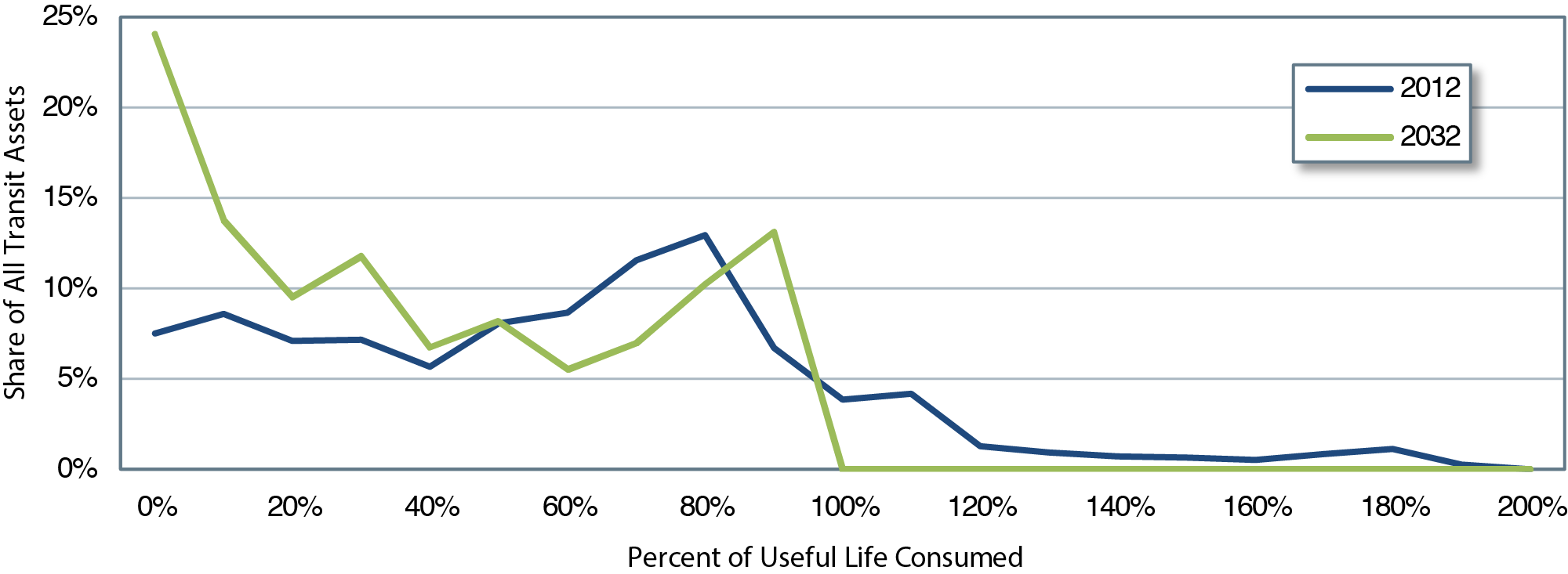
To underscore these findings, note that the Low- and High-Growth scenarios include unconstrained investments in both asset replacements and asset expansions. Hence, not only are older assets replaced as needed with an aggressive reinvestment rate, but also new expansion assets are also continually added to support ongoing growth in travel demand. Although initially insufficient to arrest the decline in average conditions completely, the impact of these expansion investments ultimately would reverse the downward decline in average asset conditions in the final years of the 20-year projections. A higher proportion of long-lived assets with more useful life remaining in 2032 than in 2012 also would result, as illustrated in Exhibit 911 and Exhibit 912, respectively. Furthermore, the High-Growth scenario (Exhibit 9-12) adds newer expansion assets at a higher rate than does the Low-Growth scenario (Exhibit 9-11), ultimately yielding higher average condition values for that scenario (and average condition values that exceed the current average of 3.45 throughout the entire forecast period).
Exhibit 9-11 Low-Growth Scenario: Asset percent of Useful Life Consumed
Source: Transit Economic Requirements Model.
Exhibit 9-12 High-Growth Scenario: Asset percent of Useful Life Consumed
Source: Transit Economic Requirements Model.
Alternative Methodology
When current transit investment practices are considered, the level of investment needed to eliminate the SGR backlog in 1 year is infeasible. Thus, the SGR Benchmark, Low-Growth, and High-Growth scenarios' financially unconstrained assumptions (e.g., spending of unlimited transit investment funds each year) are unrealistic. As indicated in Exhibit 9-8, the elimination of the backlog in the first year and the resulting jump in asset conditions in year 1 can be attributed to this unconstrained assumption.
An alternative, more-feasible methodology is to have the Low- and High-Growth scenarios, and the SGR Benchmark, use a financially constrained reinvestment rate to eliminate the SGR backlog by year 20 while maintaining the collective national transit assets at a condition rating of 2.5 or higher. Analysis has determined that investing $16.6 billion annually would eliminate the backlog in 20 years.
Exhibit 9-13 presents the condition projections for the two scenarios and the benchmark using this alternative methodology. The Low- and High-Growth scenarios and SGR Benchmark are financially constrained so the investment strategies result in replacing assets at later ages, in worse conditions, and potentially after the end of their useful lives.
Exhibit 9-13 Asset Condition Forecast for All Existing and Expansion Transit Assets
Source: Transit Economic Requirements Model.
Revised Method for Estimating PMT Growth Rates
The Low-and High-Growth scenarios presented in Chapters 7 and 8 estimate the level of investment in expansion assets (e.g., additional passenger vehicles, maintenance facilities, stations, and miles of track) required to support growth in ridership over the upcoming 20-year period. Specifically, these scenarios are designed to expand investment in passenger vehicles and related assets at the same rate of growth as the projected rate of increase in PMT, ensuring that the ratio of riders to transit assets (e.g., riders per vehicle) remains at today's levels throughout the entire forecast period. [1] Here, the Low-Growth scenario provides the level of expansion investment as required to support relatively low PMT growth (lower bound). In contrast, the High-Growth scenario supports an upper-bound estimate of future PMT growth. The actual rate of increase in PMT and related expansion needs are expected to fall somewhere between these bounds.
Change in Methodology: For this report, FTA has applied a new methodology for estimating PMT growth for use in the Low- and High-Growth scenarios. This revised approach is believed to be more accurate and it provides greater consistency between the Low- and High-Growth scenarios compared with the prior approach. Following is an explanation of the methodology used to estimate growth in PMT in previous C&P reports and the new methodology used for this report.
Prior Methodology: Prior to this report, the Low- and High-Growth scenarios used different (and hence inconsistent) approaches to project the rate of increase in PMT (Exhibit 9-14). Note that in previous years, PMT growth was modeled at the urbanized area (UZA) level (i.e., the same growth rate would be applied to all agencies and modes within a given UZA).
Low-Growth: For prior-year C&P reports, PMT growth rates for the Low-Growth scenario were obtained from a sample of the Nation's metropolitan planning organizations (MPOs). Specifically, this sample included the MPOs representing all of the Nation's 30 largest UZAs and a sample of 30 or more MPOs from small and mid-sized UZAs. MPOs prepare ridership and PMT projections using detailed ridership models and use the results for urban planning purposes. Note that MPO ridership forecasts are financially constrained and, for this reason, the MPO projections were used for the Low-Growth scenario.
High-Growth: For prior-year C&P reports, PMT growth for the High-Growth scenario was based on the weighted average trend rate of growth for each UZA. These UZA-specific weighted-average growth rates were calculated across all agencies and modes within a given UZA, using the most recent 15 years of historical National Transit Database data. Hence, under this approach, all agencies and modes within a UZA were projected to have the same trend rate of PMT growth.
Revised Methodology (2015 C&P Report): For this report, the PMT growth rates used in the Low- and High-Growth scenarios are calculated using a common approach (Exhibit 9-14). Specifically, both scenarios are based on the trend rate of PMT growth for all riders using the same mode, within UZAs of similar size (large, medium, or small) and within the same FTA region. This approach also used 15 years of data from the National Transit Database to establish a trend rate of increase. Finally, the Low-Growth scenario used the trend rate of increase minus 0.5 percent while the High-Growth scenario used the trend rate of increase plus 0.5 percent .
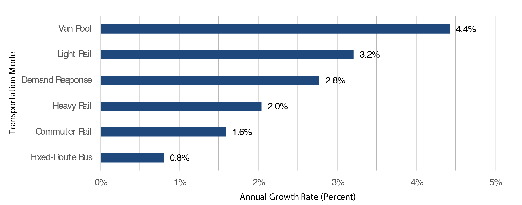
Impact of Change: A key benefit of this revised approach is the recognition that the PMT growth rates can be and have been significantly different by mode (Exhibit 9-15). For example, over the most recent 15-year period, PMT for motor bus has tended to be flat while the rate of increase for heavy rail, demand response, and vanpool has been high. The result is decreased bus expansion needs and increased needs for heavy rail and demand-response expansion as compared to prior-year reports. In addition, the revised approach also recognizes that growth rates can differ significantly by urban area size and geographic region.
Exhibit 9-15 Passenger Miles Traveled: 15-Year Compound Annual Growth Rate by Mode,1997-20121
1Adjusted to remove outliers.
Source: Transit Economic Requirements Model.
Impact of New Technologies on Transit Investment Needs
The investment needs scenarios presented in Chapter 8 implicitly assume that all replacement and expansion assets will use the same technologies as are currently in use today (i.e., all asset replacement and expansion investments are "in kind"). As with most other industries, however, the existing stock of assets used to support transit service is subject to ongoing technological change and improvement, and this change tends to result in increased investment costs (including future replacement needs). Although many improvements are standardized and hence embedded in the asset (i.e., the transit operator has little or no control over this change), numerous instances occur where transit operators have intentionally selected technology options that are significantly more costly than preexisting assets of the same type. A key example is the frequent decision to replace diesel motor buses with compressed natural gas or hybrid buses. Although such options offer clear environmental benefits (and compressed natural gas might decrease operating costs), acquisition costs for these vehicle types are 20 to 60 percent higher than diesel. This increase in cost generally increases current and long-term reinvestment needs and, in a budget-constrained environment, increases the expected future size of the investment backlog. This increase might be offset by lower operating costs from more reliable operation, longer useful lives, and improved fuel efficiency, but this possible offset is not captured in this assessment of capital needs. Again, the effect of technology-driven increases in needs is not included in the needs estimates presented in Chapters 7 and 8 of this report.
In addition to improvements in preexisting asset types, transit operators periodically expand their existing asset stock to introduce new asset types that take advantage of technological innovations. Examples include investments in intelligent transportation system technologies such as real-time passenger information systems and automated dispatch systems-assets and technologies that are common today but were not available 15 to 20 years ago. These improvements typically yield improvements in service quality and efficiency, but they also tend to yield increases in asset acquisition, maintenance, and replacement costs, resulting in an overall increase in reinvestment costs and the expected future size of the SGR backlog.
Impact of Compressed Natural Gas and Hybrid Buses on Future Needs
To provide a better sense of the impact of new technology adoption on long-term needs, the analysis below presents estimates of the long-term cost of the shift from diesel to compressed natural gas and hybrid buses. Important to emphasize is that this analysis is intended to provide only a sense of the significance of this impact on long-term capital needs (including the possible consequences of not capturing this impact in TERM's needs estimates). This assessment is not one of the full range of operational, environmental, or other potential costs and benefits arising from this shift and, hence, it does not evaluate the decision to invest in any specific technology.
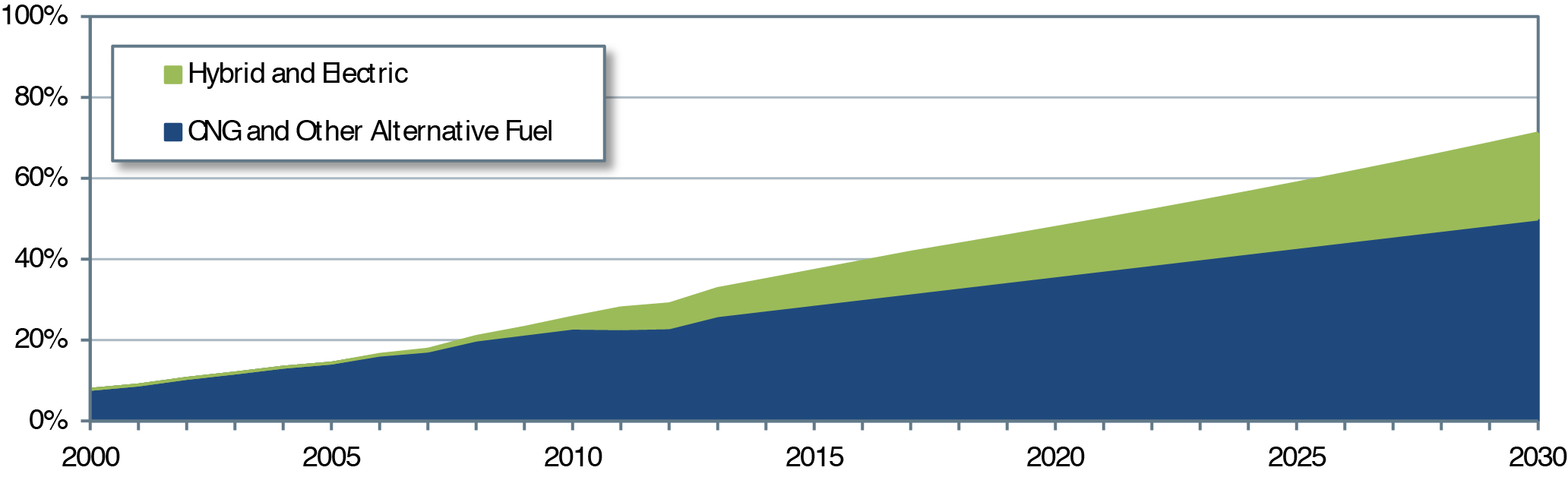
Exhibit 9-16 presents historical (2000—2012) and forecast (2013—2030) estimates of the share of transit buses that rely on compressed natural gas and other alternative-fuel vehicles and on hybrid power sources. The forecast estimates assume the current trend rate of increase in alternative and hybrid vehicle shares as observed from 2007 to 2012. Based on this projection, the share of vehicles powered by alternative fuels is estimated to increase from 26 percent in 2012 to 50 percent in 2030. During the same period, the share of hybrid buses is estimated to increase from 6 percent to 21 percent . This results in diesel shares declining from roughly 71 percent today to about 29 percent by 2030.
Exhibit 9-16 Hybrid and Alternative Fuel Vehicles: Share of Total Bus Fleet, 2000—2030
Source: Transit Economic Requirements Model.
Impact on Costs
According to a 2007 report by FTA, Transit Bus Life Cycle Cost and Year 2007 Emissions Estimation, the average unit cost of an alternative-fuel bus plus its share of cost for the required fueling station is 15.5 percent higher than that of a standard diesel bus of the same size. Similarly, hybrid buses cost roughly 65.9 percent more than standard diesel buses of the same size. When combined with the current and projected mix of bus vehicle types presented above in Exhibit 9-16, these cost assumptions yield an estimated increase in average capital costs for bus vehicles of 14.3 percent from 2012 to 2030 (using the mix of bus types from 2012 as the base of comparison). (Note that this cost increase represents a shift in the mix of bus types purchased and not the impact of underlying inflation, which will affect all vehicle types, including diesel, alternative fuels, and hybrid.) Reductions in operating costs due to the new technology are not shown in this analysis of capital needs but are presumably part of the motivation for agencies that purchase these vehicles.
Impact on Needs
What, then, is the impact of this cost increase on long-term transit capital needs? Exhibit 9-17 presents the impact of this potential cost increase on annual transit needs as estimated for the Low-Growth scenario presented in Chapter 8. For this scenario, the cost impact is negligible in the early years of the projection period but grows over time as the proportion of buses using alternative fuel and hybrid power increases (note that the investment backlog is not included in this depiction). The impact on total investment needs for Chapter 9 investment scenarios (Low-Growth and High-Growth) and the SGR Benchmark are presented in dollar and percentage terms in Exhibit 9-18. Note that the shift to alternative fuels and hybrid buses is estimated to increase average annual replacement needs by $0.5 billion to $0.8 billion, yielding a 2.5- to 3.5-percent increase in investment needs. To provide perspective for these estimated amounts, noting the following is helpful: (1) the shift from diesel to alternative-fuel and hybrid buses is only one of several technology changes that might affect long-term transit reinvestment needs, but (2) reinvestment in transit buses likely represents the largest share of transit needs subject to this type of significant technological change. Hence, the impact of all new technology adoptions (not accounted for in the Chapter 8 scenarios and including new bus propulsion systems) might add 5—10 percent to long-term transit capital needs.
Exhibit 9-17 Impact of Shift to Vehicles Using Hybrid and Alternative Fuels on Investment Needs:Low-Growth Scenario
Source: Transit Economic Requirements Model.
Impact on Backlog
Finally, in addition to affecting unconstrained capital needs, the shift from diesel to hybrid and alternative-fuel vehicles also can affect the size of the future backlog. For example, Exhibit 919 shows the estimated impact of this shift on the SGR backlog as estimated for the Sustain 2012 Spending scenario from Chapter 8. Under this scenario, long-term spending is capped at current levels such that any increase in costs over the analysis period must necessarily be added to the backlog. Moreover, given that the useful lives of buses as estimated by TERM are roughly 7—14 years, all existing and many expansion vehicles will need to be replaced over the 20-year analysis period, meaning that any increase in costs for this asset type will be added to the backlog for the period of analysis.
Exhibit 9-19 Impact of Shift to Vehicles Using Hybrid and Alternative Fuels on Backlog Estimate:Sustain 2012 Spending Scenario
Source: Transit Economic Requirements Model.
As with the analysis above, Exhibit 9-19 suggests that the initial impact of the shift to hybrid and alternative-fuel vehicles is small but the effect increases over time as the share of the Nation's bus fleet made up by these vehicle types increases. By 2030, this shift is estimated to increase the size of the backlog from $141.7 billion to $151.4 billion, an increase of $9.8 billion or 6.9 percent .
Forecasted Expansion Investment
This section compares key characteristics of the national transit system in 2012 to their forecasted TERM results over the next 20 years for different scenarios. It also includes expansion projections of fleet size, guideway route miles, and stations broken down by scenario to understand better the expansion investments that TERM forecasts.
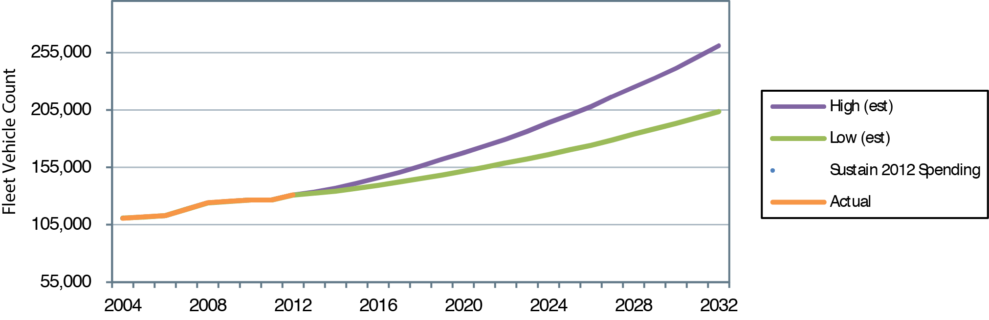
TERM's projections of fleet size are presented in Exhibit 9-20. The projections for the Low- and High-Growth scenarios create upper and lower bounds around the projected Sustain 2012 Spending scenario to preserve existing transit assets at a condition rating of 2.5 or higher and expand transit service capacity to support differing levels of ridership growth while passing TERM's benefit-cost test.
Exhibit 9-20 Projection of Fleet Size by Scenario1
1Data through 2012 are actual; data after 2012 are estimated based on trends.
Source: Transit Economic Requirements Model.
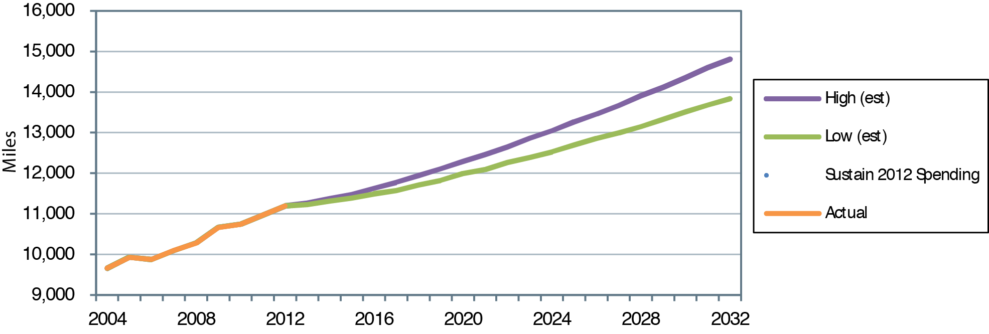
The projected guideway route miles for the Sustain 2012 Spending scenario are less than for the projected High-Growth scenario, as shown in Exhibit 9-21. (Note that TERM's projections of guideway route miles for the Sustain 2012 Spending and Low-Growth scenarios are nearly identical.) Commuter rail has substantially more guideway route miles than heavy and light rail, making accurate projections of total guideway route miles for all rail modes difficult; therefore, the historical trend line is not provided.
TERM's expansion projections of stations by scenario needed to preserve existing transit assets at a condition rating of 2.5 or higher and to expand transit service capacity to support differing levels of ridership growth (while passing TERM's benefit-cost test) are presented Exhibit 9-22. TERM's Low-Growth estimates generally are in line with the historical trend, indicating that expansion projections of stations under the Low-Growth scenario could maintain current transit conditions.
Exhibit 9-21 Projection of Guideway Route Miles by Scenario1
1Data through 2012 are actual; data after 2012 are estimated based on trends.
Source: Transit Economic Requirements Model.
Exhibit 9-22 Projection of Stations by Scenario1
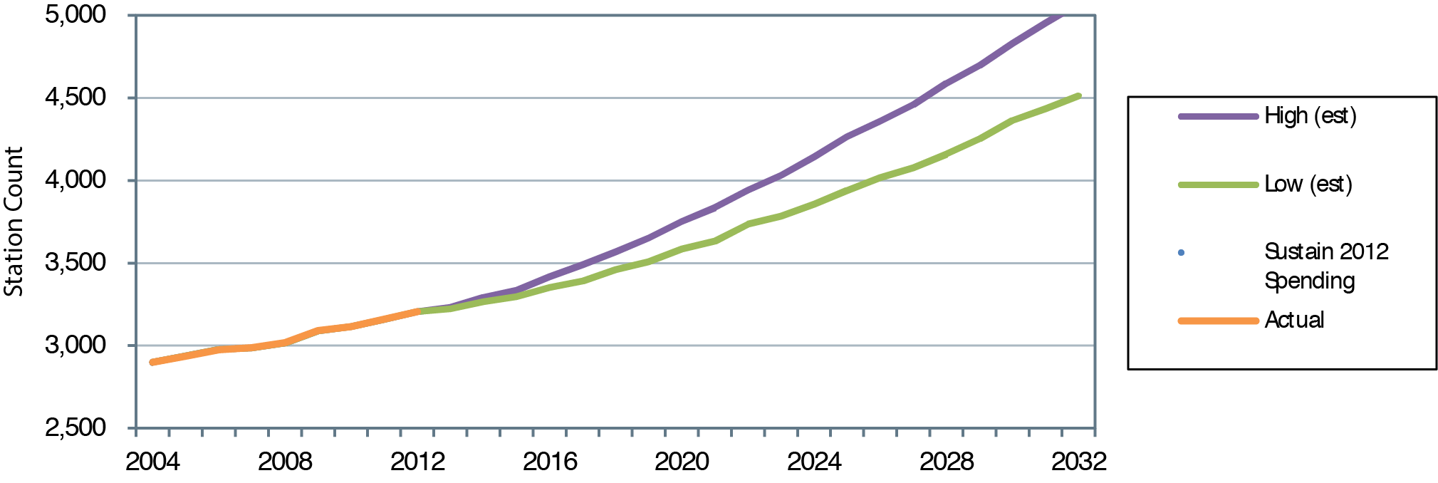
1Data through 2012 are actual; data after 2012 are estimated based on trends.
Source: Transit Economic Requirements Model.
For each scenario, TERM estimates future investment in fleet size, guideway route miles, and stations for each of the next 20 years. Exhibit 9-23 presents TERM's projection for total fixed guideway route miles under a Low-Growth scenario by rail mode. TERM projects different investment needs for each year that are added to the 2012 actual total stock. Heavy rail's share of the projected annual fixed guideway route miles remains relatively constant over the 20-year period, while the amount of fixed guideway route miles increases slightly for light and commuter rail.
Exhibit 9-23 Stock of Fixed Guideway Miles by Year Under Low-Growth Scenario, 2012—2032
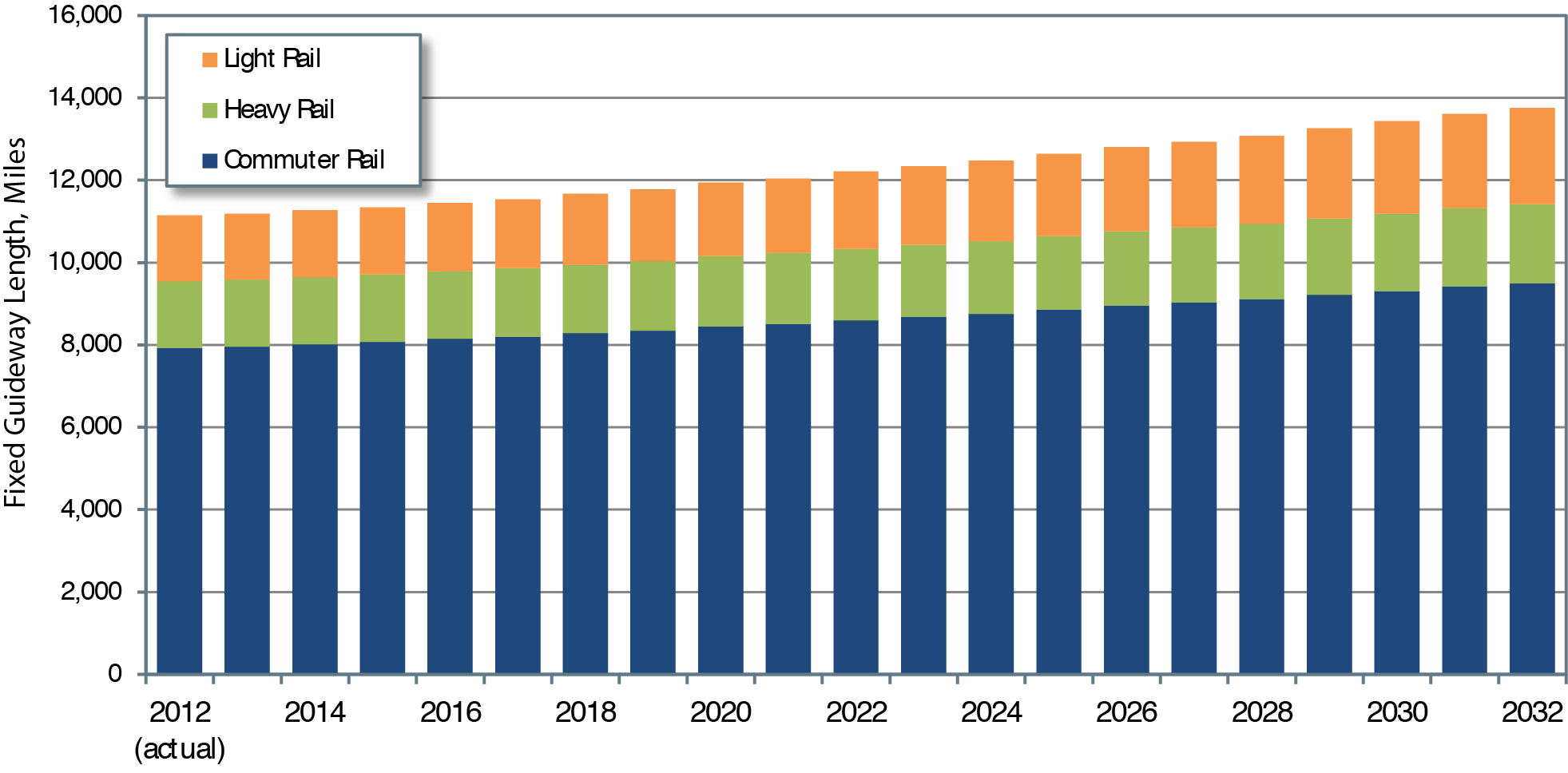
Source: Transit Economic Requirements Model.
i Subject to some limitations (e.g., agencies must surpass a minimum vehicle occupancy standard before being eligible for expansion investments). ↑