< Previous | Table of Contents | Next >

4.0 VALIDATION OF MATHEMATICAL MODELS

Validation of the mode choice models presented in the previous section is provided here through the discussion of the validation methodology (Section 4.1) and the results (Section 4.2). The reduced models will be used in a more practical sense to predict future mode choice within a transportation modeling framework as it contains only readily available input variables identified as having an influence on mode choice. Thus, all validation procedures were conducted on the reduced set of models to assess their predictive ability.

4.1 Methodology

Validation of the long-distance passenger travel modal choice models was conducted by testing the models on long-distance travel survey data. The same 2001 NHTS dataset used for model calibration was also used for model validation. One common method for validating transportation models is holdout validation where the dataset of long-distance trips is divided into two non-overlapping parts; one solely used to develop and calibrate the models and another for validating the models. This approach is used to determine if over-fitting of the model is present and provides accurate estimates for the predictive performance of the models. The downside to this approach is that it does not use all the available data. Given the limited number of long-distance trips in the 2001 NHTS and the fact that the trips were segregated by trip purpose (i.e., business, personal business, and pleasure) in order to account for the differences in mode choice by trip purpose, the holdout method was not preferable. In addition, results from holdout validation are highly dependent on the choice for the calibration/validation split. This has the potential to lead to skewed results in terms of poor prediction performance if data in the validation set that may be valuable for calibration is held out in the validation set (Refaeilzadeh, 2009). To deal with these challenges and to utilize all the NHTS data, the mode choice models were validated with a technique called k-fold cross-validation.

Cross-validation is a statistical technique for assessing how the results of the statistical model will generalize to an independent dataset. Holdout validation, described above, is the most basic form of cross-validation. In k-fold cross validation, the data is first partitioned into k equally (or nearly equally) sized segments, or folds. Then, k iterations of calibration and validation are performed such that a different fold of the data is held out for validation while the remaining k-1 folds are used to calibrate the model within each iteration. The value of k is usually dependent on the size of the dataset. Small values of k (e.g., 2 or 3) lead to calibration datasets that are not as close to the full dataset size which is not desirable while extremely large values of k increase the overlap between calibration datasets across iterations and lead to small validation datasets which could result in less-precise predictions. General consensus in the data mining and model fitting community is that k = 10 is a common choice that balances these factors (Refaeilzadeh, 2009).

For this research, 10-fold cross-validation was conducted separately to validate each of the three multinomial mode choice models (one for each trip purpose). For example, the number of business trips (10,008) was randomly divided into ten segments of approximately 1,001 long-distance trips. In the first iteration, one segment was withheld as the validation dataset while a multinomial logit model was fit to the other nine segments. Then, the fitted model was applied to the validation dataset (i.e., predicted probabilities for each mode of transportation were calculated for each trip in the validation dataset). Using the coefficients of the predictor variables, the model predicts the probability that the given traveler for each trip would choose each of the four mode choices. For example, on a given trip where private vehicle was the actual mode of choice, the probability of taking a private vehicle, air, bus, and train from the model might be 70 percent, 20 percent, 3 percent, and 2 percent, respectively. Aggregate mode shares were calculated by summing the calculated probabilities for each trip record in the validation dataset. These were compared against the observed aggregate mode shares of the validation dataset in order to observe how well the model could replicate the observed mode shares. This process was repeated nine times, each time choosing a different segment of the data to be held out as the validation dataset. Once all iterations were complete, the comparison of predicted versus observed aggregate mode shares were combined across the ten iterations and statistics summarizing the predictive ability of the model were calculated.

4.2 Results

For each of the ten iterations in the 10-fold cross validation, the aggregate mode shares across all trips in the validation dataset were calculated for each mode by summing the calculated probabilities for each trip record. These were compared against the aggregate mode shares of the dataset in order to observe how well the model could replicate the observed mode shares. The results of this comparison across the ten iterations are shown in Table 4-1 for each trip purpose.

Table 4-1. Comparison of Actual and Model-Predicted Aggregate Mode Shares by Trip Purpose.
Trip Purpose	Actual Mode	Unweighted Number of Trips	Model Predicted Mode: Personal Vehicle	Model Predicted Mode: Air	Model Predicted Mode: Bus	Model Predicted Mode: Train
Business	Personal Vehicle	8,445	93	5	1	2
Business	Air	1,244	31	66	1	2
Business	Bus	105	70	15	14	1
Business	Train	214	90	6	1	2
Pleasure	Personal Vehicle	13,438	95	4	1	0
Pleasure	Air	1,202	39	59	1	1
Pleasure	Bus	203	68	2	29	1
Pleasure	Train	62	79	14	6	1
Personal Business	Personal Vehicle	3,245	96	3	1	0
Personal Business	Air	186	48	49	3	1
Personal Business	Bus	116	36	2	62	0
Personal Business	Train	14	80	16	3	1

Notes: Shaded Cells represent percentage of trips where actual and model-predicted modes agree. Due to rounding, some row percentages do not add exactly to 100%.

For business travel, both the personal vehicle and air modes show predicted probabilities that indicate the models are highly predictive (93 percent agreement for personal vehicles and 66 percent agreement for air), as evidenced by the relatively low of number of “wrong” predictions. This reinforces the effects observed in the marginal and raw coefficient estimates for the business travel model presented and discussed in Section 3.6, where personal vehicle and air travel display several clear trends that are highly statistically significant. However, bus and train travel do not show the same high level of predictive ability (14 percent for bus and 2 percent for train).

The results for pleasure and personal business are similar to that of business trips. Note that these two models predict the likelihood of actually using a personal vehicle very well (95 percent for pleasure trips and 96 percent for personal business trips). Air travel is correctly predicted 59 percent of the time for pleasure trips and 49 percent for personal business trips. A larger percentage of bus trips are predicted correctly (29 percent for pleasure trips and 62 percent for personal business trips). However, train travel is predicted poorly for all three trip types.

Figure 4-1 shows the distribution of the predicted aggregated mode shares relative to the observed aggregated mode shares by iteration for each mode of transportation for business trips. Figure 4-2 and Figure 4-3 show the same information for pleasure and personal business trips, respectively. These graphs are useful for assessing the variability in results across the iterations of the cross-validation. From the figures, the following observations can be made concerning the proportion of predicted mode shares relative to the observed mode shares across iterations:

A bar chart plots values in percent over iteration count for each of four travel modes. For personal vehicle mode, the plot shows a value of 93 percent for iteration 1, drops to 92 percent for iterations 2 and 3, increases to 93 percent for iteration 4, and oscillates between these two values to end at a value of 93 percent for iteration 10. For air mode, the plot shows a value of 62 percent for iteration 1, and trends upward to a value of 70 percent for iteration 4, then oscillates below this value to end at a value of 60 percent for iteration 10. For bus mode, the plot shows a value of 18 percent for iteration 1 and swings downward to a value of 1 percent for iteration 3, swings upward to a value of 16 percent for iteration 5, oscillates below this value through iteration 9 and swings upward to end at a value of 35 percent for iteration 10. For train mode, the plots shows value of 2 percent for iteration 1, increases to a value of 3 percent for iteration 2 and then drops to a value of 2 percent through iteration 9, ending at a value of 3 percent for iteration 10.

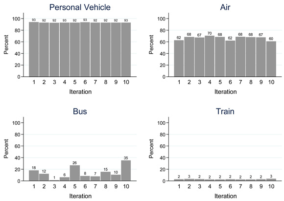
Figure 4-1. Distribution of Predicted Aggregated Mode Shares Relative to Observed Aggregated Mode Shares Across Iterations by Mode Choice (Business Trips).

A bar chart plots values in percent over iteration count for each of four travel modes. For personal vehicle mode, the plot shows a value of 96 percent for iteration 1, swings downward to a value of 94 percent for iteration 4, and increases to 95 percent through iteration 10. For air mode, the plot shows a value for iteration 1 at 62 percent, drops to 56 percent for iteration 2, increases to 60 percent for iteration 3 and drops to 54 percent for iteration 4. The oscillation between these values continues through the iterations, ending at a value of 57 percent for iteration 10. For bus mode, the plot shows a value of 47 percent for iteration 1, swings downward to a value of 19 for iteration 3, swings upward to a value of 28 percent for iterations 5 and 7 before dropping to a value of 12 percent for iteration 8 and swinging upward to end at a value of 40 percent for iteration 10. For train mode, the plot shows a value of zero for iteration 1, climbs to a value of 2 percent for iteration 3 and oscillates in this range to a value of 4 percent for iteration 7, and trails of to zero for iteration 10.

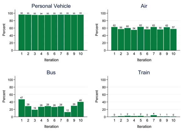
Figure 4-2. Distribution of Predicted Aggregated Mode Shares Relative to Observed Aggregated Mode Shares Across Iterations by Mode Choice (Pleasure Trips).

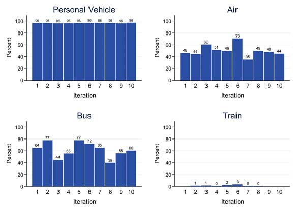
Figure 4-3. Distribution of Predicted Aggregated Mode Shares Relative to Observed Aggregated Mode Shares Across Iterations by Mode Choice (Personal Business Trips).

Results are consistently high for personal vehicle travel across all three trip purposes;
Results for air travel are consistent for business and pleasure travel but are more variable for personal business travel due in most part to the smaller number of personal business trips;
The predictive ability for bus travel varies depending on the iteration for all three trip purposes due mainly to the small number of bus trips in the NHTS; and
Train travel is consistently poorly predicted across iterations for all trip purposes.

The results of the cross-validation show that the models predict personal vehicle and air travel well. The high predictive power coupled with the consistency of results across iterations implies that the logistic regression models are not over-fit. However, the models don’t fare as well for bus and train passenger travel. When bus and train were actually used, the model most frequently predicted personal vehicle. This is most likely the product of low respondent observation counts; the models do not have the same data granularity to generate predictions as with personal vehicle and air travel. Even after accounting for survey weights, bus and train travel comprise such a small proportion of overall observations that any survey and sample bias are significant risks. The low number of observations makes it very difficult to determine those factors that influence a long-distance traveler’s decision of taking personal vehicle versus taking the bus or train. For business travel in particular, the types of persons that choose to take bus or train modes are likely to be highly variable which compounds this issue.

In order to determine which factors influence long-distance passenger travels to choose bus or train travel, more data will be needed. This will be challenge given that the long-distance trip frequency in general is low for the majority of U.S. households. The 2001 NHTS long-distance sample shows that about one-half of all surveyed households did not take long-distance trips (defined by distances of 50 miles or more) during their assigned four-week travel period. The difficulty in capturing these long-distance trips is only going to become greater as the U.S. and the rest of the world are experiencing shifts in travel behavior due to the rise of the internet, economic crisis, terrorism, and other factors. The bottom line is that although it is difficult to get survey data using traditional sampling designs such as those used for the ATS and NHTS, it is even more difficult to get data on bus and train travel. In the 2001 NHTS, only three percent of all long-distance trips were taken by bus and train. The same holds true for the 1995 ATS where about two percent of all long-distance trips were taken by bus and less than one percent by train.

In order to gather more data on bus and train long-distance travel, the research team believes that the sample design and data collection techniques for future national household long-distance transportation surveys needs to be modified to address these concerns. The following are some possible improvements to the design that would result in more long-distance passenger travel data. These are presented as ideas that would warrant more research to determine their feasibility and value to long-distance travel surveys. Each of them has inherent advantages and disadvantages that would need to be explored. These potential improvements are a few of the long-distance travel survey items that are currently being investigated by the research team as part of a separate project with FHWA focusing on designing a completely new approach for a long-distance travel survey instrument.

Abandon household sample frames: Instead of relying solely on household sample frames to form the sample, one idea would be to sample trips in process. Travelers could be intercepted at train or bus stations as well as airports. In addition, a sample could be made of all ticket purchases. This would be a form of area-based sampling with facilities or locations serving as the area of interest rather than households.
Use of Multi-frame Sampling Designs: Dual-frame or multi-frame sampling designs for surveys primarily seek to prevent noncoverage bias. As the U.S. population becomes increasingly mobile and the emergence of positioning- and event-related technology advances, new technology-based frames are becoming more available such as those based upon Facebook, Twitter, Four Square, etc. These technologies tend to focus more on individuals rather than households. In these situations, the use of a multi-frame design may become more appealing and would be worth additional investigation.
Collect data more frequently: Event driven data collection such as pulse surveys could be used to capture more long-distance trips as they are occurring. Future surveys, especially those attempting to characterize rare events, have the novel capability of being designed around “event-driven” data collection. This concept involves detecting and collecting information on household travel events in a passive manner, by accessing data sources that are made available to the survey upon receiving explicit informed consent of the survey participants to do so. Example data sources include cell phone tracking information and social media postings (Facebook, Twitter, etc.). For example, if a survey participant’s cell phone (or the cell phone of an individual within a selected household) is noted to have moved a distance that exceeds a given threshold, this finding would indicate that a long-distance travel event occurred. This concept is known as “geo-fencing.” This concept could leverage technology to trigger a survey once a participant travels a certain number of miles. In addition to capturing data on long-distance trips, this method would effectively shorten the recall period for the survey participant which could help to reduce recall bias.
Use of social media to connect to participants: Social media data could be mined to identify past, current, and future long-distance trips. It could also be used for self-reporting of trip events and/or as a data collection mechanism.