

3.0 MATHEMATICAL MODELS FOR PREDICTING MODE CHOICE
This section discusses the development of the mathematical models to predict mode choice starting from the input data sources and going through the model results. Section 3.1 discusses the main data source, the 2001 NHTS. Section 3.2 presents additional sources used to supplement the NHTS. A summary of predictive factors used in the mode choice modeling is given in Section 3.3 followed by a descriptive analysis of these factors in Section 3.4. The statistical background and methodology for the models is presented in Section 3.5 followed by the results in Section 3.6. Finally, a discussion of the results is presented in Section 3.7.
3.1 2001 National Household Travel Survey
The 2001 NHTS is a national survey of daily and long-distance travel. The survey includes demographic characteristics of households, people, vehicles, and detailed information on long-distance travel for all purposes by all modes. NHTS survey data are collected from a sample of U.S. households and expanded to provide national estimates of trips and miles by travel mode, trip purpose, and a host of household attributes. According to BTS, the NHTS provides the only authoritative source of information at the national level on the relationships between the characteristics of personal travel and the demographics of the traveler. In addition to providing the first comprehensive look at travel by Americans, the 2001 NHTS also incorporated additional enhancements to previous sample designs (e.g. 1995 ATS and prior Nationwide Personal Transportation Surveys (NPTS)). For example, long distance travel was expanded to include trips as short as 50 miles and, for the first time, included trips made for the purpose of commuting to work – often overlooked segments of personal long-distance travel (BTS, 2003).
The NHTS collected travel data from a national sample of the civilian, non-institutionalized population of the United States. Sampling was done by creating a random-digit dialing list of telephone numbers. An eligible household excludes telephones in motels, hotels, group quarters, such as nursing homes, prisons, barracks, convents, or monasteries, and any living quarters with ten or more unrelated roommates (FHWA, 2004).
There were approximately 66,000 households in the final 2001 NHTS dataset. About 26,000 households were from the national sample, while the remaining 40,000 households were from nine add-on areas. The nine add-on areas were: Baltimore, Des Moines, Hawaii, Kentucky, Lancaster PA, New York State, Oahu, Texas, and Wisconsin. The final datasets contained about a quarter-million daily trips and 45,165 long distance trips.
NHTS data was obtained by using Computer-Assisted Telephone Interviewing (CATI) technology. Each household was assigned a specific twenty-four hour “Travel Day” to record daily travel by all household members. In addition, a twenty-eight day “Travel Period” was assigned to each household to collect longer-distance travel. Long-distance trips in the 2001 NHTS are defined as trips of 50 miles or more from home to the farthest destination traveled that started and ended within the four-week travel period. Data collected on long-distance trips includes:
- Purpose of the trip (pleasure, business, personal business);
- Means of transportation used (car, bus, train, air, etc.);
- Day of week when the trip took place;
- If a personal vehicle trip:
- Number of people in the vehicle;
- Driver characteristics (age, sex, worker status, education level, etc.);
- Vehicle attributes (make, model, model year, amount of miles driven in a year); and
- Location of overnight stops and access/egress to an airport, train station, bus station, or boat pier.
Furthermore, the 2001 NHTS data contains data on the following:
- Household data on the relationship of household members, education level, income, housing characteristics, and other demographic information;
- Information to describe characteristics of the geographic area in which the sample household and workplace of sample persons are located;
- Public perceptions of the transportation system;
- Internet usage; and
- Information on each household vehicle, including year, make, model, and estimates of annual miles traveled.
For all of its strengths, there are some drawbacks to the 2001 NHTS. Each traveler provided data about household and trip characteristics; however, many data that may be important for long-distance travel mode choice decisions were not in the scope of the 2001 NHTS data collection. Examples of data not included in the NHTS data are travel costs and travel time as well as information that would identify the traveler’s household or workplace information. Specifically, geographical information at the origin and destination of trips is aggregated to protect the confidentiality of respondents. Trips in the survey are only identified on both the origin and destination side by state and Metropolitan Statistical Area (MSA). Furthermore, about half the long-distance trips do not have origin or destination information below the state level. This is because either trips do not originate or destinate in an MSA or the MSA is too small in terms of population density to publish it in the dataset for confidentiality reasons. Fortunately, the research team obtained a separate file from FHWA that contained the 5-digit ZIP Code of each household in the survey. This research assumes that each trip originated at the household. Having this information was critical in assessing the availability of transportation infrastructure relative to the origin of the trip. To compensate for other variables that may be important for long-distance mode choice but not present in the NHTS, outside data sources were identified that would provide such variables (or suitable proxies for the variables) that could supplement data from the NHTS.
Another limitation of the 2001 NHTS dataset is that although each traveler provided information about the mode that they used, they did not provide information about other alternative modes or the traveler’s reason for selecting a specific mode of travel over another mode. As will be discussed more in Section 3.5, this fact played a significant role in determining the type of multinomial logistic regression model to use to predict mode choice.
Another rich source of long-distance travel data is the 1995 ATS. This was a panel survey conducted by BTS in 1995 which collected information from approximately 80,000 households about their long-distance travel through 1995. Although the ATS has a larger number of long-distance trips compared to the 2001 NHTS, the 2001 NHTS was preferred over the 1995 ATS mainly because the NHTS contains more recent information. This was important as the data from the 2001 NHTS is already ten years old. In addition, the ATS also suffers from the same lack of reported geographic detail at the origin and destination side of trips to protect confidentiality that the NHTS does. While the research team was able to acquire five-digit ZIP Code information on the surveyed households for the NHTS to help with land-use and other variables, this information was not available from the ATS. For these reasons, the ATS was not considered in the model development.
The 9/11 terrorist attacks occurred in the midst of NHTS data collection efforts, and the potential impact of this event on data collection and travel behavior was investigated as a part of the review of this data source. Many studies note that air travel experienced a large initial usage “shock” in the immediate aftermath of the attacks followed by an almost complete recovery in consumer demand by the end of the NHTS study period. There is little evidence that NHTS data suffers from a severe deficiency of air travel observations due to any effect of 9/11, since airline travel statistics published by Research and Innovative Technology Administration (RITA) show that the total annual number of passengers enplaned by domestic carriers was only slightly lower in 2002 than in 2001. However, in order to capture any potential effect on travel behavior caused by the 9/11 attacks, a dichotomous variable was added to track any effect caused solely by travel dates that occurred after the event.
3.1.1 Trip Purpose and Mode Choice
A separate model was developed for each trip purpose: business, pleasure, and personal business. Business trips are ones where a business function is the primary purpose (i.e., to attend a conference, business meeting, or other business function other than commuting to and from work). Other non-business activities can occur as long as the trip is primarily for business. Pleasure trips include trips for vacations, visiting friends and relatives, sightseeing, and outdoor recreation. Personal business trips include trips for medical visits, trips to attend funerals, weddings, and other events. The “other” trip purpose was excluded from the analysis, leaving business, pleasure, and personal business as the three trip purposes used in the modeling.
The modes personal vehicle, air, bus, and train were used in the modeling. The modes “ship” and “other” were not included in the analysis because the number of data points was minimal. A personal vehicle can be a passenger car, sport-utility vehicle, van, or other vehicle owned by the household. Personal vehicles are attractive choices to long-distance travelers in that one can travel from origin to destination and still have a vehicle to use at the destination, travelers have more privacy, and they can have a more flexible schedule. However, personal vehicles can be a slower mode of travel. Vehicles such as taxis, limousines, and other car services were not included as they fell into the “other” mode category and represented a very small portion of the sample. The air mode is a faster transportation alternative but the cost for this alternative is relatively high. Bus and train modes are both ground modes that are usually slower modes which may need to stop at many stations before arriving at a destination. However, they are attractive options for those who do not own a personal vehicle or for those traveling in large groups. For each long-distance trip, the dataset contains information on all travel modes taken on the outbound side of the trip (origin to farthest destination) as well as the return trip. Multiple modes may be taken to get from the origin to destination and these are recorded in the NHTS. For example, a traveler could take a taxi to the airport, a plane to the destination city, and then a rental car to the final destination. For each trip, the NHTS identifies one mode (MAINMOD2) as the main mode that the traveler used most to get to the destination. In the previous example, the main mode would be “air”. In this research, this variable identifies the mode of travel for the trip and is the only one considered in the modeling. Although it is possible for the main mode of transportation on the return trip to be different than that on the outbound side of the trip, this research focuses only on the one-way portion of the trip from origin to farthest destination.
3.1.2 Prediction Factors from 2001 NHTS
Variables used in this research came from trips in the national NHTS sample as well as those in the add-on samples. There were many variables present in the NHTS dataset but only a subset was used for model development. Those used for the modeling include ones that were identified from the literature and practice review as well as those that showed a significant correlation with mode choice in exploratory analysis. Some of the variables used were taken directly from the NHTS data files while others, as noted below in the variable descriptions were modified or redefined slightly to reduce the dimensionality of the variable. Variables used in the modeling from the NHTS include:
- Total income of all household members: Income is a very important factor for people who travel long distances. In regards to income, Mallett (1999a) found that about two-thirds of people in low-income households did not make a single long-distance trip in 1995 with the most important limiting factors being the availability of a vehicle. Moreover, lower income groups were found to be much more likely to travel by automobile or bus when compared to other income groups (Georggi and Pendyala, 1999). Air travel was a more popular choice for long-distance travel as income levels increased. Household income was separated into four levels: households making less than or equal to $30,000 annually, households making over $30,000 and up to $60,000 annually, households making over $60,000 and up to $100,000 annually, and households with an income greater than $100,000 annually. An indicator variable was created for each of the four household income levels.
- Age of traveler: Age is a factor that may impact mode choice. Georggi and Pendyala (1999) found that the elderly are significantly more dependent on the bus mode than the rest of the population. Also, the automobile mode share diminishes significantly for people over 75 years of age as the airplane and bus are used instead of the automobile more frequently (Georggi and Pendyala, 1999).
- Employment status of respondent: An indicator of whether the traveler is employed. This variable is included on the hypothesis that employed travelers are likely to take more expensive modes of transportation than those who are unemployed.
- Population per square mile – block group for household: This is a measure of land-use on the origin side of the trip. Travelers who live in heavily populated areas would be more likely to have access to different transportation infrastructures and also to route alternatives that could impact travel mode choice.
- Number of vehicles in household: This variable shows the potential of a household to have a variety of personal vehicles. Households with large number of vehicles may have vehicles of different types which would allow selection based on trip purpose. For example, large families with a minivan or SUV traveling a long distance might be more inclined to take a personal vehicle than other modes.
- Public transit use: This provides a description of the traveler’s public transit use in the last two months. This will serve as an indicator of a traveler’s familiarity and comfort level with public/commercial transportation which may have behavioral implications for travel mode choice. From the NHTS variable PTUSED, a binary indicator variable (high_PTuse) was created to identify travelers who use public/commercial transportation at a rate of more than once or twice per month versus those who use it less than once or twice per month.
- Internet use: Provides an indication of a traveler’s internet use over the last six months. Travelers who use the internet more frequently would most likely have access to detailed travel information on alternative travel modes (e.g., airline costs and schedules) which could be a potentially important determinant of using travel modes such as airlines. From the NHTS variable WEBUSE, a binary indicator variable (high_webuse) was created to identify travelers who use the internet weekly versus those who use it less frequently.
- Nights away on trip: The number of nights away on a long-distance trip impacts which mode to select. A family or group of travelers might want to spend more nights at a destination rather than many nights en route to the destination. Thus, shorter trips might be conducive to faster travel modes.
- Trip before or on/after 9/11: The terrorist attacks on September 11, 2001 occurred during the data collection for the NHTS survey (March 2001 through May 2002). The terrorist attacks played a significant role on the behavior of intercity travelers in that after 9/11, people avoided traveling by air either out of fear or because of the increasing security and the uncertainty of passenger processing times at airports. The variable is an indication as to whether the trip occurred after 9/11 or before 9/11.
- Race of traveler: Differences in race may affect mode choice for long-distance travel. Indicator variables were created for each of the following races: white, African-American, Asian, Hispanic, and other.
- Origin to destination route distance: Route distance is a critical factor when choosing mode choice. Longer-distance travel will most likely encourage a traveler to select a faster mode. As trips become longer, the probability of taking personal vehicle or other ground forms of transportation should be reduced.
- Number of people on trip: The greater the number of people on a trip, the greater the travel expense. Thus, families and groups of travelers in large numbers may be more likely to choose personal vehicle or perhaps bus as compared to more expensive options such as air.
- Location of household: This is another measure of land-use on the origin side of the trip. Travelers who live in an urban area would be more likely to have access to different transportation infrastructures and also to route alternatives that could impact travel mode choice more so than in rural areas.
- Trip includes weekend: Travelers who travel during the week or on short weekend trips may prefer a faster transportation mode such as air because they need to return for work. For longer weekend trips, a slower transportation method may be preferred as travelers may have more time to spend and can do so at a lower cost.
Shortly after model development and the initial draft of the technical report, FHWA and the research team discussed the list of variables used from the NHTS to predict mode choice. FHWA expressed concern that although certain variables may play a role in determining a traveler’s mode choice, it might prove difficult to obtain valid estimates for these variables when using the model to forecast mode choice within the national transportation modeling process. These variables are: 1) a measure of a traveler’s public transit use; 2) a measure of a traveler’s internet use; 3) the number of nights away on a trip; and 4) an indicator of whether the trip involved a weekend. The research team believes these variables are very informative and have an effect on the choice of transportation mode. However, the team also understands that the variables are useless in the model if no practical inputs can be easily obtained (i.e. from census data) without conducting another large scale travel survey. As a result, the research team presents in Section 3.6 both a full mode-choice prediction model with all the inputs identified in this section as well as a reduced prediction model that removes these variables.
In addition, FHWA expressed policy concerns with including the race variables in the model. Although the inclusion of race as a demographic variable in economic studies is quite common and has even been used in past long-distance travel mode choice studies (Georggi and Pendyala, 1999, Rasmidatta, 2006), the research team acknowledges and understands the policy concerns and implications and thus has not included the race variables in the reduced prediction model. Their effect is still explored in the full model.
Version 4.0 (July 2005) of the 2001 NHTS data was used in the analysis and model formulation. Both the 2001 NHTS long-distance trip dataset and the dataset of replicate weights were obtained from the NHTS Data Center located on the NHTS website http://nhts.ornl.gov/download.shtml. In addition, the United States Department of Transportation (USDOT) version of the 2001 NHTS household data (containing more detailed geographic information on survey households) was provided by Oak Ridge National Laboratory through FHWA.
3.2 Data Sources to Supplement the 2001 NHTS
Although the NHTS gives detailed information on individual and trip level demographic information, several variables from external data sources were included in the model. These variables, accounting for economic and environmental factors, are not present in the NHTS data but were identified in the literature review as determinants of individual travel choice mode. Two main factors governing individual choice of travel mode that these variables particularly seek to include are the economic burden of particular modes of travel as well as the availability and access to transportation infrastructure. Along with demographic information, this additional information can serve as a means to increase the resolution of predictions about travel mode choice based on observed data.
3.2.1 Economic Factors
The research team acknowledges the importance that travel cost plays on a traveler’s choice of transportation mode. Unfortunately, the NHTS did not collect data that characterize the different travel costs associated with the available mode choices. To overcome this problem, previous research (Ashiabor et al, 2007 for example) has developed synthetic travel cost estimates for each mode of transportation between major origin/destination pairs using such resources as published airline fares, rail and bus fare schedules, and mileage between various geographic destinations. In addition, assumptions were made as to the extra costs incurred on the trip (access/egress transportation, overnight lodging, etc.). This provided a generalized cost estimate for each trip. The resources available to the current research project described in this report did not allow for this type of data collection and use. Furthermore, this method involves making a lot of assumptions about the costs of travel that the research team did not feel warranted making. So, as an alternative, this research focused on creating a generalized cost component for the model based on major economic indicators related to travel at the time of the long-distance trip. This section describes that process.
The first group of non-NHTS variables included in the model seeks to capture any existing economic effects that drive the actions of consumers of different modes of travel. Each potential mode of travel for a long distance trip has its own economic burden; for example, driving a personal vehicle incurs the cost of paying for gas and any risk of repairs while flying on a domestic airline incurs the cost of a ticket. These factors, in conjunction with demographic data such as income levels, serve as deterrents or incentives for individuals to choose one mode of travel over another. The economic effect of cost is not entirely captured through income level – if the price of an airline ticket becomes sufficiently low, an increasing portion of consumers will choose to substitute airline travel for personal vehicle travel even when holding income level constant. Listed below are the variables included that address these price changes and the resulting effect they have on the desirability of certain travel modes.
- Air Travel Price Index: The Air Travel Price Index (ATPI) is a statistical index that denotes the relative price levels of airfares faced by consumers over time. The Research and Innovative Technology Administration (RITA) of USDOT compiles this index, beginning in the first business quarter of 1995, by matching identical routings and airfare classes and the changes in their costs over time at quarterly intervals. Three different types of ATPI measurements are provided by RITA depending on the origin of the flight; this analysis uses only the U.S.-origin ATPI in an attempt to limit any foreign airfare price effects. RITA also provides the average airfare price over this time interval, but the price index is advantageous to a national average due to direct routing-price pair wise comparisons used in its calculation which may differ over domestic locations (an average masks potential local differences). The index takes value 100 in the first quarter of the first year (1995), and then changes based on the relative magnitude of increase or decrease in overall airfare prices in subsequent quarters. The change in the value of the ATPI over time is shown below in Figure 3-1:
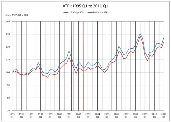
Figure 3-1. Plot of Air Travel Price Index from 1995 to 2011.
The red vertical bars denote the range of travel dates observed in the NHTS sample based on the travel periods for each respondent; the relevant airfare price levels faced by consumers over this time period vary considerably, chiefly due to the effect of the 9/11 attacks on the air travel industry and demand for air travel. This variable is intended to provide a measure of consumers’ price thresholds for air travel modes, with the expected model effect being an increase in the relative price of airline travel corresponds with a decrease in the likelihood of choosing air travel as the desired mode. Also, changes in the price of airfare may be correlated with increased chances of choosing other modes as consumers substitute towards less expensive alternatives. The price of the index was recorded at the time of the travel period for each respondent. Although the purchase time of the air transportation would be preferable, it was not available in the NHTS data.
- Consumer Price Index Private Transportation Component: Similar to the price of airfares, economic incentives in mode choice will exist for the use of private transportation. Using the Consumer Price Index (CPI) commodity category for private transportation published the U.S. Bureau of Labor Statistics (BLS), the model can account for changes in the price of owning and operating a personal vehicle and assess any effect this has on the likelihood of choosing a transportation mode for long distance travel. The CPI for private transportation is calculated using the relative price changes in a variety of personal vehicle ownership cost categories and relative importance weights associated with each cost, with the index taking the baseline value of 100 for the years 1982-1984. The costs included in the aggregate private transportation index include:
- the purchase and lease price of new and used motor vehicles;
- the price of fuel;
- the price of motor vehicle parts and equipment;
- the price of vehicle maintenance and repair; and
- the price of motor vehicle insurance and other fees.
- Consumer Price Index Public Transportation Component: The BLS also publishes a monthly CPI that captures the general price levels of available public/commercial transportation options. Consumers of public/commercial transportation may be especially susceptible to changes in price in determining their mode choice for longer distance trips, as there are several disincentives to using public/commercial transportation over personal or air travel (time and privacy costs). The CPI for public transportation is calculated similarly to the methods described above for private transportation. The public/commercial transportation index also takes the baseline value of 100 for the years 1982-1984 and includes price change information on the following types of transportation:
- Intercity bus fare;
- Intercity train fare;
- Ship/ferry fare; and
- Intra-city mass transit.
Other measures of the potential economic burden of specific travel modes were considered and excluded from the model’s analysis based on analyses of their overall effect. Individual indices for both Amtrak train fares as well as cross-country bus fares were initially included in the model, but were found to be insignificant predictors. The CPI for public/commercial transportation yields virtually the same model effects, so these indices were excluded in order to avoid over-specifying the model and to avoid multicollinearity issues in the model fit. The index for airline prices was not highly correlated with either CPI measure; additionally, consumer demand for airline tickets is much more sensitive to price changes than public/commercial transportation. Also, measures of general economic conditions were initially included as potential indicators of the willingness of travelers to choose “high end” travel options during periods of prosperity; among these was the University of Michigan’s Consumer Sentiment Index which tracks the general level of consumer confidence in the economy at a given point in time. These were also found to be unnecessary, as all of the price effects’ impact on transportation mode choice was captured in the included indices and the effect of other economic predictors on the model’s overall fit was minimal.
3.2.2 Availability of Transportation Infrastructure
A second group of variables was also included in the model analysis in order to account for factors outside those captured in the NHTS. A traveler’s mode choice is likely to be affected not only by the price of a given service, but also its availability. A key component in this availability is proximity to points of access to a transportation option for both the primary and any secondary modes of trip travel. For example, a traveler’s propensity to choose airline travel will not only be affected by the location of the airport itself, but also by secondary transportation options to and from the airport such as intercity rail. Some modes of transportation may be limited or may not be available in some areas, making personal vehicle the only feasible option for long distance travel. To account for any effect availability and access has on final travel mode choice, the model included variables that measure the level of transportation infrastructure and its proximity to the residence of travelers.
The locations of major hubs for various modes of transportation across the United States were assimilated to create a single set of transportation infrastructure sites. The database includes the locations of airports, standard rail stations, transit rail stations, and large bus depots. The airport locations were acquired from the National Transportation Atlas Database 2011 (NTAD2011) and represent all landing facilities in the U.S., as provided and maintained by the Federal Aviation Administration. The airports were filtered such that only those that would be used by a typical traveler were included. All private airports, heliports, ultralight ports, balloon ports and glider ports were excluded. In addition, those airports with no commercial activity and no central tower were assumed to be too small to be used by a casual traveler. Figure 3-2 shows the locations of the airports considered in this study.
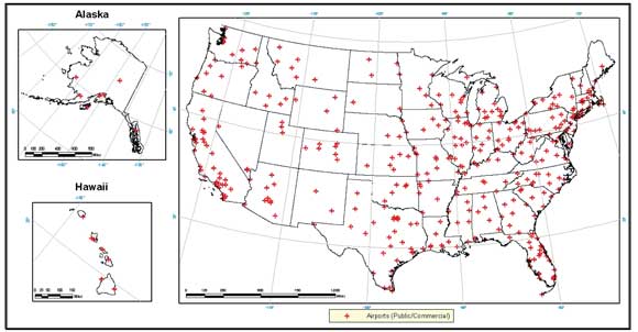
Figure 3-2. Locations of Large, Public-Use Airports from NTAD2011.
Both standard rail (i.e. Amtrak) and transit rail (e.g. light rail, subways, etc.) stations were acquired from NTAD2011 and included in the database (Figure 3-3 and 3-4). Noticeably missing from the NTAD2011 transit rail data were the New York City subway system and the Long Island Rail Road (LIRR). The locations of stations contained within these systems were acquired from the Metropolitan Transit Authority (MTA) General Transit Feed Specification (GTFS) (Figure 3-5). There are several other light rail and passenger rail systems that are not included in this dataset. Many of these were constructed or brought online after the most recent date observed in the NHTS sample data (corresponding to April, 2002) and are thus not considered to create a missing data issue given that they were not available at the time. Hence, the predictive ability of the model should not be hampered significantly when trying to predict trips during the time of the NHTS. Because of this, the count of light rail stations is included in the full prediction model in order to ascertain the general effect these stations have on mode choice. The NTAD notes that it will update its database with a significant amount of light and transit rail station data in late 2011, and there are potentially some transit rail observations missing from the infrastructure database. Given the model is going to be used to predict mode choice of future trips within the construct of a national transportation framework model and the amount of missing stations unknown at this time, this variable has been removed from the reduced prediction models which will be used in the near term for prediction.
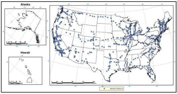
Figure 3-3. Locations of Amtrak Stations from NTAD2011.
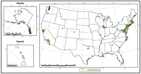
Figure 3-4. Locations of Light Rail Stations from NTAD2011.
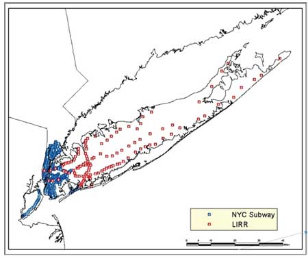
Figure 3-5. MTA NYC Subway and LIRR Stations.
While there are a vast number of single public transit bus stops throughout the country, only the major bus stations or depots were considered for this study. These stations included only major transfer or hub sites, which travelers would generally need to access for long distance travel (i.e. not intracity travel). The locations of bus stations or depots were obtained from NTAD2011 and are shown in Figure 3-6.
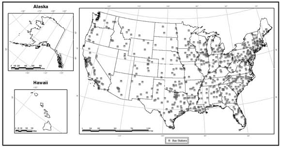
Figure 3-6. Locations of Large Bus Stations.
In order to calculate a measure of accessibility for each survey respondent, available transportation infrastructure locations were matched to each survey respondent. The highest level of geographic location information collected from the survey respondents was the 5-digit ZIP Code of residence. The 5-digit ZIP Code for each survey respondent was geocoded to the delivery-based ZIP Code centroid to represent the origin location. There were 12 ZIP Codes that could not be geocoded; two of which were not valid ZIP Codes. The remaining 10 ZIP Codes were manually assigned the data associated with the closest ZIP Code using the associated city name from the U.S. Postal Service database.
It was estimated that 25 miles was a reasonable travel distance from a respondent’s residence to a transportation hub. This distance is assumed to represent a basic awareness of local travel options by each respondent as well as the ability to reach infrastructure hubs within this distance using personal vehicles or public transit as an intermediate step in the overall trip. The counts of each type of transportation mode that fell within the buffered distance were calculated to represent the respondents’ access to alternative transportation (Figure 3-7).
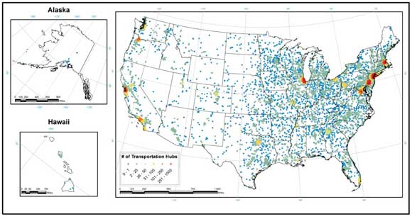
Figure 3-7. Number of Transportation Hubs Within 25 Mile Buffer for Each Survey Respondent.
Within the 25 mile buffer radius, counts of infrastructure sites were summed and included in the model as variables measuring access to different travel mode options. If travel mode choice is dependent on level of access, model results will show a significant relationship between marginal increases in the number of travel mode infrastructure sites within the buffer distance. For example, if the choice of air travel is highly dependent on access to airports, marginal increases in the number of airport sites within a traveler’s access radius (say, from 0 to 1 airport sites) should yield significantly increased probabilities of taking air travel. The final infrastructure count sums within each survey respondent’s assumed 25 mile access radius were compiled in four variables included in the model listed below:
- Count of all air travel sites;
- Count of all light and transit rail sites;
- Count of all standard rail sites; and
- Count of all bus travel sites.
The final set of variables included in the model was chosen based on the statistical considerations mentioned in the discussion above as well as a series of pair-wise and overall correlation analyses. This involved using statistical software to search out combinations of different variables for highly correlated variables, which if included in the model would essentially be duplicating the analysis of any effect on the travel mode outcome and create multicollinearity problems with the logistic regression model fits. Using traditional correlation matrices, a number of price index variables acquired from the St. Louis Federal Reserve were discarded due to their high correlations with one another. Also, a number of measurement indices of consumer confidence were found to be highly correlated with measures of price levels for public and private transport and were thus discarded from consideration. Several measures of population density, metropolitan statistical area classification, and household demographics in the original NHTS data set were also found to be correlated with one another; in all cases, only one metric was chosen to be included in the final set of analysis variables as determined by examination of the correlation matrices. If the factor chosen for the model had a significant effect on mode choice, then it was noted that the outcome may be linked to either the factor in the model or one of the excluded variables that were correlated with the factor in the model.
Additionally, some preliminary maximum likelihood models using the overall sample of data were used to assess preliminary model fit and further refine the set of variables used. Some variables that displayed mixed correlation results, such as the University of Michigan consumer demand index and the RITA price index for Amtrak fares, were found to have negligible effects on predicting probabilities in preliminary model runs and were not considered further. Statistical verification of improved model fits was observed after dropping these additional variables, and variables were further tested against preliminary model runs using sample data subset by each trip purpose.
3.3 Summary of Predictive Factors Used in Mode Choice Modeling
Table 3-1 provides a summary of the prediction factors discussed in the previous few sections that were used in the mode choice analysis. The factors are grouped by type and contain information on the coding of the categorical variables.
| Type of Factor | Factor | Description |
|---|---|---|
| Traveler Characteristics | Traveler’s Age | Integer |
| Traveler Characteristics | Household Income |
Four categorical, dichotomous variables: $0<=Income<=$30,000 (1=yes, 0=no) $30,000<Income<=$60,000 (1=yes, 0=no) $60,000<Income<=$100,000 (1=yes, 0=no) $100,000<Income (1=yes, 0=no) |
| Traveler Characteristics | Race* |
Five categorical, dichotomous variables: White (1=yes, 0=no) African-American (1=yes, 0=no) Asian (1=yes, 0=no) Hispanic (1=yes, 0=no) Other (1=yes, 0=no) |
| Traveler Characteristics | Weekly Internet Use* | Categorical (1=yes, 0=no) |
| Traveler Characteristics | Weekly Use of Public/Commercial Transportation* | Categorical (1=yes, 0=no) |
| Traveler Characteristics | Traveler is Employed | Categorical (1=yes, 0=no) |
| Traveler Characteristics | Count of Vehicles in Household | Integer (counts) |
| Land-Use Characteristics | Household in Urban Area | Categorical (1=yes, 0=no) |
| Land-Use Characteristics | Population per Square Mile of Household | Continuous |
| Trip Characteristics | Trip Occurred on Weekend* | Categorical (1=yes, 0=no) |
| Trip Characteristics | Number of People on Trip | Integer (counts) |
| Trip Characteristics | Trip Distance | Continuous |
| Trip Characteristics | Nights Away on Trip* | Integer (count) |
| Availability of Transportation Infrastructure | Count of all Airports within 25 Mile Radius of Household | Integer (count) |
| Availability of Transportation Infrastructure | Count of all Bus Depots within 25 Mile Radius of Household | Integer (count) |
| Availability of Transportation Infrastructure | Count of all Amtrak Stations within 25 Mile Radius of Household | Integer (count) |
| Availability of Transportation Infrastructure | Count of all Transit/Subway/Light Commuter Train Stations within 25 Mile Radius of Household* | Integer (count) |
| Economic | CPI for Private Transportation – Seasonally Adjusted | Continuous |
| Economic | CPI for Public Transportation – Seasonally Adjusted | Continuous |
| Economic | RITA Airline Ticket Price Index | Continuous |
| Other | Post 9/11 | Categorical (1=yes, 0=no) |
3.4 Descriptive Analysis
The final data file for the passenger choice modeling was compiled using variables from the NHTS and the supplemental data sources. Trips with missing values for any of the variables were excluded, which reduced the dataset to 28,402 long-distance trips. Table 3-2 shows the unweighted number of long-distance trips used in the modeling by trip purpose and travel mode. Note that personal business trips represent a smaller subset of the data set (11 percent of trips) relative to business and pleasure travel purposes. Also, the vast majority of survey respondents took personal vehicles on their trips (88 percent of trips), regardless of purpose. Air was chosen in about 9 percent of the trips while bus (1.5 percent) and train (1 percent) were chosen less frequently. This should yield several expected consequences in analysis, namely that the analysis model should have the most informed predictions of travel mode choice for personal vehicles given the discrepancy in the resolution of the available data. In addition, it is possible that the relative lack of responses for bus and train trips, even compared to air travel, could introduce small sample biases into predictive analyses of bus and train travel outcomes, especially for personal business trips.
| Personal Vehicle | Air | Bus | Train | Total | |
|---|---|---|---|---|---|
| Business | 8,443 | 1,244 | 105 | 195 | 9,987 |
| Pleasure | 13,416 | 1,195 | 203 | 61 | 14,875 |
| Personal Business | 3,224 | 186 | 116 | 14 | 3,540 |
| Total | 25,083 | 2,625 | 424 | 270 | 28,402 |
Table 3-3 displays the weighted descriptive statistics for each analysis variable. For each variable the mean and standard deviation (shown in parentheses) is provided for the following: (1) all trips; (2) by trip purpose across modes of transportation; and (3) by mode of transportation across the trip purposes.
| Factor | All Trips | Trip Purpose: Business | Trip Purpose: Pleasure | Trip Purpose: Personal Business | Transportation Mode: Personal Vehicle | Transportation Mode: Air | Transportation Mode: Bus | Transportation Mode: Train |
|---|---|---|---|---|---|---|---|---|
| $0<=Income<=$30,000 |
0.11 (0.00) |
0.07 (0.00) |
0.12 (0.00) |
0.18 (0.01) |
0.12 (0.00) |
0.05 (0.00) |
0.15 (0.02) |
0.09 (0.02) |
| $30,000<Income<=$60,000 |
0.32 (0.00) |
0.28 (0.00) |
0.34 (0.00) |
0.35 (0.01) |
0.33 (0.00) |
0.17 (0.01) |
0.38 (0.02) |
0.26 (0.03) |
| $60,000<Income<=$100,000 |
0.32 (0.00) |
0.36 (0.00) |
0.31 (0.00) |
0.29 (0.01) |
0.33 (0.00) |
0.31 (0.01) |
0.30 (0.02) |
0.37 (0.03) |
| $100,000<Income |
0.25 (0.00) |
0.29 (0.00) |
0.23 (0.00) |
0.18 (0.01) |
0.22 (0.00) |
0.48 (0.01) |
0.17 (0.02) |
0.29 (0.03) |
| Post 9/11 |
0.62 (0.00) |
0.64 (0.00) |
0.61 (0.00) |
0.60 (0.01) |
0.62 (0.00) |
0.60 (0.01) |
0.69 (0.02) |
0.61 (0.03) |
| African-American |
0.03 (0.00) |
0.02 (0.00) |
0.03 (0.00) |
0.05 (0.00) |
0.03 (0.00) |
0.03 (0.00) |
0.08 (0.01) |
0.03 (0.01) |
| Asian |
0.01 (0.00) |
0.01 (0.00) |
0.02 (0.00) |
0.02 (0.00) |
0.01 (0.00) |
0.02 (0.00) |
0.02 (0.01) |
0.01 (0.01) |
| Hispanic |
0.01 (0.00) |
0.02 (0.00) |
0.01 (0.00) |
0.01 (0.00) |
0.01 (0.00) |
0.01 (0.00) |
0.01 (0.00) |
0.00 (0.00) |
| Other |
0.02 (0.00) |
0.02 (0.00) |
0.02 (0.00) |
0.03 (0.00) |
0.02 (0.00) |
0.02 (0.00) |
0.03 (0.01) |
0.04 (0.01) |
| White |
0.92 (0.00) |
0.93 (0.00) |
0.92 (0.00) |
0.89 (0.01) |
0.92 (0.00) |
0.92 (0.01) |
0.86 (0.02) |
0.92 (0.02) |
| Urban HH |
0.71 (0.00) |
0.69 (0.00) |
0.73 (0.00) |
0.66 (0.01) |
0.69 (0.00) |
0.88 (0.01) |
0.73 (0.02) |
0.75 (0.03) |
| Trip occurred on weekend |
0.25 (0.00) |
0.09 (0.00) |
0.36 (0.00) |
0.23 (0.01) |
0.24 (0.00) |
0.34 (0.01) |
0.22 (0.02) |
0.19 (0.02) |
| Respondent is employed |
0.82 (0.00) |
0.97 (0.00) |
0.76 (0.00) |
0.66 (0.01) |
0.82 (0.00) |
0.86 (0.01) |
0.66 (0.02) |
0.93 (0.02) |
| CPI Private Transport, seasonally adjusted |
147.98 (3.09) |
147.93 (3.13) |
147.99 (3.05) |
148.11 (3.14) |
147.99 (3.09) |
147.99 (3.04) |
147.63 (3.02) |
147.65 (3.29) |
| CPI Public Transport, seasonally adjusted |
209.69 (1.51) |
209.70 (1.49) |
209.70 (1.53) |
209.63 (1.51) |
209.69 (1.51) |
209.69 (1.55) |
209.61 (1.33) |
209.76 (1.54) |
| Airline ticket price index |
107.69 (3.69) |
107.78 (3.70) |
107.57 (3.69) |
107.98 (3.60) |
107.68 (3.70) |
107.79 (3.61) |
107.82 (3.71) |
107.80 (3.11) |
| Respondent’s age |
43.83 (13.97) |
43.49 (11.15) |
43.56 (15.01) |
45.89 (16.21) |
43.89 (13.95) |
43.95 (12.90) |
39.58 (19.82) |
43.55 (13.06) |
| Population per sq mile |
3176.46 (4816.23) |
3027.27 (4532.98) |
3365.51 (5062.07) |
2802.99 (4485.77) |
2992.63 (4593.32) |
4660.27 (5982.20) |
3879.72 (5751.54) |
4724.26 (7269.35) |
| Count of vehicles in HH |
2.60 (1.26) |
2.66 (1.29) |
2.56 (1.22) |
2.60 (1.30) |
2.63 (1.27) |
2.39 (1.11) |
2.53 (1.29) |
2.29 (1.23) |
| Weekly use of public/commercial transportation |
0.12 (0.00) |
0.13 (0.00) |
0.12 (0.00) |
0.08 (0.00) |
0.09 (0.00) |
0.27 (0.01) |
0.29 (0.02) |
0.69 (0.03) |
| Weekly web use |
0.75 (0.00) |
0.76 (0.00) |
0.75 (0.00) |
0.74 (0.01) |
0.74 (0.00) |
0.87 (0.01) |
0.79 (0.02) |
0.87 (0.02) |
| Count of all airports in 25M radius |
1.16 (1.19) |
1.12 (1.14) |
1.22 (1.23) |
1.04 (1.18) |
1.09 (1.16) |
1.79 (1.33) |
1.14 (1.24) |
1.52 (1.39) |
| Count of all Amtrak stations in 25M radius |
2.41 (3.25) |
2.42 (3.43) |
2.51 (3.20) |
1.99 (2.90) |
2.30 (3.19) |
3.44 (3.67) |
2.13 (2.84) |
3.43 (3.21) |
| Count of all bus depots in 25M radius |
2.15 (2.21) |
2.15 (2.23) |
2.23 (2.22) |
1.80 (2.05) |
2.05 (2.16) |
3.14 (2.43) |
1.96 (1.97) |
2.54 (2.07) |
| Count of all transit/subway/light/commuter train stations in 25M radius |
33.31 (99.86) |
30.09 (90.81) |
37.02 (106.71) |
26.82 (93.64) |
29.50 (93.30) |
64.16 (134.73) |
38.48 (120.98) |
79.49 (168.25) |
| Nights away on trip |
1.51 (4.65) |
0.91 (3.16) |
1.92 (4.41) |
1.51 (7.88) |
1.16 (4.28) |
5.04 (6.62) |
1.04 (2.23) |
1.06 (3.34) |
| Trip distance |
283.12 (604.43) |
270.57 (612.52) |
304.28 (630.14) |
229.60 (446.21) |
163.05 (230.20) |
1442.20 (1385.12) |
236.23 (325.20) |
241.52 (538.76) |
| Number of people on trip |
2.61 (3.92) |
1.68 (2.21) |
3.02 (3.74) |
3.51 (6.82) |
2.34 (1.76) |
2.64 (4.67) |
18.33 (21.03) |
2.30 (5.23) |
The majority of survey respondents were white, employed, and lived in urban areas. While sample weights are used in the analysis to help offset this sample composition, summary statistics indicate that model results are unlikely to estimate large race effects simply due to the sample composition. Demographic variables that indicate the type of income distribution observed in this sample show that only a small portion of respondents reported a total household income of less than $30,000 per year. The remainder of income level categories was fairly evenly distributed across all respondents, although different trip purposes and travel modes did indicate some skewed income distributions; both business travel and air travel tended to be skewed towards higher income levels. About 62 percent of all long-distance trips were taken after the 9/11 terrorist attacks (this trend holds across specific travel modes and trip purposes), so if there are significant effects on travel behavior due to the ramifications of the attacks they should be observed in the analysis.
Summary statistics of individual trip purposes do display evidence for using separate models across trip purposes. For example, business trips tended to be less likely to occur on the weekends and had fewer average nights away when compared to other trip types. Based on the research on past travel mode studies discussed in Section 2.0 [Georggi and Pendyala (1999), Ashiabor et al (2007)], there is good reason to believe that trip purpose-specific attributes like those mentioned above could lead to fundamentally different behaviors in choosing a travel mode choice. Average trip distances for each of the three trip types also varied, with pleasure trips having the longest route to destination distance.
Respondent attributes that can serve as indicators for travel preferences remained fairly constant across trip purposes, but varied somewhat for different chosen travel modes. For example, high frequency (weekly) use of public/commercial transportation, high frequency (weekly) use of the internet, and type of residence area all varied considerably between different chosen modes of transportation. This could indicate some degree of underlying self-selection propensity among people who choose different modes of transportation that is driven by factors other than those that go into the behavioral choice of travel mode. Model results for some travel mode choices, therefore, will need to be examined with respect to these observed propensities when making predictive conclusions.
3.5 Statistical Modeling Methodology
Discrete choice models are statistical procedures that model choices made by people among a finite set of alternatives. Specifically, discrete choice models statistically relate the choice made by each person to the attributes of the person and the attributes of the alternatives available to the person. In terms of long-distance travel, discrete mode choice models consider the travel mode that travelers choose for a particular long-distance trip based on certain attributes about the traveler or the trip to be taken. Although discrete choice models can take many forms, the majority of the mode choice models involving transportation are logit based. The mathematical framework of logit models in based on the theory of utility maximization which is discussed in detail in Ben-Akiva and Lerman (1985). Utility theory assumes that travelers prefer an alternative with the highest utility where utility is a representation of the attractiveness of the mode choice alternatives as derived from the traveler. Logistic regression models are used to predict the probabilities of the different possible outcomes of a categorical dependent variable (mode choices), given a set of independent variables (socioeconomic characteristics, trip purpose, trip length, etc).
3.5.1 Multinomial Logit Model
A multinomial logit model is a regression model which generalizes logistic regression by allowing more than two discrete outcomes. It is a model that is used to predict the probabilities of the different possible outcomes of a categorical dependent variable, given a set of independent variables. Figure 3-8 presents an example of a simple multinomial logit model specification. This is the same graphic displayed as Figure 2-1 but is shown again in this section to assist the reader in better understanding the prediction model. Possible levels of the dependent variable (mode choice) used for this study are shown. The independent variables are those factors used to explain or predict the mode choice (e.g. trip length, trip purpose, demographics of travel).
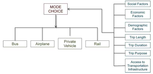
Figure 3-8. Visualization of Simple Multinomial Logit Model.
The mathematical form of the multinomial logit model is as follows. Suppose there are m total travel modes of interest (1, 2, 3, … M) and that there are k factors (1, 2, 3, …, K) that are being used to predict the probability of a particular mode choice. These k factors in general may include continuous, binomial, or categorical data. To construct the logits in the multinomial case, one of the modes is considered the reference level and all other logits are constructed relative to it. Any mode can be taken as the reference level since there is no inherent ordering to the modes. Here mode M is taken as the reference level. The probability of an individual i selecting a travel mode m, out of M number of total available modes, is represented as Pim. The relationship between this probability and the K factors is given by the following multinomial logistic regression model
where,
x1i, …, xki are the k number of factors of mode m for individual i;
β0m is the mode specific constant for mode m;
β1m, …, βkm are k number of coefficients of mode m which need to be estimated from the data;
M is the set of all available travelling modes; and
n is the number of individual/trip combinations in the dataset.
The above equation can be solved to yield the probability of an individual i selecting a travel mode m, out of M number of total available modes as
and for the reference category,
For this research, the model in Equation (1) was fitted separately to the three different trip purposes (business, personal business, and pleasure). The number of modes (M) was equal to four (personal vehicle, air, bus, and train) where personal vehicle was considered the base level. The predictive factors included in each model are summarized in Table 3-1.
The form of the discrete choice multinomial logit model used in this research is based on the assumption that the choice of mode is a function of the characteristics of the traveler and/or the trip. This is known as a generalized multinomial logit model or unconditional multinomial logit model. The NHTS neither collected data that characterize the different available mode choices (e.g., travel time or cost under each of the mode options) nor did it provide information about other alternative modes or the traveler’s reason for selecting a specific mode of travel over another mode. As such, a conditional multinomial logit model, a model where the choice of mode is a function of the characteristics of the respective modes themselves, could not be utilized without developing synthetic estimates for variables such as travel cost. This has been done in previous research (Ashiabor et al, 2007). The resources available to this research project did not allow for this type of data collection and use. Travel cost and other attributes not found in the NHTS are accounted for through economic and other proxies described in Section 3.2.
3.5.2 Model Estimation
The 2001 NHTS provides an analysis weight for each long-distance trip. The weight is defined at the person trip/travel period level. These weights reflect the selection probabilities and adjustments to account for nonresponse, undercoverage, and multiple telephones in a household. Point estimates of population parameters as well as coefficients of predictors are impacted by the value of the analysis weight for each observation. To obtain estimates that are minimally biased the analysis weight (WTPTPFIN) was used to weight the results.
Coefficients associated with each predictive factor were estimated using the maximum likelihood estimation technique in the SAS® (version 9.3) statistical software package. The SURVEYLOGISTIC procedure was used to take into account the complex nature of the 2001 NHTS sample design. This procedure was preferred over the CATMOD and PHREG procedures both of which can perform multinomial logistic regression but are based on the assumption that the sample is drawn from an infinite population by simple random sampling. If the sample is actually selected from a finite population using a complex design, these procedures generally do not calculate the estimates and their variances correctly. Namely, they fail to take into account the following characteristics of sample survey data that are present in the 2001 NHTS data and hence, generally underestimate the variance of point estimates and model coefficients:
- Unequal selection probabilities;
- Stratification;
- Clustering of observations; and
- Nonresponse and other adjustments.
The SURVEYLOGISTIC procedure fits linear logistic regression models while incorporating complex survey sample designs, including designs with stratification, clustering, and unequal weighting. In this research, the jackknife variance estimation method was used. The jackknife is a replication-based variance estimation method whereby subsamples of the original sample (replicate samples) are taken and the model coefficients are estimated for each replicate sample. The variability of the estimated model coefficients among the replicate samples is then used as a replication-based estimator of variance. Replicate weights calculated using the delete-one Jackknife method and provided on the 2001 NHTS website were used in the modeling.
Model coefficients for the predictor variables were estimated from the model. Logistic regression coefficients are difficult to interpret because they measure the effect that a change in an independent variable would have on the log odds of choosing a particular mode choice. As a result, the coefficient estimates in this analysis were transformed into marginal probability effects. Marginal probability effects are more intuitive in that they represent the effect that a change in the independent variable would have directly on the probability of choosing the mode choice. STATA (version 11) was used to calculate these marginal estimates as the SURVEYLOGISTIC procedure does not support this capability.
To assess the model fit, goodness of fit statistics such as the overall model chi-square, log-likelihood values, and pseudo- R2 values were examined. These statistics provided evidence of a good model fit (i.e. they have values close to 1). While multinomial logistic regression does compute these measures to estimate the strength of the relationship, these correlation measures alone do not provide sound evidence for determining and estimating the accuracy or errors associated with the model. Moreover, the overall model chi-square, log likelihood values, and pseudo- R2 values can become quite large for data with large weights and this results in the generalized R-square almost always being 1. Therefore, to assess the model’s predictive ability, the model was applied to the dataset of trips to determine its predictive ability. Aggregate mode shares were calculated by summing the calculated probabilities for each trip record. These were compared against the actual mode shares of the data set of trips in order to observe how well the model could replicate the observed mode shares.
3.6 Model Estimation Results
This section contains model estimation results for both the full mode-choice prediction models (Section 3.6.1) and the reduced mode-choice prediction models (Section 3.6.2). Results from the full model are presented to collectively assess the predictive ability of all variables identified in Section 3.2 for mode choice. These results identify those variables that are highly predictive of mode choice so that a general understanding of long-distance travel mode choice can be realized without the worry that some inputs are not readily available for future mode prediction. The reduced model can be used in a more practical sense to predict future mode choice within a transportation modeling framework as it contains only readily available input variables identified as having an influence on mode choice.
3.6.1 Full Prediction Models
Coefficient estimates and their standard errors for the multinomial logit models of travel mode choice are presented in Table 3-4, with one set of coefficient results for each travel purpose type. Separate model estimates are presented for each travel mode. Note that there are no coefficient estimates for the personal vehicle mode as that mode was the reference level. Thus, the logits for all other modes are constructed relative to it. Also for those categorical variables with more than two levels (income and race) one of the levels for each variable was used as the reference category and thus no coefficients were estimated. For income, estimates for all levels were made relative to the greater than $100,000 category while for race, estimates for all levels were made relative to white travelers. Coefficient estimates significant at the 1, 5, and 10 percent level of significance are noted with a ‘**’, ‘*’, and ‘+’, respectively.
| Business: Private Vehicle | Business: Air | Business: Bus | Business: Train | Pleasure: Private Vehicle | Pleasure: Air | Pleasure: Bus | Pleasure: Train | Personal Business: Private Vehicle | Personal Business: Air | Personal Business: Bus | Personal Business: Train | |
|---|---|---|---|---|---|---|---|---|---|---|---|---|
| Post 9/11 (d) | -0.3461 (0.2737) |
-0.5787 (0.9486) |
-1.3608* (0.6298) |
-0.2518 (0.2288) |
0.8113 (0.5605) |
0.1744 (0.7392) |
-0.5193 (0.5656) |
0.7281 (0.4754) |
-3.2055 (2.8332) |
|||
| Trip occurred on weekend (d) |
0.4426* (0.2009) |
-0.5726 (0.8082) |
1.7378* (0.6680) |
0.7664** (0.1476) |
0.1232 (0.3343) |
0.0515 (0.3950) |
0.9560** (0.3362) |
-0.5491 (0.4833) |
2.3317 (2.2458) |
|||
| Nights away on trip |
0.0510 (0.0525) |
-0.1893 (0.3612) |
-1.0593* (0.5286) |
-0.0197 (0.0155) |
-0.2212* (0.1068) |
0.0109 (0.0222) |
-0.0140 (0.0128) |
-0.1253+ (0.0686) |
-0.9871 (0.6754) |
|||
| Number of people on trip |
0.1130** (0.0402) |
0.2971** (0.0677) |
-0.0467 (0.2922) |
-0.0175 (0.0348) |
0.1838** (0.0194) |
0.1134 (0.1570) |
-0.0937 (0.1563) |
0.2711** (0.0576) |
0.1448 (0.1033) |
|||
| Respondent’s age |
-0.0020 (0.0086) |
0.0683+ (0.0365) |
0.0133 (0.0216) |
-0.0067 (0.0044) |
-0.0076 (0.0121) |
-0.0089 (0.0170) |
-0.0075 (0.0118) |
-0.0350+ (0.0207) |
-0.0088 (0.0388) |
|||
| Trip distance |
0.0054** (0.0007) |
0.0036 (0.0025) |
0.0036 (0.0026) |
0.0043** (0.0003) |
0.0014** (0.0005) |
0.0021** (0.0005) |
0.0049** (0.0006) |
0.0024** (0.0009) |
0.0031 (0.0021) |
|||
| Count of vehicles in HH |
-0.4201** (0.0975) |
0.0419 (0.1326) |
-0.0142 (0.2602) |
-0.1945* (0.0823) |
-0.2017 (0.1423) |
-0.6012 (0.3746) |
0.0005 (0.1306) |
-0.2473 (0.2898) |
-0.3821 (1.0886) |
|||
| Urban HH |
0.5276* (0.2560) |
0.3258 (1.0243) |
-0.4369 (0.8495) |
0.8068** (0.2750) |
-0.3751 (0.3639) |
0.2356 (0.8725) |
0.4905 (0.4459) |
-0.7594 (0.7307) |
-0.7856 (1.7244) |
|||
| Population per sq mile |
-0.0000 (0.0000) |
0.0000 (0.0001) |
0.0000 (0.0001) |
-0.0000 (0.0000) |
0.0000 (0.0000) |
-0.0000 (0.0000) |
0.0001 (0.0000) |
-0.0001 (0.0000) |
0.0000 (0.0001) |
|||
| Count of all bus depots in 25M radius |
-0.0118 (0.0625) |
-0.1071 (0.1715) |
-0.1948 (0.1694) |
-0.0109 (0.0455) |
-0.0543 (0.0770) |
0.0950 (0.1533) |
-0.0632 (0.1174) |
-0.2657* (0.1228) |
0.2986 (0.4052) |
|||
| Count of all airports in 25M radius |
0.3199** (0.1157) |
-0.1117 (0.5570) |
-0.1150 (0.3497) |
0.1221 (0.0862) |
-0.2026 (0.1630) |
-0.1826 (0.3672) |
-0.1406 (0.2679) |
0.9176** (0.1899) |
0.7236 (0.8637) |
|||
| Count of all Amtrak stations in 25M radius |
-0.0273 (0.0314) |
-0.0822 (0.1618) |
0.0336 (0.0717) |
0.0243 (0.0220) |
0.0087 (0.0663) |
-0.0356 (0.0915) |
-0.0405 (0.0744) |
0.0993 (0.1165) |
-0.1798 (0.3293) |
|||
| Count of all transit/subway/light/commuter rail stations in 25M radius |
-0.0019 (0.0012) |
0.0017 (0.0036) |
0.0017 (0.0032) |
0.0004 (0.0006) |
0.0002 (0.0013) |
0.0039 (0.0033) |
0.0002 (0.0024) |
0.0003 (0.0018) |
-0.0025 (0.0077) |
|||
| CPI Private Transport, seasonally adjusted |
-0.0338 (0.0403) |
-0.2557 (0.1906) |
-0.2005 (0.1462) |
-0.0663+ (0.0342) |
0.0888 (0.0675) |
-0.0205 (0.1106) |
-0.0105 (0.0815) |
0.1069 (0.0827) |
0.0294 (0.5872) |
|||
| CPI Public Transport, seasonally adjusted |
-0.0161 (0.0597) |
-0.1172 (0.2254) |
0.0669 (0.1722) |
0.0833 (0.0584) |
-0.1087 (0.0670) |
0.0057 (0.1574) |
0.0161 (0.1064) |
0.1254 (0.1942) |
-0.9336 (0.8419) |
|||
| RITA airline ticket price index |
0.0109 (0.0316) |
0.0541 (0.1609) |
0.0328 (0.0734) |
0.0012 (0.0268) |
0.0123 (0.0486) |
0.0676 (0.0817) |
-0.0194 (0.0603) |
0.0589 (0.0650) |
-0.4087 (0.3565) |
|||
| Weekly use of public/commercial transportation (d) |
0.7521** (0.2167) |
2.4052** (0.7928) |
3.4173** (0.8193) |
0.4212* (0.1727) |
1.4132** (0.2421) |
1.3816** (0.4469) |
0.2743 (0.4617) |
0.6062 (0.6275) |
1.8978+ (0.9929) |
|||
| Weekly web use (d) |
1.3580** (0.3729) |
-0.2750 (0.9399) |
0.1228 (0.8525) |
0.1543 (0.1534) |
0.3689 (0.2951) |
0.0758 (0.5304) |
0.4193 (0.4511) |
0.4555 (0.6058) |
2.7481* (1.2755) |
|||
| $0<=Income<=$30,000 (d) |
-2.1512** (0.5319) |
-1.4185 (2.9038) |
0.5590 (0.9606) |
-1.0238** (0.2806) |
0.7819* (0.3874) |
0.3160 (0.8443) |
-1.2558+ (0.7367) |
0.8275 (0.9144) |
-0.3230 (27.0395) |
|||
| $30,000<Income<=$60,000 (d) |
-2.3332** (0.3171) |
0.6971 (1.8419) |
-0.2128 (0.8065) |
-0.7273** (0.2357) |
0.4677 (0.3919) |
-0.0407 (0.7911) |
-0.9963* (0.4473) |
0.4815 (0.8650) |
-0.4246 (1.8705) |
|||
| $60,000<Income<=$100,000 (d) |
-0.6823** (0.1901) |
0.6674 (1.7838) |
-0.5281 (0.6104) |
-0.5683** (0.1883) |
0.4795 (0.4290) |
0.1507 (0.8674) |
-0.8241* (0.3880) |
0.9803 (0.7145) |
0.6000 (1.3690) |
|||
| $100,000<Income (d) | Omitted – Reference Category | Omitted – Reference Category | Omitted – Reference Category | Omitted – Reference Category | Omitted – Reference Category | Omitted – Reference Category | Omitted – Reference Category | Omitted – Reference Category | Omitted – Reference Category | Omitted – Reference Category | Omitted – Reference Category | Omitted – Reference Category |
| African-American (d) |
-0.2763 (0.4554) |
-0.8361 (1.5783) |
-0.3266 (1.1267) |
-0.1580 (0.3887) |
1.3575** (0.4414) |
-0.7992 (24.1714) |
-1.1674 (0.9106) |
0.0936 (0.6214) |
-25.5720** (6.0584) |
|||
| Asian (d) |
1.5184+ (0.9113) |
-28.4430 (28.7475) |
-1.3924 (30.7627) |
0.0668 (0.6076) |
-0.3040 (0.8522) |
-2.0277 (23.6137) |
-28.7018** (6.4247) |
0.8211 (1.2124) |
-28.5955** (10.4811) |
|||
| Hispanic (d) |
0.3891 (0.5068) |
-24.7044** (5.8215) |
-29.3618** (10.0109) |
-0.2779 (0.6820) |
-0.2395 (1.3593) |
-24.6207** (5.5158) |
-3.0742 (24.4496) |
-4.2341 (22.5459) |
-23.8825** (6.9829) |
|||
| Other (d) |
0.5121 (0.8494) |
-1.2343 (23.0448) |
1.1816 (31.5731) |
0.2508 (0.3891) |
-0.8336 (1.2065) |
1.3186 (0.8097) |
-1.3535 (24.8385) |
-0.4788 (1.9753) |
-27.8318** (7.6088) |
|||
| White (d) | Omitted – Reference Category | Omitted – Reference Category | Omitted – Reference Category | Omitted – Reference Category | Omitted – Reference Category | Omitted – Reference Category | Omitted – Reference Category | Omitted – Reference Category | Omitted – Reference Category | Omitted – Reference Category | Omitted – Reference Category | Omitted – Reference Category |
| Respondent is employed (d) | Omitted – Business trips were assumed to occur only for survey respondents who were employed | Omitted – Business trips were assumed to occur only for survey respondents who were employed | Omitted – Business trips were assumed to occur only for survey respondents who were employed |
0.1672 (0.1479) |
-0.7194** (0.2397) |
-0.2637 (0.4686) |
0.3540 (0.3494) |
-0.2628 (0.4162) |
-0.4557 (1.4084) |
|||
| Constant |
3.1080 (13.7928) |
47.0182 (50.0787) |
7.6112 (32.1389) |
-12.4997 (13.6170) |
3.3135 (21.9081) |
-10.8349 (41.3653) |
-4.1895 (27.7211) |
-53.9195 (35.6857) |
226.8973 (214.9397) |
Raw model coefficient results for maximum likelihood models can indicate statistical significance and the direction of an effect that is attributable to a certain variable, but do not give meaningful insight into the actual probabilistic changes attributable to specific variables. To show a more useful interpretation, coefficient estimates in this analysis were transformed into marginal probability effects. Marginal effects give the marginal probabilistic change in an outcome that is attributable to a given variable; for example, for a single unit of change in one variable (a marginal change), the marginal effect coefficient gives the increase or decrease in probability of observing an outcome due to that single unit change. As a more concrete example, consider the marginal effect coefficient associated with whether the trip occurred on a weekend. The marginal coefficient for personal vehicle travel (-0.0299) for business trips means that the probability of taking a personal vehicle decreases by almost three percent when the trip includes a weekend versus when it does not. Marginal effects are calculated conditional on all other model coefficients at the sample averages, which often make them more useful in predictive analyses than odds ratios, another type of transformation of maximum likelihood model results that does not condition on other model coefficients. The transformed model coefficients in their marginal effects form along with their standard errors (in parentheses) are shown below in Table 3-5.
| Business: Private Vehicle | Business: Air | Business: Bus | Business: Train | Pleasure: Private Vehicle | Pleasure: Air | Pleasure: Bus | Pleasure: Train | Personal Business: Private Vehicle | Personal Business: Air | Personal Business: Bus | Personal Business: Train | |
|---|---|---|---|---|---|---|---|---|---|---|---|---|
| Post 9/11 (d) |
0.0191 (0.0129) |
-0.0152 (0.0124) |
-0.0006 (0.0011) |
-0.0034 (0.0044) |
0.0007 (0.0071) |
-0.0066 (0.0059) |
0.0056 (0.0040) |
0.0003 (0.0013) |
0.0002 (0.0090) |
-0.0046 (0.0072) |
0.0044 (0.0057) |
|
| Trip occurred on weekend (d) |
-0.0299+ (0.0161) |
0.0222+ (0.0120) |
-0.0005 (0.0007) |
0.0082 (0.0100) |
-0.0222** (0.0048) |
0.0214** (0.0042) |
0.0007 (0.0023) |
-0.0080 (0.0135) |
0.0109 (0.0127) |
-0.0029 (0.0038) |
||
| Nights away on trip |
0.0001 (0.0031) |
0.0023 (0.0023) |
-0.0002 (0.0004) |
-0.0023 (0.0023) |
0.0019* (0.0008) |
-0.0005 (0.0004) |
-0.0015* (0.0007) |
0.0009 (0.0008) |
-0.0001 (0.0002) |
-0.0007 (0.0008) |
||
| Number of people on trip |
-0.0051* (0.0021) |
0.0049* (0.0019) |
0.0003 (0.0003) |
-0.0001 (0.0006) |
-0.0010 (0.0010) |
-0.0005 (0.0009) |
0.0013** (0.0002) |
0.0002 (0.0004) |
-0.0008 (0.0021) |
-0.0008 (0.0016) |
0.0016 (0.0015) |
|
| Respondent’s age |
-0.0000 (0.0004) |
-0.0001 (0.0004) |
0.0001 (0.0001) |
0.0002 (0.0001) |
-0.0002 (0.0001) |
-0.0001 (0.0001) |
0.0003 (0.0002) |
-0.0001 (0.0001) |
-0.0002 (0.0002) |
|||
| Trip distance |
-0.0002** (0.0000) |
0.0002** (0.0000) |
-0.0001** (0.0000) |
0.0001** (0.0000) |
0.0000* (0.0000) |
-0.0001 (0.0001) |
||||||
| Count of vehicles in HH |
0.0181** (0.0042) |
-0.0182** (0.0041) |
0.0001 (0.0001) |
0.0071** (0.0026) |
-0.0048* (0.0021) |
-0.0013 (0.0010) |
-0.0009 (0.0016) |
0.0014 (0.0020) |
-0.0015 (0.0019) |
|||
| Urban HH (d) |
-0.0199* (0.0097) |
0.0207* (0.0093) |
0.0003 (0.0010) |
-0.0011 (0.0023) |
-0.0144* (0.0064) |
0.0170** (0.0051) |
-0.0030 (0.0031) |
0.0003 (0.0014) |
0.0016 (0.0095) |
0.0039 (0.0059) |
-0.0054 (0.0073) |
|
| Population per sq mile | ||||||||||||
| Count of all bus depots in 25M radius |
0.0010 (0.0028) |
-0.0005 (0.0027) |
-0.0001 (0.0002) |
-0.0004 (0.0005) |
0.0005 (0.0015) |
-0.0003 (0.0011) |
-0.0004 (0.0005) |
0.0002 (0.0003) |
0.0021 (0.0020) |
-0.0005 (0.0012) |
-0.0016 (0.0018) |
|
| Count of all airports in 25M radius |
-0.0135** (0.0050) |
0.0139** (0.0046) |
-0.0001 (0.0005) |
-0.0003 (0.0008) |
-0.0014 (0.0030) |
0.0031 (0.0021) |
-0.0014 (0.0011) |
-0.0003 (0.0008) |
-0.0042 (0.0058) |
-0.0013 (0.0027) |
0.0054 (0.0055) |
|
| Count of all Amtrak stations in 25M radius |
0.0012 (0.0014) |
-0.0012 (0.0014) |
-0.0001 (0.0002) |
0.0001 (0.0002) |
-0.0006 (0.0007) |
0.0006 (0.0006) |
0.0001 (0.0005) |
-0.0001 (0.0002) |
-0.0002 (0.0012) |
-0.0004 (0.0008) |
0.0006 (0.0009) |
|
| Count of all transit/subway/light/commuter rail stations in 25M radius |
0.0001 (0.0001) |
-0.0001 (0.0001) |
||||||||||
| CPI Private Transport, seasonally adjusted |
0.0021 (0.0019) |
-0.0014 (0.0017) |
-0.0002 (0.0003) |
-0.0004 (0.0005) |
0.0011 (0.0010) |
-0.0017* (0.0008) |
0.0006 (0.0005) |
-0.0005 (0.0011) |
-0.0001 (0.0007) |
0.0006 (0.0009) |
||
| CPI Public Transport, seasonally adjusted |
0.0007 (0.0027) |
-0.0007 (0.0026) |
-0.0001 (0.0003) |
0.0001 (0.0004) |
-0.0014 (0.0016) |
0.0021 (0.0015) |
-0.0008 (0.0005) |
-0.0009 (0.0016) |
0.0001 (0.0009) |
0.0007 (0.0013) |
||
| RITA airline ticket price index |
-0.0006 (0.0014) |
0.0005 (0.0013) |
0.0001 (0.0002) |
0.0001 (0.0001) |
-0.0002 (0.0008) |
0.0001 (0.0003) |
0.0001 (0.0002) |
-0.0002 (0.0008) |
-0.0002 (0.0006) |
0.0003 (0.0006) |
||
| Weekly use of public/commercial transportation (d) |
-0.0795* (0.0389) |
0.0386* (0.0150) |
0.0061 (0.0074) |
0.0348 (0.0380) |
-0.0321** (0.0093) |
0.0116* (0.0056) |
0.0167** (0.0050) |
0.0038 (0.0054) |
-0.0071 (0.0111) |
0.0026 (0.0057) |
0.0046 (0.0082) |
|
| Weekly web use (d) |
-0.0451** (0.0100) |
0.0453** (0.0098) |
-0.0003 (0.0012) |
0.0002 (0.0017) |
-0.0061 (0.0044) |
0.0037 (0.0035) |
0.0023 (0.0018) |
0.0001 (0.0008) |
-0.0057 (0.0055) |
0.0033 (0.0047) |
0.0024 (0.0029) |
|
| $0<=Income<=$30,000 (d) |
0.0460** (0.0068) |
-0.0469** (0.0059) |
-0.0008 (0.0012) |
0.0017 (0.0040) |
0.0107 (0.0068) |
-0.0188** (0.0038) |
0.0075 (0.0048) |
0.0006 (0.0021) |
0.0013 (0.0149) |
-0.0079 (0.0098) |
0.0065 (0.0115) |
|
| $30,000<Income<=$60,000 (d) |
0.0743** (0.0104) |
-0.0750** (0.0101) |
0.0009 (0.0024) |
-0.0003 (0.0014) |
0.0133* (0.0066) |
-0.0168** (0.0051) |
0.0036 (0.0031) |
0.0043 (0.0113) |
-0.0075 (0.0095) |
0.0032 (0.0072) |
||
| $60,000<Income<=$100,000 (d) |
0.0280** (0.0087) |
-0.0277** (0.0077) |
0.0007 (0.0021) |
-0.0010 (0.0015) |
0.0091 (0.0061) |
-0.0131** (0.0039) |
0.0037 (0.0036) |
0.0003 (0.0015) |
-0.0010 (0.0111) |
-0.0063 (0.0076) |
0.0073 (0.0089) |
|
| $100,000<Income (d) | Omitted – Reference Category | Omitted – Reference Category | Omitted – Reference Category | Omitted – Reference Category | Omitted – Reference Category | Omitted – Reference Category | Omitted – Reference Category | Omitted – Reference Category | Omitted – Reference Category | Omitted – Reference Category | Omitted – Reference Category | Omitted – Reference Category |
| African-American (d) |
0.0118 (0.0165) |
-0.0107 (0.0155) |
-0.0006 (0.0010) |
-0.0006 (0.0020) |
-0.0129 (0.0189) |
-0.0041 (0.0086) |
0.0179+ (0.0106) |
-0.0009 (0.0179) |
0.0062 (0.0100) |
-0.0068 (0.0086) |
0.0006 (0.0041) |
|
| Asian (d) |
-0.1285 (0.1340) |
0.1315 (0.1329) |
-0.0013 (0.0012) |
-0.0017 (0.0144) |
0.0014 (0.0179) |
0.0018 (0.0163) |
-0.0018 (0.0044) |
-0.0014 (0.0057) |
0.0048 (0.0240) |
-0.0124 (0.0146) |
0.0075 (0.0184) |
|
| Hispanic (d) |
-0.0125 (0.0304) |
0.0204 (0.0303) |
-0.0022 (0.0020) |
-0.0057 (0.0058) |
0.0102 (0.0163) |
-0.0061 (0.0133) |
-0.0014 (0.0074) |
-0.0027 (0.0042) |
0.0161 (0.0136) |
-0.0092 (0.0134) |
-0.0069* (0.0033) |
|
| Other (d) |
-0.0314 (0.1928) |
0.0276 (0.0605) |
-0.0007 (0.0064) |
0.0045 (0.2053) |
-0.0073 (0.0165) |
0.0071 (0.0123) |
-0.0040 (0.0037) |
0.0042 (0.0086) |
0.0089 (0.0587) |
-0.0067 (0.0591) |
-0.0023 (0.0079) |
|
| White (d) | Omitted – Reference Category | Omitted – Reference Category | Omitted – Reference Category | Omitted – Reference Category | Omitted – Reference Category | Omitted – Reference Category | Omitted – Reference Category | Omitted – Reference Category | Omitted – Reference Category | Omitted – Reference Category | Omitted – Reference Category | Omitted – Reference Category |
| Respondent is employed (d) | Omitted – Business trips were assumed to occur only for survey respondents who were employed | Omitted – Business trips were assumed to occur only for survey respondents who were employed | Omitted – Business trips were assumed to occur only for survey respondents who were employed | Omitted – Business trips were assumed to occur only for survey respondents who were employed |
0.0024 (0.0045) |
0.0042 (0.0035) |
-0.0061* (0.0027) |
-0.0005 (0.0011) |
-0.0012 (0.0057) |
0.0029 (0.0044) |
-0.0017 (0.0033) |
Note that some coefficient estimates that displayed statistical significance are no longer significant at any level once transformed into marginal effects. This can be due to a variety of reasons, but generally indicates that an overall relationship and its direction can be observed in the data but the exact effect may be more uncertain due to variability. Note also that personal vehicle outcome marginal effects are included in Table 3-5; although the raw coefficient estimates for multinomial logit models must be calculated relative to a base outcome, marginal effects can be estimated for each individual outcome – this is another reason for using these estimates in analyses where predictive conclusions are necessary. Some marginal effects were extremely small in magnitude (less than 0.0001, or a 0.01 percent change) and were not statistically significant. These were excluded from Table 3-5 because their predictive effect is minimal and the practical interpretations of their marginal effects are not useful for any further analysis. As in Table 3-4, one category for each of the income and race factors was used as the reference category and thus no marginal effects were estimated. Marginal effects significant at the 1, 5, and 10 percent level of significance are noted with a ‘**’, ‘*’, and ‘+’, respectively.
The model results display some consistent patterns in both coefficient and marginal effects estimates. First, there are a much higher number of statistically significant relationships observed across trip purpose types for personal vehicle and air travel outcomes. This is not entirely unexpected given the earlier discussion of the much lower number of observations for bus and train travel outcomes. Second, characteristics of the survey respondents who were taking the trips tended to be more significant predictors of travel mode choice than the characteristics of the trips themselves. This indicates that people’s travel mode choices may be driven largely by fixed attributes that revolve around residence and demographics rather than consideration of the dynamic costs and benefits of different modes of travel. The marginal effects also suggest that respondents’ demand for different modes of travel is relatively decoupled from cost considerations such as the price of airfares or gasoline and that the preference set may be fairly inelastic in the short term – that is, not responsive to changes in price. This is difficult to state emphatically because the exact cost of each travel option for each trip is not known but the evidence leads to this conclusion based on the economic variables used in the model. Small marginal effects, which often include the value zero within the range of one standard deviation, for price indices indicate that respondents tended to be fixed in their travel mode preferences conditional on the fixed residence and demographic attributes.
Marginal effects for variables describing trip characteristics other than distance tended to have mixed effects for different travel mode outcomes. There was little evidence that the 9/11 terrorist attacks had a noticeable effect on travel mode choices, as no marginal effects were significant. This is especially noteworthy for air travel modes as it shows that perceptions of terrorism safety may not be major drivers of respondents’ choices. A weekend trip had a statistically significant marginal effect for personal vehicle and air travel for the two largest travel purpose types. There was a two to three percent decrease in the probability of taking a personal vehicle and a two percent increase in the probability of taking air travel if the trip included a weekend for business and pleasure travel. The number of persons on the trip also significantly impacted likelihoods of different mode choices; for business travel it corresponded to a 0.5 percent decrease in the chances of taking personal vehicle per person and a 0.5 percent increase in the chances of taking air travel while for pleasure travel it increased chances of taking bus travel by 0.13 percent per person. This is likely due to vehicle use efficiency reasons for business travel and the appeal of bus sightseeing tours for pleasure travel. Lastly, for pleasure travel, the number of nights away increased the probability of taking personal vehicles by 0.19 percent a night and decreased the probability of taking bus travel by 0.15 percent a night. The route travel distance was highly significant for both business and pleasure travel, and will be discussed separately.
Variables describing characteristics about respondents’ place of residence also displayed mixed results. Classification of a residence as a “rural” or “urban” area was a significant predictor for personal vehicle and air mode choices, and corresponded to approximately a two percent increased chance of taking air travel for business and a 1.97 percent increased chance of taking air travel for pleasure with corresponding decreases in probability for taking personal vehicles for urban areas as compared to rural areas. Conditional on urban or rural classification, population density did not appear to have any significant effect on travel mode choice. Available transportation infrastructure only appeared to be influential for business travel; the number of airports in a 25 mile radius increased the chances of taking air travel by 1.39 percent per airport. The accessibility or airports within driving or public transit distance seems to be a primary driver of choosing this mode for work travel, but does not appear to matter for other types of travel. This could again be related to time and efficiency constraints involved with business travel that are not present for other types. Other existing transportation infrastructure did not appear to play a significant role in travel choice, but this could also be a product of large numbers of observations in the data set that chose personal vehicle as the primary mode of transport and thus do not display any preferences towards certain types of existing networks.
Respondent’s demographic and behavioral variables were the most consistently significant predictors of travel choice for business and pleasure travel. Familiarity with public/commercial transportation systems through frequent usage resulted in a large decrease in the likelihood of taking personal vehicles for business travel (eight percent) as well as a smaller but still significant decrease in the likelihood of taking personal vehicles for pleasure travel (three percent). Interestingly, high public/commercial transportation use was highly statistically significant for predicting increases in the use of air travel (four percent for business, 1.2 percent for pleasure). This seems to indicate that a major factor in using air travel revolves around comfort with using the public transit system as an intermediate mode to get to or from an airport. For business travel, frequent web use also increased chances of taking air travel by about 4.5 percent; this result, as well as a corresponding decrease in chances of taking personal vehicles, was statistically significant at the 1 percent level. Past studies have cited familiarity with using online travel reservations as a potential predictor of demand for air travel, and this seems to be borne out by the model results (Civil Aviation Authority, 2005; Morrison et al, 2001). Income was also a strong predictor of travel mode choice for both business and pleasure travel. Relative to the reference category of income greater than $100,000 per year, the three lower income brackets were more likely to take personal vehicles and less likely to take air travel. The lower likelihood of air travel as income decreases shows the stronger statistical significance trend, and this reinforces the hypothesis that fixed attributes like income are much stronger determinants of travel mode. The marginal effects show that a household income that is unable to support the higher cost of air travel appears to display preferences towards personal vehicles based solely on income and not the price of airline tickets. It is possible that the price threshold for air travel faced by respondents during the survey period is high enough that consumers did not display any price sensitivity, but airline prices were relatively low during this period and displayed a reasonable range of variability during the period after 9/11. Overall, income and behavioral variables seemed to display the highest statistical significance in model results.
One of the most consistently significant variables in the model was route distance of a trip from origin to destination (measured in miles). This result reflects expected respondent preferences for transportation mode choice that can be observed in the larger U.S. population of travelers – longer trips place a higher inconvenience burden on personal vehicle travel and make other modes of travel, particularly air travel, more desirable. This is due to the physical, time, and financial burdens of traveling in a personal vehicle over increasingly large distances, and there is an expected “break even” point at which the desirability of personal vehicle travel begins to be outweighed by the convenience of other modes. The marginal effects coefficients listed in Table 3-5 give the marginal changes in probability of choosing each mode per additional mile traveled. On a per mile basis this is not a practical result to use in analysis of travel behavior since there might be very small overall marginal probability changes observed for short distance trips. In order to better observe the overall relationship between route distance and travel mode choice, Figures 3-9 through 3-11 display the trend in predicted probabilities the model outputs for travel mode choice for respondent observations at different route distances. The overall trend is estimated directly from the NHTS dataset using a nonparametric polynomial smoothing function to produce probability distributions that approximate the continuous change in predicted probabilities of mode choice over the range of trip route distances. This smoothing function gives a more concise picture of the significant relationships present in the data than a standard scatter plot graph.
Note that the graphs display probabilities of taking a certain mode of travel on the vertical axis, and thus the “break even” point for this representation shows a route distance at which the predicted probability of taking a private vehicle is approximately equal to the predicted probability of taking air travel. The predicted probabilities for each mode choice at a given trip distance shown in the figures represents a smoothed average across all the trips in the NHTS file at that distance. For example, the probability of taking private vehicle or air travel is each about 50 percent at about 700 miles for business travel (a small percentage of travelers choose train or bus). For some NHTS trips around 700 miles, the probability of taking a private vehicle for the given trip is greater than that of air travel (e.g., 70 percent for private vehicle, 20 percent for air, and 10 percent for bus/train) while for other trips around that distance the probability of taking air travel for the given trip is greater than that of a private vehicle (30 percent for private vehicle, 60 percent for air, and 10 percent for bus/train). The differences in predicted probabilities for trips are a result of the values for other predictors in the model. The data values used in Figures 3-9 through 3-11 show the smoothed mean predicted probabilities at a given distance.
The coast-to-coast driving distance in the main body of the U.S. is around 3,000 miles, so this is used as the upper bound of the figures (note that there are some outlier observations with route distances higher than 3,000 miles).
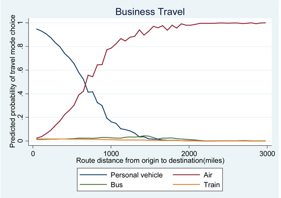
Figure 3-9. Fitted Polynomial Trend of Route Distance vs. Predicted Travel Mode Choice – Business Travel.
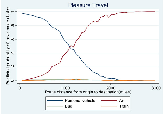
Figure 3-10. Fitted Polynomial Trend of Route Distance vs. Predicted Travel Mode Choice – Pleasure Travel.
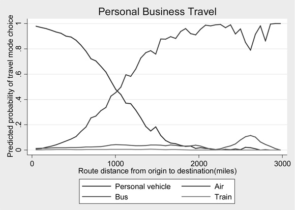
Figure 3-11. Fitted Polynomial Trend of Route Distance vs. Predicted Travel Mode Choice – Personal Business Travel.
The above figures show several clear trends. First, the probability of choosing to travel in a personal vehicle decreases exponentially with travel distance. Second, the probability of choosing air travel increases exponentially with travel distance. Last, there is a limited range of “break even” points across travel purpose types where the probability of taking air travel begins to exceed the probability of taking a personal vehicle. For business travel, this point occurs around 700 miles and is the lowest of all three travel modes. This is consistent with the need for efficient, short travel periods to conduct business with a lower upper distance tolerance for personal vehicle use that reaches time and convenience constraints more quickly. Pleasure trips have a much higher tolerance for personal vehicle use, with a “break even” point around 1,100 miles where air travel becomes more likely. This fits with more relaxed constraints surrounding pleasure travel, where the desirability of personal vehicles can remain higher over longer distances as part of sightseeing road trips. Personal business travel displays a trend that is between the other two types of travel, and also shows some signs of limited data issues due to the large swings in predicted probabilities at high route distances. Overall, bus and train travel modes do not display high predicted probabilities, and other than a few small increases at higher route distances do not display any significant trends.
The graph for personal business travel displays a noticeable increase in predicted probabilities of taking bus travel at route distances around 2,700 miles. This is due to a group of personal business travel observations in the dataset who all appear to have taken a group trip by bus at this distance, giving more weight to predicted probabilities of this mode and resulting in a corresponding decrease in the probability of taking air travel (the overwhelmingly predominant predicted mode at surrounding trip distances). While this increase is visible in the overall shape of the probability distribution for bus travel, note that the highest level of predicted probability is only about a 10 percent likelihood of taking bus travel which is still relatively small compared to the 80 percent likelihood of taking air travel at this distance. Thus this likely an artifact of the group of observations in the NHTS data at this distance as opposed to a predictive trend.
3.6.2 Reduced Prediction Models
Coefficient estimates and their standard errors for the reduced multinomial logit models of travel mode choice are presented in Table 3-6, with one set of coefficient results for each travel purpose type. Separate model estimates are presented for each travel mode. Note that there are no coefficient estimates for the personal vehicle mode as that mode was the reference level. Thus, the logits for all other modes are constructed relative to it. Also for the categorical variable income that has more than two levels, the greater than $100,000 category was used as the reference category and thus no coefficients were estimated. Estimates for all other levels were made relative to the greater than $100,000 category. Coefficient estimates significant at the 1, 5, and 10 percent level of significance are noted with a ‘**’, ‘*’, and ‘+’, respectively.
The reduced model coefficients indicate that many of the relationships observed in the fully specified model are preserved for the smaller subset of variables. Income categorical variables remained statistically significant as predictors of increased use of air travel at the 1 percent and 5 percent levels. Route distance also remained a significant determinant for the choice of using air travel relative to private vehicles. In contrast to the fully specified model, the number of people on the trip was a significant predictor for taking a bus, with larger numbers of people indicating increased probabilities of bus use across trip purposes at the 1 percent level.
Marginal effects were calculated for the reduced form model in the same way as the fully specified model, and are presented in Table 3-7. Some marginal effects were extremely small in magnitude (less than 0.0001, or a 0.01 percent change) and were not statistically significant. These were excluded from Table 3-7 because their predictive effect is minimal and the practical interpretations of their marginal effects are not useful for any further analysis. As in Table 3-6, one category for the income factor was used as the reference category and thus no marginal effects were estimated. Marginal effects significant at the 1, 5, and 10 percent level of significance are noted with a ‘**’, ‘*’, and ‘+’, respectively.
Many marginal effects retained similar significance and magnitude levels to the fully specified marginal effects with several exceptions. Despite the fact that the marginal effect for number of persons remained a significant factor for increased probabilities of bus usage for long distance trips, the marginal effect per additional trip person was relatively small meaning that a sufficiently large group of travelers would be needed to cause a noticeable shift in predictive probability. Income categorical variables all had increased marginal effect magnitudes in the reduced form model in addition to retaining their predictive significance. Relative to household incomes of greater than $100,000 per year, incomes of $60,000 to $100,000, $30,000 to $60,000, and less than $30,000 per year had 3.56 percent, 9.46 percent, and 5.91 percent lower chances of taking air travel for business travel, respectively. These decreased probabilities corresponded with similarly significant increases in the likelihood of taking a private vehicle relative to incomes over $100,000 per year. The same patterns for income are observed for pleasure and personal business trips although the marginal effects are less. Interestingly, for business travel only there was a statistically significant increase in the probability of taking private vehicles after 9/11.
| Business: Private Vehicle | Business: Air | Business: Bus | Business: Train | Pleasure: Private Vehicle | Pleasure: Air | Pleasure: Bus | Pleasure: Train | Personal Business: Private Vehicle | Personal Business: Air | Personal Business: Bus | Personal Business: Train | |
|---|---|---|---|---|---|---|---|---|---|---|---|---|
| Post 9/11 (d) |
-0.3531 (0.2541) |
-0.5725 (0.9464) |
-1.0829+ (0.5920) |
-0.1737 (0.2224) |
0.7769 (0.5260) |
0.2369 (0.6768) |
-0.5377 (0.5250) |
0.5793 (0.4608) |
-2.6685+ (1.3447) |
|||
| Number of people on trip |
0.1110** (0.0361) |
0.2605** (0.0607) |
-0.1512 (0.2728) |
-0.0310 (0.0372) |
0.1829** (0.0180) |
0.1088 (0.1628) |
-0.0705 (0.1386) |
0.2669** (0.0492) |
0.0982 (0.1006) |
|||
| Respondent’s age |
-0.0072 (0.0095) |
0.0657* (0.0330) |
0.0105 (0.0164) |
-0.0099* (0.0043) |
-0.0148 (0.0118) |
-0.0054 (0.0165) |
-0.0104 (0.0104) |
-0.0318+ (0.0189) |
-0.0147 (0.0287) |
|||
| Trip distance |
0.0058** (0.0006) |
0.0034+ (0.0019) |
0.0023 (0.0018) |
0.0040** (0.0002) |
0.0004 (0.0003) |
0.0021** (0.0005) |
0.0045** (0.0005) |
0.0018* (0.0008) |
0.0016 (0.0019) |
|||
| Count of vehicles in HH |
-0.4384** (0.0956) |
-0.0979 (0.1592) |
-0.2043 (0.2367) |
-0.2318** (0.0788) |
-0.2373 (0.1482) |
-0.7529+ (0.3842) |
-0.1222 (0.1342) |
-0.3283 (0.2358) |
-0.3332 (0.8535) |
|||
| Urban HH (d) |
0.6408* (0.2691) |
0.2312 (1.0199) |
-0.2282 (0.5998) |
0.7808** (0.2579) |
-0.3105 (0.3549) |
0.0353 (0.9082) |
0.6458 (0.4284) |
-0.8227 (0.6469) |
-0.3068 (1.5105) |
|||
| Population per sq mile |
-0.0000 (0.0000) |
0.0001 (0.0000) |
0.0001 (0.0001) |
-0.0000 (0.0000) |
0.0000 (0.0000) |
0.0000 (0.0000) |
0.0000 (0.0000) |
-0.0000 (0.0000) |
0.0001 (0.0001) |
|||
| Count of all bus depots in 25M radius |
0.0007 (0.0650) |
0.0079 (0.2565) |
-0.0728 (0.1280) |
-0.0139 (0.0431) |
-0.0176 (0.0723) |
-0.0120 (0.1224) |
-0.1146 (0.1274) |
-0.2510+ (0.1422) |
0.2232 (0.3528) |
|||
| Count of all airports in 25M radius |
0.1905+ (0.1043) |
-0.2012 (0.5653) |
0.0318 (0.2121) |
0.1616* (0.0772) |
-0.1873 (0.1572) |
0.2414 (0.2138) |
-0.0377 (0.2053) |
0.8451** (0.1712) |
0.4085 (0.4573) |
|||
| Count of all Amtrak stations in 25M radius |
-0.0165 (0.0315) |
-0.0436 (0.1364) |
0.0393 (0.0639) |
0.0308 (0.0212) |
0.0282 (0.0543) |
0.0197 (0.0757) |
-0.0331 (0.0887) |
0.0797 (0.1178) |
-0.1282 (0.2121) |
|||
| CPI Private Transport, seasonally adjusted |
-0.0359 (0.0370) |
-0.2365 (0.1753) |
-0.1489 (0.1321) |
-0.0576+ (0.0337) |
0.0707 (0.0620) |
-0.0052 (0.1025) |
-0.0184 (0.0739) |
0.0734 (0.0963) |
0.0004 (0.3137) |
|||
| CPI Public Transport, seasonally adjusted |
-0.0274 (0.0564) |
-0.1239 (0.2246) |
0.0592 (0.1408) |
0.0726 (0.0566) |
-0.1279+ (0.0713) |
0.0021 (0.1488) |
0.0269 (0.1141) |
0.0997 (0.1681) |
-0.7717+ (0.4309) |
|||
| RITA airline ticket price index |
0.0150 (0.0331) |
0.0338 (0.1630) |
0.0113 (0.0702) |
0.0084 (0.0267) |
0.0206 (0.0468) |
0.0593 (0.0780) |
-0.0248 (0.0594) |
0.0397 (0.0636) |
-0.2597 (0.1709) |
|||
| $0<=Income<=$30,000 (d) |
-2.2477** (0.5391) |
-1.3403 (2.1476) |
-0.0840 (0.7611) |
-1.1929** (0.2741) |
0.9018* (0.3481) |
0.0421 (0.7595) |
-1.5568* (0.6870) |
0.8899 (0.7500) |
-0.7114 (22.5901) |
|||
| $30,000<Income<=$60,000 (d) |
-2.4231** (0.3107) |
0.1595 (1.6071) |
-0.6127 (0.6879) |
-0.8548** (0.2303) |
0.5094 (0.3653) |
-0.2554 (0.7445) |
-1.3163** (0.4475) |
0.6325 (0.8326) |
-1.3072 (2.2160) |
|||
| $60,000<Income<=$100,000 (d) |
-0.7265** (0.2001) |
0.5673 (1.6429) |
-0.7161 (0.5725) |
-0.6306** (0.1855) |
0.4996 (0.4151) |
0.1149 (0.8629) |
-1.0345* (0.4317) |
1.0823 (0.6641) |
0.1292 (2.1829) |
|||
| $100,000<Income (d) | Omitted – Reference Category | Omitted – Reference Category | Omitted – Reference Category | Omitted – Reference Category | Omitted – Reference Category | Omitted – Reference Category | Omitted – Reference Category | Omitted – Reference Category | Omitted – Reference Category | Omitted – Reference Category | Omitted – Reference Category | Omitted – Reference Category |
| Respondent is employed (d) | Omitted – Business trips were assumed to occur only for survey respondents who were employed | Omitted – Business trips were assumed to occur only for survey respondents who were employed | Omitted – Business trips were assumed to occur only for survey respondents who were employed |
0.3009+ (0.1556) |
-0.7529** (0.2293) |
-0.2560 (0.4560) |
0.5761 (0.3616) |
-0.1892 (0.3994) |
-0.3480 (0.8966) |
|||
| Constant |
7.0166 (13.1780) |
48.6000 (50.6280) |
5.4695 (24.6072) |
-11.6122 (13.0819) |
9.9690 (22.2701) |
-10.9894 (39.9300) |
-3.6399 (27.4661) |
-41.0353 (29.0254) |
184.8157+ (108.0689) |
| Business: Private Vehicle | Business: Air | Business: Bus | Business: Train | Pleasure: Private Vehicle | Pleasure: Air | Pleasure: Bus | Pleasure: Train | Personal Business: Private Vehicle | Personal Business: Air | Personal Business: Bus | Personal Business: Train | |
|---|---|---|---|---|---|---|---|---|---|---|---|---|
| Post 9/11 (d) |
0.0431* (0.0211) |
-0.0176 (0.0143) |
-0.0025 (0.0047) |
-0.0229 (0.0177) |
-0.0023 (0.0077) |
-0.0051 (0.0063) |
0.0066 (0.0045) |
0.0008 (0.0021) |
0.0070 (0.0150) |
-0.0094 (0.0094) |
0.0046 (0.0040) |
-0.0022 (0.0106) |
| Number of people on trip |
-0.0041 (0.0057) |
0.0060** (0.0020) |
0.0012 (0.0008) |
-0.0031 (0.0054) |
-0.0009 (0.0010) |
0.0016** (0.0002) |
0.0004 (0.0005) |
-0.0009 (0.0022) |
-0.0012 (0.0022) |
0.0021** (0.0007) |
0.0001 (0.0003) |
|
| Respondent’s age |
-0.0001 (0.0007) |
-0.0004 (0.0005) |
0.0003 (0.0002) |
0.0002 (0.0003) |
0.0004* (0.0002) |
-0.0003* (0.0001) |
-0.0001 (0.0001) |
0.0004+ (0.0002) |
-0.0002 (0.0002) |
-0.0002* (0.0001) |
||
| Trip distance |
-0.0004** (0.0001) |
0.0003** (0.0000) |
-0.0001** (0.0000) |
0.0001** (0.0000) |
0.0000+ (0.0000) |
-0.0001** (0.0000) |
0.0001** (0.0000) |
|||||
| Count of vehicles in HH |
0.0269** (0.0070) |
-0.0231** (0.0050) |
-0.0003 (0.0008) |
-0.0035 (0.0042) |
0.0107** (0.0027) |
-0.0063** (0.0022) |
-0.0019 (0.0013) |
-0.0024* (0.0011) |
0.0048 (0.0031) |
-0.0020 (0.0023) |
-0.0025 (0.0019) |
-0.0002 (0.0010) |
| Urban HH (d) |
-0.0260 (0.0191) |
0.0305** (0.0112) |
0.0009 (0.0046) |
-0.0054 (0.0129) |
-0.0153* (0.0073) |
0.0183** (0.0052) |
-0.0031 (0.0035) |
0.0001 (0.0029) |
-0.0018 (0.0097) |
0.0099 (0.0063) |
-0.0079 (0.0079) |
-0.0002 (0.0015) |
| Population per sq mile | ||||||||||||
| Count of all bus depots in 25M radius |
0.0013 (0.0045) |
0.0001 (0.0034) |
-0.0014 (0.0024) |
0.0006 (0.0016) |
-0.0004 (0.0012) |
-0.0001 (0.0006) |
-0.0000 (0.0004) |
0.0037 (0.0026) |
-0.0019 (0.0021) |
-0.0019 (0.0014) |
0.0001 (0.0008) |
|
| Count of all airports in 25M radius |
-0.0096 (0.0088) |
0.0102+ (0.0051) |
-0.0010 (0.0030) |
0.0004 (0.0041) |
-0.0037 (0.0027) |
0.0045* (0.0021) |
-0.0016 (0.0014) |
0.0008 (0.0006) |
-0.0060 (0.0041) |
-0.0008 (0.0035) |
0.0065** (0.0022) |
0.0002 (0.0011) |
| Count of all Amtrak stations in 25M radius |
0.0003 (0.0022) |
-0.0009 (0.0017) |
-0.0002 (0.0007) |
0.0008 (0.0012) |
-0.0011 (0.0008) |
0.0009 (0.0006) |
0.0002 (0.0005) |
0.0001 (0.0003) |
-0.0006 (0.0015) |
0.0006 (0.0010) |
-0.0001 (0.0004) |
|
| CPI Private Transport, seasonally adjusted |
0.0056 (0.0035) |
-0.0017 (0.0019) |
-0.0011 (0.0009) |
-0.0028 (0.0026) |
0.0010 (0.0012) |
-0.0016+ (0.0009) |
0.0006 (0.0005) |
-0.0002 (0.0015) |
-0.0003 (0.0013) |
0.0006 (0.0009) |
||
| CPI Public Transport, seasonally adjusted |
0.0009 (0.0042) |
-0.0015 (0.0030) |
-0.0006 (0.0013) |
0.0012 (0.0027) |
-0.0010 (0.0017) |
0.0021 (0.0016) |
-0.0011+ (0.0007) |
-0.0007 (0.0033) |
0.0005 (0.0020) |
0.0008 (0.0012) |
-0.0005 (0.0025) |
|
| RITA airline ticket price index |
-0.0011 (0.0024) |
0.0008 (0.0017) |
0.0002 (0.0007) |
0.0002 (0.0013) |
-0.0006 (0.0009) |
0.0002 (0.0007) |
0.0002 (0.0004) |
0.0002 (0.0002) |
0.0003 (0.0014) |
-0.0004 (0.0010) |
0.0003 (0.0005) |
-0.0002 (0.0009) |
| $0<=Income<=$30,000 (d) |
0.0631** (0.0155) |
-0.0591** (0.0067) |
-0.0037 (0.0037) |
-0.0003 (0.0145) |
0.0117 (0.0081) |
-0.0232** (0.0035) |
0.0114+ (0.0059) |
0.0002 (0.0025) |
0.0093 (0.0144) |
-0.0185** (0.0062) |
0.0095 (0.0103) |
-0.0004 (0.0078) |
| $30,000<Income<=$60,000 (d) |
0.1021** (0.0175) |
-0.0946** (0.0115) |
0.0013 (0.0081) |
-0.0088 (0.0100) |
0.0175* (0.0078) |
-0.0217** (0.0052) |
0.0050 (0.0036) |
-0.0007 (0.0025) |
0.0143 (0.0119) |
-0.0193** (0.0070) |
0.0057 (0.0083) |
-0.0007 (0.0035) |
| $60,000<Income<=$100,000 (d) |
0.0448* (0.0171) |
-0.0356** (0.0096) |
0.0031 (0.0097) |
-0.0123 (0.0096) |
0.0107 (0.0072) |
-0.0160** (0.0042) |
0.0049 (0.0043) |
0.0004 (0.0028) |
0.0044 (0.0103) |
-0.0154* (0.0062) |
0.0109 (0.0079) |
0.0001 (0.0014) |
| $100,000<Income (d) | Omitted – Reference Category | Omitted – Reference Category | Omitted – Reference Category | Omitted – Reference Category | Omitted – Reference Category | Omitted – Reference Category | Omitted – Reference Category | Omitted – Reference Category | Omitted – Reference Category | Omitted – Reference Category | Omitted – Reference Category | Omitted – Reference Category |
| Respondent is employed (d) | Omitted – Business trips were assumed to occur only for survey respondents who were employed | Omitted – Business trips were assumed to occur only for survey respondents who were employed | Omitted – Business trips were assumed to occur only for survey respondents who were employed | Omitted – Business trips were assumed to occur only for survey respondents who were employed |
0.0010 (0.0051) |
0.0080* (0.0038) |
-0.0081* (0.0032) |
-0.0009 (0.0019) |
-0.0072 (0.0066) |
0.0090 (0.0055) |
-0.0016 (0.0035) |
-0.0002 (0.0016) |
3.6.3 Model Limitations
One assumption of the multinomial logit model is that the model error terms are independent and identically distributed. As a result, when the multinomial logit model is used to model choices, it relies on the assumption of independence of irrelevant alternatives (IIA) which is not always desirable. Ben-Akiva and Lerman (1985) give the definition as “the ratio of the chosen probabilities of any two alternatives is entirely unaffected by the systematic utilities of any other alternatives.” They continue on to show that IIA can produce imprecise estimates when a new mode with similar characteristics is introduced into the mode choice set. As such, more complicated models such as the nested logit model or mixed logit model are sometimes used as an extension of the multinomial logit model to capture the correlation of alternatives when alternatives are not independent. Despite this shortcoming, this research utilizes the multinomial logit model. This was done primarily because of the limitations imposed by the statistical software SAS. As mentioned previously, the NHTS utilizes a complicated sampling design that involves a large amount of clustering (i.e., multiple members of a household are surveyed regarding their long-distance trips). To ensure that the effect of this clustering, as well as other survey issues such as nonresponse, unequal selection probabilities, and stratification are taken into account when calculating variances for model estimates, the SURVEYLOGISTIC procedure was used. One limitation to this procedure is that it is not designed to accommodate nested or mixed logit models. SAS can handle such models but only with other procedures that are in turn not equipped to deal with complicated survey design data. Given the amount of clustering, the research team believed it more important to account for the survey design in the analysis rather than focus on a more complicated model that might relax the IIA. FHWA requested the models be developed in SAS. There may be alternative software packages that could fit more complicated models while accounting for the complicated survey design. However, this was not explored because the resources available to this research did not allow for further investigation and FHWA preferred the use of SAS for model development in this task order. This is an area for further research.
3.7 Discussion
This report presents a detailed discussion of the mathematical models and inputs to the models used to estimate mode choice for long-distance passenger travel. The report examines the effects that the traveler (in terms of their socioeconomic, demographic, and behavioral attributes), the trip (in terms of distance, purpose, length, and traveling party size), the availability of transportation infrastructure, and land-use characteristics has on the selection of travel mode for long-distance travel as measured by a generalized multinomial logit model. Major findings from this research are as follows:
- Summary statistic and model results provide evidence that mode choice varies by trip purpose and that separate models are warranted;
- There were a much greater number of factors found to significantly influence mode choice observed across trip purpose types for personal vehicle and air travel outcomes than bus and train outcomes. This is due, in part, to the low frequency of bus and train trips in the NHTS;
- Characteristics of the survey respondents who were taking the trips tended to be more significant predictors of travel mode choice than the characteristics of the trips themselves. This indicates that people’s travel mode choices may be driven largely by fixed attributes that revolve around residence and demographics rather than consideration of the dynamic costs and benefits of different modes of travel;
- The results suggest that respondents’ demand for different modes of travel may be relatively decoupled from cost considerations such as the price of airfares or gasoline and that the preference set may be fairly inelastic in the short run – that is, not responsive to changes in price;
- Available transportation infrastructure only appeared to be influential for business travel;
- Respondent’s demographic and behavioral variables were the most consistently significant predictors of travel choice for business and pleasure travel;
- One of the most consistently significant variables in predicting mode choice was route distance of a trip from origin to destination. The probability of choosing to travel in a personal vehicle decreases exponentially with travel distance while the probability of choosing air travel increases exponentially with travel distance; and
- The model predicts very well for the personal vehicle and air modes but loses some predictive power for the bus and train modes. The relative lack of predictive power for bus and train modes indicate that the survey data may not be sufficient to accurately assess some outcomes and that alternative sampling techniques should be explored in future national travel surveys that provide more data for bus and train trips.
A more thorough assessment of the model’s strengths and predictive power is presented in the following section. It will also describe some of the model limitations and suggestions for further research that could overcome these limitations.