U.S. Department of Transportation
Federal Highway Administration
1200 New Jersey Avenue, SE
Washington, DC 20590
202-366-4000

July, 2023
U.S. Department of Transportation
John A. Volpe National Transportation Systems Center
Don Pickrell
David Pace
Jacob Wishart
Claire Roycroft
Notice
This document is disseminated under the sponsorship of the Department of Transportation in the interest of information exchange. The United States Government assumes no liability for the contents or use thereof.
The United States Government does not endorse products or manufacturers. Trade or manufacturers’ names appear herein solely because they are considered essential to the objective of this report.
Figure 1. Licensed Drivers as a Percent of Driving-Age Population (1960-2021)
Figure 2. Light-Duty Vehicle Miles Traveled (Total and Per Capita, 1966-2021)
Figure 3. Truck VMT as a Percent of Total VMT (1966-2021)
Figure 4. Light-Duty VMT per Capita and Real Personal Disposable Income per Capita, Index 1966=1 (1966-2021)
Table 1. Alternative Variables Tested in Modeling Procedures
Table 2. S&P Global Baseline Long-Term Economic Forecasts: Spring 2023
Table 3. Explanatory Variables Included in Light-Duty VMT Forecasting Model
Table 4. Explanatory Variables Included in Combination Truck VMT Forecasting Model
Table 5. Explanatory Variables Included in Single-Unit Truck VMT Forecasting Model
This document details the process that the Volpe National Transportation Systems Center (Volpe) used to develop travel forecasting models for the Federal Highway Administration (FHWA). These models enable FHWA to forecast future changes in the use of passenger and freight vehicles (as measured by the number of vehicle-miles traveled, or VMT) that are likely to occur in response to predicted changes in future economic conditions and demographic trends. Forecasts of VMT developed using these models will inform and support the development of future transportation plans and policies by the Federal government and other transportation policy makers.
The FHWA VMT forecasting models provide forecasts of VMT for the entire U.S., disaggregated into three vehicle type categories defined by FHWA: light-duty passenger vehicles, including automobiles and light-duty trucks (FHWA Vehicle Classes 2 and 3); single-unit trucks (FHWA Vehicle Classes 5, 6, and 7); and combination trucks (FHWA Vehicle Classes 8 through 13).1
The FHWA VMT forecasting models were developed using widely employed and well-documented statistical and econometric techniques to estimate the influence of underlying economic and demographic factors on passenger and commercial vehicle use. Forecasts of these underlying demographic trends and economic factors are then used in conjunction with the models’ individual equations to develop forecasts of future VMT growth.
The sections that follow describe the model development process, including the specification and econometric estimation of the equations that comprise the final set of VMT forecasting models. The first section discusses the economic theory of travel demand, which provided the basis for identifying and selecting appropriate economic and demographic variables—those likely to influence the demand for vehicle trips—for testing and inclusion in the forecasting models.
The second section details the methodology employed in developing the forecasting equations and selecting the most reliable versions. It describes the statistical tests and criteria used to ensure that the selected equations combine historical explanatory power with accurate forecasting performance.
Subsequent sections of the report provide details of the specific models themselves. These sections offer further insight into the key influences on VMT incorporated in each individual equation.
Details of the VMT forecasts are available from FHWA by contacting:
Clayton Clark
FHWA, Room E83-420
U.S. Department of Transportation
1200 New Jersey Avenue, SE.
Washington, DC 20590
202-366-5053
Vehicle travel is a derived demand, meaning that a trip taken in either a passenger or commercial vehicle is typically a means to transport passengers or freight from some initial location to a desired geographic destination. Changes in the demand for motor vehicle travel arise from household members’ choices about how frequently and where to participate in away-from-home activities such as working, attending school, shopping, or recreation, and from producers’ decisions about facility locations and their output levels, sources of raw materials, and destinations for finished products. Generating predictions of how the amount of travel will change in the future thus requires an understanding of the factors that motivate both passenger travel and freight shipping, as well as expectations about how these explanatory factors will change going forward.
In the case of passenger VMT, economic theory suggests several factors that are likely to exert strong influences on households’ ownership and use of motor vehicles. The primary determinants of personal motor vehicle travel are household demographics—including the total number of households as well as their size, composition, and geographic distribution—and their economic circumstances, particularly the employment status and income levels of their individual members. These factors collectively affect household members’ participation in activities outside of the home - working, shopping, conducting personal business, recreation, etc. - and are the underlying source of their demand to travel. In turn, household members choose among non-motorized forms of travel (such as walking and cycling), public or school-provided transportation services, and using personal motor vehicles to satisfy their demands for travel.
The primary determinant of truck travel is likely to be the overall level of business or economic activity, particularly in manufacturing industries (as distinct from service industries), since goods production and distribution involves extensive movement of both raw materials and finished goods. Because some specific categories of economic activity such as construction and international trade generate particularly large volumes of freight movement, the composition of overall economic activity can also be an important determinant of total truck use.
The price of motor vehicle travel is also a major influence on the demand for travel. In the case of personal travel, the price of vehicle use includes the value of the driver’s and other occupants’ travel time, mileage-related depreciation of the vehicle itself, the cost of fuel consumed, prices for other operating and maintenance inputs, and any charges levied for roadway use or parking at trip destinations or stop-over points. For freight-carrying trucks, the price of travel includes the driver’s wage rate, use-related vehicle depreciation, fuel and other vehicle operating costs, vehicle maintenance, and the inventory value of the freight or cargo being carried.
The geographic distributions of households, employment opportunities, production and warehousing facilities, and shopping and recreational destinations are also likely to influence the use of both passenger vehicles and freight trucks.
Recent research examining the economic and demographic influences on personal travel demand indicates that the contributions of these factors to total light-duty VMT growth have been changing over time.2 An example of this is growth in the number of licensed drivers, which has slowed as the fraction of the age-eligible population holding drivers’ licenses approaches the saturation point (Figure 1).
Growth in licensed drivers was once a key component of increasing passenger VMT: between 1950 and 1960, nearly half of the growth in passenger vehicle use was associated with increases in the number of licensed drivers.3 By the 1980s, however, its contribution to growth in vehicle travel diminished sharply, as the fraction of those already licensed approached 100 percent. More recently, the decline in VMT at the end of the 2000s was accompanied by a decline in the fraction of the eligible population holding drivers’ licenses (although this trend reversed in the past few years, with the percent of licensed drivers returning to its historical plateau). Over this same time period, factors such as personal income, labor force participation - particularly among women - and the costs of owning and operating personal vehicles also varied in ways that combined to produce continuing increases in the use of personal vehicles, but also considerable variation in year-to-year growth.
Figure 1. Licensed Drivers as a Percent of Driving-Age Population (1960-2021)
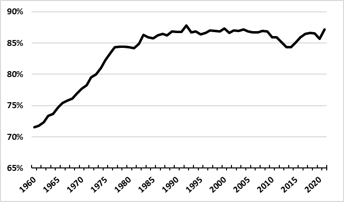
(Source: FHWA Highway Statistics, Table DL-1C)
Historically, changes in the price of gasoline have also had a pronounced effect on the demand for vehicle travel. For example, the sharp oil price spikes of the mid-1970s, early 1980s, and more recently the late 2000s, together with the accompanying economic recessions, exerted downward pressure on VMT growth, while the subsequent sharp drop in petroleum prices during the mid-1980s was partly responsible for the resumption of rapid growth in vehicle use. Other factors for which the effect on VMT growth has varied widely over time include changes in the distribution and density of the U.S. population, along with major shifts in population among regions of the country, between urban and rural locations, and within many major metropolitan areas.
To highlight these trends and accompanying changes in VMT demand, Figure 2 presents total light-duty and light-duty per capita VMT from 1966 through 2021, overlayed with recessionary periods shaded in gray. Over this period, light-duty VMT has experienced noticeable periods of strong fundamental growth, increasing more than two-fold from 1966 to 2006. When measured in per capita terms, growth in light-duty VMT was also strong, albeit with a noticeable slowdown in the trend beginning in 1990.
The sharp increase in gasoline prices beginning in 2008 combined with the subsequent deep recession and other developments to produce a prolonged period of decline and little growth in vehicle use.4 Subsequently, the steady improvement in economic activity through the mid-2010s, and decline in the price of oil, coincided with a resumption of growth in vehicle travel demand. These trends highlight the important relationship between general economic conditions and vehicle use.
Figure 2. Light-Duty Vehicle Miles Traveled (Total and Per Capita, 1966-2021)5
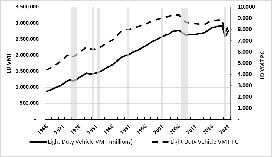
(Source: FHWA Highway Statistics, Table VM-1, Table DL-1C)
Although this discussion has focused primarily on passenger vehicle travel, developing robust approaches for modeling truck VMT is also important. Truck use represented less than 10 percent of total VMT in 2019 (Figure 3), but freight shipping is nevertheless a critical component of the nation’s transportation activity. Truck use is also an important consideration for infrastructure investment policy, since trucks are responsible for a large portion of highway wear and tear and may also contribute disproportionately to congestion and road safety conditions. Truck transportation plays a critical role in the national economy; in 2017, trucks moved 71 percent and 72 percent of all commercial freight, as measured by weight and value, respectively.6 The growth in the international trade in goods has also relied largely upon trucks to move imports and exports between U.S. coastal ports and inland production facilities and distribution centers.
Figure 3. Truck VMT as a Percent of Total VMT (1966-2021)7
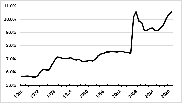
(Source: FHWA Highway Statistics, Table VM-1)
Because of the importance of freight transportation, careful consideration was given to distinguishing the factors likely to influence truck travel from those more likely to affect the use of passenger vehicles. In particular, since the demand for truck use is largely derived from shipments of raw materials to supply manufacturing facilities and distribution of finished goods, particular attention was paid to including various measures of manufacturing activity, goods production, and product delivery. These include the fraction of total economic activity accounted for by goods production, the volume of international trade, and the value of mail-order and internet sales, which substitute increased truck use for home delivery for shoppers’ travel to and from retail stores.
A major challenge in developing VMT forecasting models arises when comparing and selecting the best specification from among multiple possible alternatives (sometimes ranging into the hundreds). To meet this challenge, Volpe analysts employed a comprehensive and systematic approach to model development, evaluation, and selection.
The first step in the model development process was identifying the range of factors likely to influence vehicle use. Guided by the economic theory of travel demand, these factors were selected separately for each vehicle category: light-duty vehicles, single-unit trucks and combination trucks. Within each broad category of underlying influences on vehicle use, alternative variables measuring that influence were identified for potential inclusion in varying model formulations. For example, household income levels could alternatively be measured by total or per capita GDP, total or per capita disposable personal income, median household income, or still other measures. Table 1 summarizes the broad categories of explanatory variables and the alternative measures that were used to represent each category.
Historical data on vehicle use, demographic factors, and economic variables were drawn from a range of sources, most of which are publicly available. These include FHWA (notably, its annual Highway Statistics publication), the U.S. Energy Information Administration, R.L. Polk, the U.S. Bureau of the Census, and the U.S. Department of Labor. The historical range over which the national-level models are estimated spans 53 continuous years for light-duty vehicles and 49 years for trucks; these data series begin in 1966 and 1970 respectively, and extend through 2019.
An important category of variables potentially affecting travel activity includes those describing land use patterns; that is, measures that capture the geographic distributions of population and employment— particularly, their density within and dispersion around central cities, and their distribution between urban and suburban regions of metropolitan areas. At the nationwide level, however, no suitable measure of the influence of land use on motor vehicle travel could be identified. Candidate measures either did not display sufficient variation over time to identify their influence on vehicle use, or were inadequately or inconsistently defined at the national level throughout the historical period used to develop the models.
The economic and demographic variables selected as candidates for testing were then entered into a model specification matrix that included different possible combinations of the variables used to measure each category of influence. Using this matrix, alternative model specifications were carefully designed to test and compare how effectively each variable captured the underlying influences it was intended to measure, both individually and in conjunction with other important determinants of VMT. This allowed examination of the stability and robustness of each individual variable’s relationship to vehicle use, particularly when combined with other explanatory influences, and also enabled easy tracking of the many specifications that were tested. At the national level, approximately 300 different model specifications were examined for each vehicle class as part of this process.
| Variable Type | Light-Duty | Single-Unit Trucks | Combination Trucks |
|---|---|---|---|
| Dependent Variable | Total Annual VMT*† | Total Annual VMT | Total Annual VMT |
| Demographic Characteristics |
Total Population |
[no variables] | [no variables] |
| Economic Activity/ Income Measures |
Total GDP*† Disposable Personal Income*† Median Household Income Consumer Confidence Index Consumer Sentiment Index |
Total GDP* |
Total GDP* |
| Cost of Driving | Gasoline Price per Gallon Fuel Economy (MPG) Fuel Cost per Mile Driven |
Diesel Price per Gallon Single Unit Truck MPG Fuel Cost per Mile Driver Wages |
Diesel Price per Gallon Fuel Cost per Mile Driver Wages Combination Truck MPG |
| Vehicle Price | New Vehicle Price Index Used Vehicle Price Index Vehicle Parts and Price Index New Vehicle Price Index/Consumer Price Index New Vehicle Real Sales Price |
Producer Price Index (Transportation Equipment) New Vehicle Price Index |
Producer Price Index (Transportation Equipment) New Vehicle Price Index |
| Road Supply | Total Road-Miles*† Road-Miles per Vehicle |
Total Highway-Miles Total Highway-Miles per All Vehicles Highway-Miles in Urban Areas Percent of Population in Urban Areas |
Total Highway Miles per All Vehicles Total Highway-Miles Total Public Road-Miles |
| Employment | Total Employment Labor Force Participation Rate (%) Employed Persons per Household |
[no variables] | [no variables] |
| Transit Service | Vehicle-Miles of Bus and Rail Transit Service* Vehicle-Miles of Rail Transit Service* Number of Cities with Rail Transit Service |
[no variables] | [no variables] |
Entries marked with "*" were examined in per capita terms
Entries marked with "†" were examined in per household terms
The explanatory power and reliability of each model specification was judged based upon several statistical criteria, including:
The primary aim of this model-building procedure was to develop a model that forecasts accurately—in other words, to minimize total forecasting error. The error in the forecasts produced using a given model can be separated into two components. First, future values of the model’s explanatory (or input) variables are unknown and must themselves be forecast; “input error” refers to the component of error in the model’s forecast that can be attributed to imperfect predictions of its input variables. Minimizing such input error will tend to favor the development of parsimonious models: the smaller the number of input variables a model includes, the lower the combined uncertainty of the predictions of these variables.
“Specification error,” on the other hand, is the component of error inherent in the design and calibration of a particular model. This error reflects how well the variables it includes (and the relationships expressed by their estimated coefficients) capture the “true” determinants of the dependent variable. If a model is poorly designed— for example, if it excludes important variables, includes variables that do not belong, or its functional form causes it to understate or exaggerate the contributions of certain explanatory variables— the forecasts it produces will exhibit high specification error, even when they are generated with perfect foresight about the model’s input variables.
Minimizing specification error would generally lead the model developer to include more, rather than fewer, explanatory variables, so as not to omit any important influences from the model. Thus, attempts to reduce each source type of potential error will frequently entail conflicting recommendations for the model-building procedure.
The emphasis during the testing process was placed on models exhibiting the lowest level of specification error. In isolating the magnitude of specification error from that of input error, the mean absolute percentage error (MAPE) statistic is a particularly useful tool. The relative extent of the two error components for a given model can be examined by comparing the MAPEs calculated from out-of- sample and in-sample forecasting tests. Specifically, the accuracy of a model’s in-sample “forecasts,” which are constructed using the actual historical values of its explanatory variables, provides a measure that isolates of its specification error.
Specification error was also examined by using the models to generate out-of-sample forecasts, which are constructed using the known values of the explanatory variables to forecast VMT for part of the historical period over which the full model was calibrated. The model’s accuracy can then be examined by comparing its forecasts of vehicle use against their actual values for this part of the historical analysis period. The final model selection process aimed to ensure high forecasting accuracy, while also ensuring the structural integrity of the model by including all theoretically influential and significant factors.
During the model development process, particular attention was paid to issues that commonly arise due to the time series nature of historical demographic and economic data. One particular concern is the presence of autocorrelation in the residuals of an econometric equation, which occurs when the unexplained residual or error terms in successive time periods are correlated. Another concern is the potential existence of strong underlying time trends or unit roots in the individual variables used to estimate model parameters, and the potential for accompanying cointegration between the model’s dependent variable and its explanatory variables. In the presence of unit roots and cointegration, relying on standard statistical estimation and diagnostic methods may lead to developing models that appear reliable, but embody spurious associations rather than stable behavioral relationships.
If autocorrelation is present, regression coefficients will be inefficiently estimated (although their estimates remain unbiased), normal significance tests are not valid, and the performance of the forecast from the equation is not as robust as it could be. Autocorrelation can occur if the model’s specification does not accurately reproduce year-to-year fluctuations in the value of its dependent variable over time, or conversely, if the model predicts more year-to-year variation in its dependent variable than has actually occurred over history.
Remedies for autocorrelation, which were examined and used during the model building process, include introducing a lagged dependent variable into the equation, adding an autoregressive term, or estimating the equation in differences to make the time series data stationary. Tests for autocorrelation were conducted post-estimation using the Cumby-Huizinga general test and are reported with the regression output.8
The absence or presence of a unit root is one way to characterize the underlying temporal structure of a data series. The absence of a unit root essentially means that the data series lacks a trend, and instead varies around a stable mean; such a variable is referred to as stationary. Its average may be positive, negative, or zero, as long as it remains approximately constant. Conversely, the presence of a unit root implies that the variable is non-stationary, with its mean or expected value rising or declining consistently over time, thereby producing a historical trend in its value. The existence of unit roots is often discussed in terms of whether the series is “integrated”; a series is describes as integrated of order one when the first difference of the variable is itself stationary, or the difference between its values in successive time periods is roughly constant.
Many of the economic variables included in the models have unit roots (or are integrated of order one); in practical terms, these series typically show steady upward trends over time.9 A similar pattern can be seen in the dependent variable (vehicle use, as measured by VMT) as well. In the presence of unit roots, the standard errors estimated via the models may be inaccurate, leading to improper inference about the statistical significance of the model’s estimated coefficients. More importantly, estimated relationships that fit the data well and appear to reflect causal association may in fact be spurious if their variables have unit roots and this is not recognized when developing candidate model specifications.
Cointegration is a concern related to the unit root issue; while the presence of a unit root is a characteristic of an individual variable, cointegration is a property of multiple variables. In essence, two variables that each have unit roots but share a common underlying trend are said to be cointegrated, in the sense that they tend to increase (or decline) over time in a consistent pattern.10 Thus, growth in one of two cointegrated variables can appear to cause the other to grow, when in fact they simply happen to share similar underlying trends and their apparent relationship is spurious.11
Nevertheless, cointegration can provide useful information regarding the long-run equilibrium relationship between two variables. The fact that they share underlying trends means that the value of one variable may be useful in producing a more reliable prediction of the value of the other, although the resulting prediction is of course still prone to random variation. Estimating and utilizing cointegrating relationships offers an alternative to differencing time series as a means of resolving the problems that unit roots can introduce. That is, if cointegrating relationships are detected among the variables included in a proposed model specification, they can sometimes be exploited to capture the relationship between the model’s dependent and explanatory variables more reliably, and thus to improve the model’s forecasting performance.12
During the model development process, each variable was first tested for the presence of a unit root. Extensive testing was then conducted to detect the existence of cointegration between pairs of variables displaying unit roots, focusing particularly on cointegration between the VMT measures to be used as dependent variables in the models and the candidate explanatory variables listed previously in Table 1.13 These tests indicated the presence of unit roots in some variables, as well as some degree of cointegration among the variables included in many of the proposed model specifications.
Accordingly, alternative econometric estimation procedures were tested for their effectiveness in using cointegrating relationships to improve these specifications and identify models that produced more reliable forecasts. These alternative approaches included estimating single-equation error correction models (ECM), autoregressive distributed lag (ARDL) models, multi-equation vector autoregression (VAR), and vector error correction models (VECM). Of these various time series modeling approaches, the ARDL models proved superior in terms of robustly modeling the cointegrating relationship between VMT and the set of macroeconomic variables used to explain its historical growth.
The ARDL approach has the advantage of capturing both the long-term relationships and short-term dynamics of the relationships between the dependent and independent variables. Allowing for the model to capture the short-term dynamics has the added benefit of making the model more robust to autocorrelation, since the short-term effects of the model’s explanatory variables on its dependent variable are directly incorporated in the model’s specification and are no longer left to be subsumed in its error term. In addition, the bounds test can be utilized after estimating the error correction form of the model to confirm the existence of cointegrating relationships as an alternative to other, more complex pre-modeling cointegration tests.14
Forecasts of the models’ explanatory variables come from three sources: S&P Global Market Intelligence (formerly IHS Markit), the U.S. Energy Information Administration (EIA), and the Volpe Center. S&P Global provides many of the variables used for forecasting national VMT, while the Volpe Center developed independent forecasts of road supply and truck fuel efficiency. Volpe’s initial forecasts employed growth rates of light-duty fuel efficiency that were developed for NHTSA as part of its analysis of future Corporate Average Fuel Economy (CAFE) standards; subsequently, information from EIA has also been incorporated to project future changes in fleet fuel efficiency. Both S&P Global and EIA provide scenario-based forecasts (i.e., a baseline plus high and low growth outlooks). The Volpe- produced forecasts are not constructed around the same scenarios but can be modified to produce alternative future outlooks.
S&P Global provides forecasts for three potential macroeconomic outlooks, referred to as the baseline, optimistic, and pessimistic scenarios. The optimistic and pessimistic scenarios are to be considered relative to the baseline. The optimistic scenario reflects relatively high U.S. economic growth and low world oil prices, while the pessimistic scenario combines relatively low domestic economic growth with high world oil prices. Table 2 shows the forecast growth rates of several important aggregate economic indicators in the baseline scenario compared to historical growth rates.15
| Demographic and Economic Indicators | Historical Growth Rate16 | Forecast Growth Rate: 2019-2049 |
|---|---|---|
| U.S. Population17 | 1.0% |
0.4% |
| Total GDP (Real 2012$) | 2.6% |
1.8% |
| Disposable Personal Income per Capita (Real 2012$) | 1.8% |
1.8% |
| Imports and Exports of Goods (Real 2012$) | 5.4% |
2.3% |
| Consumption of Other Non-Durable Goods18 (Real 2012$) | 3.2% |
2.6% |
| Gasoline Price per Gallon (Real 2012$) | 0.7% |
0.2% |
The FHWA travel forecasting system includes separate models to forecast nationwide total vehicle-miles traveled by three separate vehicle classes: light-duty vehicles (automobiles plus light trucks used primarily as passenger vehicles), single-unit trucks, and combination trucks. All models use an ARDL specification.19
Each model includes one or more measures of the level and composition of the specific components of economic activity that are likely to affect demand for personal travel or freight shipping. For example, truck usage is influenced by the fraction of GDP accounted for by specific economic sectors such as manufacturing, construction, and international trade. Similarly, light-duty vehicle use is partly a product of real personal disposable income, since this variable influences household members’ opportunities to participate in activities that require travel away from home. Household characteristics such as average size, number of children, age distribution of members, metropolitan location, and distribution by geographic region were also expected to affect the volume of light-duty vehicle travel, but their effects generally proved difficult to identify at a national aggregate level.
Each model also includes a measure of fuel cost per mile driven, which is equal to fuel price per gallon divided by average fuel economy in miles per gallon for the relevant vehicle class. This variable is intended to capture the fuel-related cost of driving, which is typically the largest component of the total variable cost of operating each type of vehicle. Although there are several alternative measures of fuel- related costs, fuel price divided by fuel efficiency is preferred because it accurately reflects the independent influences of both fuel prices and fuel efficiency on vehicle operating costs.20 The effects of vehicle purchase prices and ownership costs on aggregate vehicle use were also tested in the VMT forecasting models for each vehicle class, but the influence of these variables on vehicle use was difficult to detect.
Measures of aggregate highway mileage or average highway miles per registered vehicle were also tested in the national-level VMT forecasting models for single-unit and combination trucks. These variables were intended to capture the effect of road capacity and the intensity with which it is utilized on travel speeds, which in turn are expected to influence demand for personal travel and freight shipping. Again, however, their influence on VMT could not be detected reliably. Measures of the supply and prices of competing travel modes - public transit service levels and fares, as well as rail shipping rates - were also tested for their influence on aggregate light-duty vehicle and truck use, but no such effects could be detected.
Finally, to facilitate interpretation, all model variables have been transformed into natural logarithms, which means the resulting coefficients can be interpreted as elasticities of vehicle use with respect to each model’s explanatory variables.
As Table 3 shows, the national light-duty vehicle forecasting model includes short- and long-run variables for personal disposable income per capita, average fuel cost per mile, and a short-run measure of consumer confidence in the economic outlook. Personal disposable income per capita enters the equation in linear form and with a squared term; the estimated coefficient on the linear term is positive, while that on the quadratic term is negative. This implies that personal disposable income per capita has a positive impact on VMT (that is, as household income levels rise, vehicle use per person increases), but that the magnitude of this effect declines as income continues to increase. However, recent updates to the model have shown the negative impact of the income squared term overly influencing the model, by putting substantial downward pressure on growth in the outer year of the forecast. As a result, the relationship between VMT and income was reexamined.
Figure 4. Light-Duty VMT per Capita and Real Personal Disposable Income per Capita, Index 1966=1 (1966- 2021)
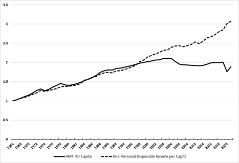
As is shown in Figure 4, both real disposable income and VMT in per capita terms grew consistently between 1966 and 2006. However, after 2006, VMT growth leveled off and even declined, while income levels continued to rise. In aggregate, this suggests that households may have reached a point where desired vehicle travel is being provided, and the relationship between VMT and income that was observed during the prior 40 years may have changed.
To examine this theory rigorously, a test for structural breaks in the relationship between VMT per capita and income per capita variables was conducted. These structural break tests consistently identified a break in the relationship in 2006.21 As a result, the light-duty vehicle VMT forecasting model now includes a structural break indicator, representing a break in the relationship between VMT and income after 2006. Prior to 2007, the indicator shows a strong relationship between income and VMT; after that period, however, there has been a “decoupling” of the relationship between income and VMT, and the income per capita variables incorporated in the light-duty VMT model include an interaction term to capture this structural change.
Table 3. Explanatory Variables Included in Light-Duty VMT Forecasting Model
| Variable | Light-Duty VMT |
| Adjustment Variable | N/A |
| LD VMT PC (-1) | -0.445 (0.055)*** |
| Long-Run Variables | N/A |
| Personal Disposable Income PC | -0.0036 (0.1015) |
| Personal Disposable Income PC x Indicator | 2.803 (0.511)*** |
| Personal Disposable Income PC Sq. x Indicator | -0.325 (0.077)*** |
| Fuel Cost per Mile | -0.094 (0.016)*** |
| Short-Run Variables (First Differenced when Δ) | N/A |
| Δ Personal Disposable Income PC | 0.015 (0.104) |
| Δ Personal Disposable Income PC (-1) | -0.291 (0.081)*** |
| Δ Personal Disposable Income PC (-2) | -0.278 (0.076)*** |
| Δ Personal Disposable Income PC (-3) | -0.148 (0.077)† |
| Consumer Confidence | 0.050 (0.016)** |
| Structural Break Indicator | -2.590 (0.566)*** |
| Constant | 3.748 (0.510)*** |
| Observations | 50 |
| Adj. R2 | 0.860 |
| Root Mean Squared Error (RMSE) | 0.008 |
| Cumby-Huizinga Test for Autocorrelation (P-Value (One Lag)) |
0.31 |
| Bounds F-Stat. | 27.289*** |
| Bounds T-Stat. | -8.059*** |
| In-Sample MAPE (1970-2019) | 0.49% |
| Out-of-Sample MAPE (2014-2019) | 0.76% |
Notes: Structural break indicator is equal to 1 prior to 2007 and 0 in 2007 onward. Suffixes on the variable names indicate the values of a variable from the previous year (-1), two years previous (-2), and three years previous (-3). Critical values for the bounds test are taken from Pesaran et al. (2001) for case 3. Model lag lengths were based on the best BIC statistic. |
|
The coefficient estimates for the disposable income variables provide further indication of the decoupling between income and VMT. When including the interaction term, the income coefficients are estimated up through 2006 and are 0 thereafter. They show the correct signs, with the linear term being positive and the squared term negative, indicating the rising opportunity cost of driving, and are highly significant in the long-run portion of the error correction model. After 2006, however, only the non- interacted income coefficient is left in the model specification, and this variable is estimated to be close to zero and is also not statistically significant. Taken together, this provides further evidence that the structural relationship between income and VMT has shifted; the model specification has been designed to explicitly capture this dynamic.22
Fuel cost per mile appears with a negative coefficient, indicating that as the cost of driving increases, households choose to travel less. As expected, higher consumer sentiment in the future of the economy is associated with an increase in the number of vehicle-miles driven per person.23
The light-duty VMT forecasting equation also includes the previous period’s value of the dependent variable as the adjustment variable in the error correction form of the ARDL. The adjustment variable has the correct negative value and is statistically significant, implying that aggregate light-duty vehicle use adjusts gradually to changes in disposable income, fuel costs, and consumer confidence. Specifically, the magnitude of its estimated coefficient suggests that the effects of changes in these factors on VMT are only partly felt in the year when they occur, and require more than 2 years to be felt completely.24 This presumably reflects the existence of structural inertia in households’ decisions affecting travel demand and vehicle use, possibly contributed by the fixed locations of their residences or workplaces and the number of vehicles they own. The bounds F- and t-statistics both confirm the presence of this long-run cointegration relationship between VMT and the macroeconomic variables.
The Cumby-Huizinga test result indicates no significant presence of serial correlation in the regression errors, ensuring that the bounds test is unbiased. In addition, the small in-sample and out-of-sample MAPEs provide a good indication of the relative forecasting accuracy of the model.
Table 4 presents the national aggregate forecasting model for combination truck (CT) VMT, which includes long-run variables of net exports of real goods and fuel cost per mile. In addition, an indicator variable is included to capture the structural break in the data generating process for CT VMT for the periods 2007 and 2008. Because the model was estimated using time series data before 1980 (1970- 1979) in the final specification, an indicator variable and its interaction with the explanatory variables are needed to capture the fact that freight trucking service was tightly regulated during that period.
As expected, the coefficient on net exports is positive, implying that growth in the trading sector of the
U.S. economy increases demand for the longer-distance shipping services typically provided using combination trucks. Fuel cost per mile appears with a negative sign, again as expected, which suggests that declining retail fuel prices or improvements in combination-truck fuel economy will also increase shipping activity using combination trucks.
Table 4: Explanatory Variables Included in Combination Truck VMT Forecasting Model
| Variable | Combination Truck VMT |
| Adjustment Variable | N/A |
| CT VMT (-1) | -0.393 (0.063)*** |
| Long-Run Variables | N/A |
| Goods Imports and Exports | 0.421 (0.016)*** |
| Fuel (Diesel) Cost per Mile | -0.096 (0.038)* |
| Short-Run Variables (First Differenced when Δ) | N/A |
| Δ CT VMT (-1) | -0.505 (0.090)*** |
| Δ Fuel (Diesel) Cost per Mile | 0.007 (0.022) |
| Δ Fuel (Diesel) Cost per Mile (-1) | -0.048 (0.019)* |
| Δ Fuel (Diesel) Cost per Mile (-2) | -0.042 (0.021)† |
| Goods Imports and Exports X Regulation Indicator | 0.587 (0.087)*** |
| Fuel (Diesel) Cost per Mile X Regulation Indicator | -0.071 (0.085) |
| Regulation Indicator | -3.788 (0.609)*** |
| Structural Break 2007/08 Indicator | 0.208 (0.018)*** |
| Constant | 3.33 (0.515)*** |
| Observations | 46 |
| Adj. R2 | 0.863 |
| RMSE | 0.019 |
| Cumby-Huizinga Test for Autocorrelation (P-Value (One Lag)) | 0.63 |
| Bounds F-Stat. | 36.469*** |
| Bounds T-Stat. | -6.218*** |
| In-Sample MAPE (1974-2019) | 1.26% |
| Out-of-Sample MAPE (2014-2019) | 2.76% |
Notes: Regulation indicator is equal to 1 prior to 1980, and 0 from 1980-2019. The bounds test critical values are taken from Pesaran et al. (2001) for case 3. Model lag lengths were based on the best BIC statistic. |
|
The adjustment variable is highly significant with the correct negative sign, implying moderate inertia in the CT carrier industry. The estimated adjustment back to the long-run equilibrium trend is roughly 2.5 years. In addition, the bounds F- and T-statistics provide clear evidence of cointegration between CT VMT and the explanatory macroeconomic variables. The Cumby-Huizinga test also provides evidence against serially correlated errors, thus validating the significant cointegration results from the bounds tests. Finally, the in- and out-of-sample MAPEs indicate good accuracy from a forecasting perspective, particularly given the shorter time series used to estimate the parameters.
National single-unit truck VMT is modeled as a function of the long-run value of fuel cost per mile, together with both short- and long-run measures of the consumption of other nondurable goods (which excludes food and energy). The model also includes two indicator variables used to capture structural breaks in the historical series for single-unit truck VMT. The first represents the structural change in the VMT series made by FHWA, which affects the values in 2007 through 2009, 25 while the second captures an apparently permanent change in the growth trend in single-unit truck use starting the following year in 2010.
Table 5 shows the model results, with both short- and long-run effects of consumption of other nondurable goods having the expected positive signs. The fuel cost per mile variable has the expected negative effect and its estimated coefficient is statistically significant. Not surprisingly, the first structural break indicator is strongly significant, since it captures the sudden increase in estimated single-unit truck VMT resulting from the change in FHWA’s data generating process. The additional structural break indicator reflects the change in the trend in single-unit truck VMT following FHWA’s revision of the data generating process, and also improves the model’s explanatory power significantly.
As with the combination truck model, the adjustment variable is highly significant, and its magnitude implies that long-run equilibrium is re-established within about 2.1 years of an unexpected shock. The estimated bounds F- and T-statistics provided further evidence that a long-run cointegrating relationship exists between single-unit truck VMT and the two independent variables, while the test for autocorrelation shows no evidence or concern for autocorrelation. Finally, the in- and out-of-sample MAPEs are within reasonable ranges and suggest that the model for single-unit truck VMT is well specified and has reliable forecasting capabilities.
Table 5: Explanatory Variables Included in Single-Unit Truck VMT Forecasting Model
| Variable | Single-Unit Truck VMT |
| Adjustment Variable | N/A |
| SUT VMT (-1) | -0.469 (0.065)*** |
| Long-Run Variables | N/A |
| Consumption of Other Non-Durable Goods | 0.730 (0.035)*** |
| Fuel (Diesel) Cost per Mile | -0.197 (0.050)*** |
| Short-Run Variables (First Differenced when Δ) | N/A |
| Δ SUT VMT (-1) | -0.140 (0.077)† |
| Δ SUT VMT (-2) | -0.389 (0.083)*** |
| Δ Consumption of Other Non-Durable Goods | 0.832 (0.219)*** |
| Structural Break 2007/08/09 Indicator | 0.368 (0.028)*** |
| Structural Break Indicator (2010 onward) | 0.108 (0.020)*** |
| Constant | 2.889 (0.386)*** |
| Observations | 46 |
| Adj. R2 | 0.856 |
| RMSE | 0.025 |
| Cumby-Huizinga Test for Autocorrelation (P-Value (One Lag)) | 0.98 |
| Bounds F-Stat. | 32.801*** |
| Bounds T-Stat. | -7.207*** |
| In-Sample MAPE (1974-2019) | 1.83% |
| Out-of-Sample MAPE (2014-2019) | 2.00% |
Notes: Structural break indicator is equal to 0 prior to 2010 and 1 in 2010 onward. The bounds test critical values are taken from Pesaran et al. (2001) for case 3. Model lag lengths were based on the best BIC statistic. |
|
FHWA and the Volpe Center update the parameters of these VMT forecasting models as additional data on vehicle use, demographic factors, and economic variables become available each year. In addition, the appropriateness of the specification and estimation procedure used for each model is periodically re-examined in order to identify opportunities to better explain historical variation in vehicle use and improve its forecasting performance. Whenever significant changes in model parameter values, functional forms, or statistical estimation procedures used for any of the VMT forecasting models are adopted, FHWA will issue an updated version of this report describing those changes.
FHWA employs the models described in this report to develop and issue its annual long-run forecasts of national VMT by light-duty vehicles, single-unit trucks, and combination trucks, as updated forecasts of each model’s explanatory variables are issued by S&P Global and developed by the Volpe Center. These forecasts, together with a brief description of the underlying economic outlook on which they rely, are available at: https://www.fhwa.dot.gov/policyinformation/tables/vmt/vmt_forecast_sum.cfm.
Cumby, Robert E., and John Huizinga. “Testing the Autocorrelation Structure of Disturbances in Ordinary Least Squares and Instrumental Variables Regressions.” Econometrica 60, no. 1 (January 1992): 185—95.
Ditzen, Jan, Yiannis Karavias, and Joakim Westerlund. “Testing and Estimating Structural Breaks in Time Series and Panel Data in Stata.” Discussion Papers, Discussion Papers, October 2021. https://ideas.repec.org//p/bir/birmec/21-14.html.
Engle, Robert F., and Clive W.J. Granger. “Co-Integration and Error Correction: Representation, Estimation and Testing.” Econometrica 55, no. 2 (1987): 251-76.
Federal Highway Administration. “Office of Highway Policy Information: Highway Statistics Series, Table DL-1C,” https://www.fhwa.dot.gov/policyinformation/statistics.cfm.
Federal Highway Administration. “Office of Highway Policy Information: Highway Statistics Series, Table VM1,” https://www.fhwa.dot.gov/policyinformation/statistics.cfm.
Federal Highway Administration. “Office of Highway Policy Information: Traffic Monitoring Guide, Appendix C. Vehicle Types,” https://www.fhwa.dot.gov/policyinformation/tmguide/tmg_2013/vehicle-types.cfm.
Hensher, D. A., F. W. Milthorpe, and N. C. Smith. “The Demand for Vehicle Use in the Urban Household Sector. Theory and Empirical Evidence.” Journal of Transport Economics and Policy 24, no. 2 (1990).
Pesaran, M. Hashem, and Yongcheol Shin. “An Autoregressive Distributed-Lag Modelling Approach to Cointegration Analysis.” In Econometrics and Economic Theory in the 20th Century: The Ragnar Frisch Centennial Symposium, edited by Steinar Strøm. Cambridge: Cambridge University Press, 1999.
Pickrell, Don H. “Description of VMT Forecasting Procedure for ‘Car Talk’ Baseline Forecasts.” U.S. Department of Transportation Volpe Center, 1995.
Polzin, Steven Edward and University of South Florida. Center for Urban Transportation Research. “The Case for Moderate Growth in Vehicle Miles of Travel: A Critical Juncture in U.S. Travel Behavior Trends,” 2006.
U.S. Department of Transportation, Bureau of Transportation Statistics, and U.S. Department of Commerce, U.S. Census Bureau. “2017 Commodity Flow Survey Final Tables,” 2020. https://www2.census.gov/programs-surveys/cfs/data/2017/.
1 Federal Highway Administration. “Office of Highway Policy Information: Traffic Monitoring Guide, Appendix C. Vehicle Types,” https://www.fhwa.dot.gov/policyinformation/tmguide/tmg_2013/vehicle-types.cfm.
2 For example, see D. A. Hensher, F. W. Milthorpe, and N. C. Smith, “The Demand for Vehicle Use in the Urban Household Sector. Theory and Empirical Evidence,” Journal of Transport Economics and Policy 24, no. 2 (1990).; Don H. Pickrell, “Description of VMT Forecasting Procedure for ‘Car Talk’ Baseline Forecasts” (U.S. Department of Transportation Volpe Center, 1995).; and Steven Edward Polzin and University of South Florida. Center for Urban Transportation Research, “The Case for Moderate Growth in Vehicle Miles of Travel: A Critical Juncture in U.S. Travel Behavior Trends,” 2006.
3 More specifically, if the annual VMT per licensed driver had remained at its 1950 level, growth in the number of licensed drivers would have resulted in half of the growth in total annual VMT that actually occurred between 1950 and 1960.
4 According to the National Bureau of Economic Research the recession started in December 2007 and ended in June 2009. Total non-farm employment in the U.S. did not return to its prerecession peak until May 2014.
5 Shaded areas note U.S. recessions.
6 U.S. Department of Transportation, Bureau of Transportation Statistics and U.S. Department of Commerce, U.S. Census Bureau, “2017 Commodity Flow Survey Final Tables,” 2020, https://www2.census.gov/programs-surveys/cfs/data/2017/.
7 The sharp spike in truck VMT in 2007 is due to a change in FHWA reporting of VMT. This change was accounted for during the forecast model development process.
8 Robert E. Cumby and John Huizinga, “Testing the Autocorrelation Structure of Disturbances in Ordinary Least Squares and Instrumental Variables Regressions,” Econometrica 60, no. 1 (January 1992): 185-95.
9 Similarly, a variable is integrated of higher orders when the variable must be differenced more than once to produce a stationary series. Nonetheless, series that are integrated of more than order one are uncommon in econometric analysis.
10 Technically, two non-stationary variables are cointegrated if there exists a linear combination of the variables that is stationary. For example, if two series x and y are integrated of order one, but a third variable z can be created as some linear combination of x and y (say, the difference between x and y) and has no unit root itself, then x and y are cointegrated.
11 Robert F. Engle and Clive W.J. Granger, “Co-Integration and Error Correction: Representation, Estimation and Testing,” Econometrica 55, no. 2 (1987): 251-76.
12 The usual procedure for doing this is to use the residual terms from estimated cointegrating relationships, which provide a measure of the extent to which the values of two cointegrated variables during a specific time period diverge from their common underlying trends, as additional explanatory variables in a model relating changes in the same two variables to each other. Because cointegrating relationships in theory capture useful information about long-term equilibrium relationships between variables, exploiting these relationships in constructing models is often preferable to simply differencing the individual series and using their differenced values to estimate the relationship between their period-to-period changes.
13 The augmented Dickey-Fuller test was used to check for the presence of unit roots in individual variables. The Engle-Granger test was relied on to detect cointegration between individual pairs of variables, while the more complex Johansen test was used to analyze the presence of multiple cointegrating relationships.
14 M. Hashem Pesaran and Yongcheol Shin, “An Autoregressive Distributed-Lag Modelling Approach to Cointegration Analysis,” in Econometrics and Economic Theory in the 20th Century: The Ragnar Frisch Centennial Symposium, ed. Steinar Strøm (Cambridge: Cambridge University Press, 1999).
15 These data are from the S&P Global March 2023 U.S. Macro long-term forecast.
16 Historical data: 1989 through 2019
17 The S&P Global population forecast is based on the U.S. Census Bureau’s long-term population projections.
18 The indicator for other non-durable goods refers to commodities such as pharmaceutical and other medical products, recreational items, household supplies, and magazines and newspapers.
19 Forecasting bus VMT is difficult due to the fact that buses serve several distinct markets, each with different influences on demand: urban public transit, intercity coach travel, charter and commuter service, and school travel. As a result, a bus VMT forecasting model is not part of the FHWA VMT forecast models.
20 This specification implies that the effects of variation in fuel prices and average fuel economy on the demand for vehicle use are equal in magnitude but opposite in direction. While some research suggests that fuel prices and fuel efficiency may have different effects on vehicle use; when these variables were entered separately the estimated magnitudes of their effects did not differ significantly from each other for any of the vehicle classes.
21 Jan Ditzen, Yiannis Karavias, and Joakim Westerlund, “Testing and Estimating Structural Breaks in Time Series and Panel Data in Stata,” Discussion Papers, Discussion Papers, October 2021, https://ideas.repec.org//p/bir/birmec/21-14.html.
22 The negative signs on the lagged short-term coefficients for personal disposable income reflect the short-run adjustments to the mean trend value of light-duty VMT resulting from exogenous changes to income during previous periods.
23 This variable enters the model exogenously in levels and is excluded from the long-run portion.
24 The adjustment coefficient of -0.445 equates to an approximate 2.25-year adjustment back to a long-run equilibrium trend.
25 This indicator variable is expanded an additional year (2009) to capture any residual autocorrelation from the structural break in the VMT series.

