U.S. Department of Transportation
Federal Highway Administration
1200 New Jersey Avenue, SE
Washington, DC 20590
202-366-4000
Federal Highway Administration Research and Technology
Coordinating, Developing, and Delivering Highway Transportation Innovations
| REPORT |
| This report is an archived publication and may contain dated technical, contact, and link information |
|
| Publication Number: FHWA-HRT-12-072 Date: May 2013 |
Publication Number: FHWA-HRT-12-072 Date: May 2013 |
This chapter focuses on evaluating the performance of the sensor for fatigue testing. The main objective is to develop a robust data interpretation algorithm that is able to use the diminished data provided by the sensor to achieve reasonable predictive capabilities comparable to what is obtained using conventional measuring techniques (conventional strain gauges). The time compressed cumulative data provided by the sensor result in a loss of information. A set of laboratory tests were designed to quantify and characterize the effect of these losses. The objective is to recreate the damage index variation curves using only the cumulative information tracked by the sensor.
Measured peak strain distributions in a pavement are approximated by Gaussian distributions for all of the considered cases. The variation of the strain amplitude over time is due to the increase of the compliance (i.e., induction of fatigue damage in the specimen). Figure 168 shows the strain amplitude variation of a concrete beam over time under cyclic loading at a constant amplitude. The strain amplitude is shown to increase, which explains the loss in the elastic modulus of the beam. This increase in amplitude causes the increase of the output voltage amplitude that is recorded by the sensor.
The considered hypothesis is that a shift in the measured strain distributions toward higher strains over time is indicative of damage accumulation. Thus, monitoring the mean and the standard deviation of the distribution over time and tracking the mean variations allow researchers to determine the levels of strains that are induced in the specimen between reading periods. By determining these response levels, the compliance can be evaluated. A simplified model, described in this section, shows how these measurements are obtained and related to damage.
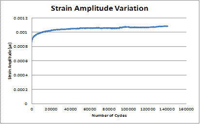
Figure 168 Graph. Strain amplitude variation of a concrete beam under cyclic load with constant amplitude.
The strain cumulative density function (CDF) is characterized by figure 169 as follows:
![]()
Figure 169 . Equation. Strain cumulative density.
Where:
μ= Mean of the strain distribution.
σ= Standard deviation reflecting the width of the normal distribution.
β= Total cumulative time of applied strain.
The sensor output data are defined by these three parameters, which are obtained by fitting the sensor's output distributions collected from all the memory cells.
Figure 170 shows the measured strain CDF from the sensor at different life stages of the beam. The amplitude is expressed in voltage, which is directly related to the event's cumulative durations.
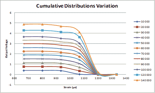
Figure 170. Graph. Cumulative distribution of strain expressed in voltage.
The shift of the mean due to the strain amplitude variation cannot be directly obtained from the cumulative distributions. Figure 171 shows the normalized density distribution reconstructed from the measured CDF at different life stages. The mean of the distributions is equal to the average induced strains amplitude, thus proving the consistency of the assumptions.
To determine the final design of the sensor, the number of gates per sensor was evaluated using a sensitivity analysis. Figure 172 shows the variation of the relative error per gate versus the sensor strain level for different specimens at different life stages. Starting from eight gates per sensor, the relative error is less than 1 percent.
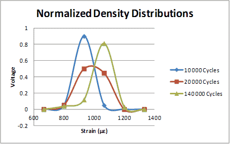
Figure 171. Graph. Normalized density distribution expressed as normalized voltage.
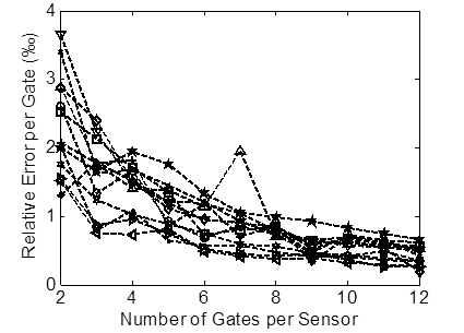
Figure 172. Graph. Relative error of fitting per gate for specimens at different life stages versus number of gates per sensor.
Due to the missing load data and the fact that the output response is collected periodically (e.g., once every year), the damage index cannot be evaluated as a deterministic value. In this project, the damage index is considered to be the ratio of the elastic moduli of the beam at any time, t, with respect to a predefined initial condition (baseline). The sensor output, as defined in figure 169, is a cumulative distribution of multiple normally distributed strain histograms defined by the equation in figure 173.

Figure 173. Equation. Cumulative distribution.
The standard deviation, the cumulative loading time, and the mean of the cumulative strain are evaluated from the parameters of the strain loading distributions shown in figure 174 through figure 176.
![]()
Figure 174. Equation. Cumulative loading time.
![]()
Figure 175 . Equation. Mean of the cumulative strain.
![]()
Figure 176. Equation. Standard deviation.
Using figure 175 and figure 176, the mean and the standard deviation of the applied strain amplitude at a time t can be evaluated using two consecutive readings, as expressed by the following equations in figure 177 and figure 178.
![]()
Figure 177. Equation. Mean of the applied strain amplitude at time t.

Figure 178. Equation. Standard deviation of the applied strain amplitude at time t.
Once the mean and the standard deviation of the strain distributions are evaluated, Taylor series with exact derivation are used to derive the mean and the variance of the damage coefficient, which are given by figure 179 and figure 180.
![]()
Figure 179. Equation. Mean of the damage coefficient.
![]()
Figure 180. Equation. Variance of the damage coefficient.
The reliability index, considered with respect to a damage coefficient equal to 0, is then evaluated as follows:

Figure 181. Equation. Reliability index.
The probability of failure, which is defined as the probability of the damage coefficient being less than 0, is then given by the following equation:

Figure 182. Equation. Probability of failure.
Expressing the failure of the structure in terms of probability of failure is more meaningful, given that the damage coefficient at failure is not a predefined value, and it varies from one specimen to another.
A total of 23 plain PCC three-point single-edge notched beam specimens were tested under constant and variable amplitude fatigue loading. Two beam sizes were considered: the large-sized beams had a span of 16 inches (406.4 mm), a depth of 4 inches (101.6 mm), and a width of 4 inches (101.6 mm). The small-sized beams had a span of 8 inches (203.2 mm), a depth of 2 inches (50.8 mm), and a width of 2 inches (50.8 mm). The notch to depth ratio for each specimen was 0.35. A COD gauge was used to measure the crack mouth opening and was attached to a pair of knife edges, which were mounted to the bottom face of the beam by a fast-drying epoxy resin, as recommended by Shah et al.(6) Each specimen was subjected to a 2-Hz cyclical load. Ten specimens were subjected to constant amplitude loading using a stress ratio (max load/peak load) of 0.85 and 0.95. The other specimens were subjected to variable loading in which both the R ratio (minimum/maximum load) and the stress ratio were varied at several stages throughout the test.
The concrete mix used in this research consisted of ASTM C-150 type I cement, a natural sand, and a limestone coarse aggregate (nominal maximum size of 1 inch (25.4 mm)). The water-to-cement ratio was 0.45, and the air content was 6.5 percent. The unit weight was 142 lb/ft3 (22.7 kg/m3).
The average 28-day modulus of rupture and the split tensile strength, f't, were 760 and 419 psi (5,236.4 and 2,886.91 kPa), respectively. The 28-day compressive strength was 3,626 psi (24,983.14 kPa). The specimens were cured for 1 year inside of a humidity room and then placed in ambient temperature for one more month to ensure minimal strength gain during fatigue testing.
The full strain-time history output from the COD gauge was used as an input into the damage algorithm proposed. The measured peak strain distributions monitored by the COD gauge over the entire life of the specimens under constant and variable loading can be approximated by Gaussian distributions as shown in figure 183 through figure 185. The figures show the strain distribution at different life stages of a specimen subject to variable loading. The shift of the strain amplitude over time is due to the variation of material stiffness, which happens because the material is damaged.
The same observations remain valid for strain distributions at different life stages of a specimen under constant loading. However, the standard deviation is higher under variable loading, which is expected because there is an additional strain bandwidth caused by the variation in loading amplitude (and not damage).
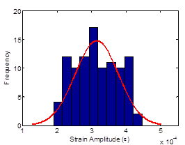
Figure 183. Graph. Strain distribution histogram at different life stages of the beam at 100 cycles.
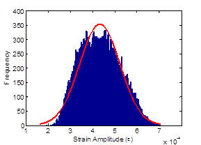
Figure 184. Graph. Strain distribution histogram at different life stages of the beam at 25,000 cycles.
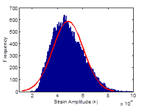
Figure 185. Graph. Strain distribution histogram at different life stages of the beam at 40,500 cycles.
Using eight gates per sensor, the cumulative strain-time distributions are fitted (see figure 186 through figure 188). Using the mean and the amplitude of the distribution, the actual induced strains distribution can be evaluated using figure 177 and figure 178. The initial mean strain (µo) is evaluated at the initial stage of specimen life (less than 100 cycles). Approximation of the extent of damage can thus be obtained.
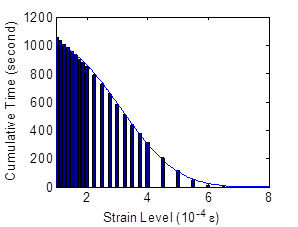
Figure 186. Graph. Fitting the sensor's output at different life stages of the specimen at 100 cycles.
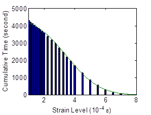
Figure 187. Graph. Fitting the sensor's output at different life stages of the specimen at 25,000 cycles.
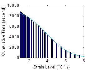
Figure 188. Graph. Fitting the sensor's output at different life stages of the specimen at 40,500 cycles.
Figure 189 shows the variation of the damage coefficient distribution versus the number of applied load cycles. The accumulation of damage is shown as a decrease of the damage coefficient mean value and a flattering of the distribution, explained by the increase of the uncertainty. As shown in figure 189, the mean damage index is decreasing over time, which is inversely proportional to the strain amplitude variation. However, the variance of the distribution is almost constant over the lifetime, with a fast change at the failure stage of the beam explained by important variability of the induced stain during failure. Once the standard deviation and the mean are evaluated, the reliability index and the probability of failure can be calculated using figure 181 and figure 182.
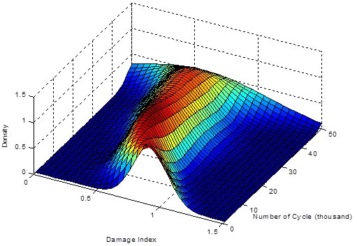
Figure 189. Graph. Probability distribution of the damage coefficient versus the number of cycles of loading.
Figure 190 through figure 193 show the variation of the reliability index of the damage coefficient as well as the probability of failure versus the number of cycles.
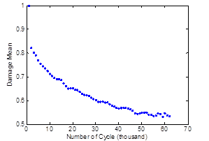
Figure 190. Graph. Variance damage coefficient distribution.
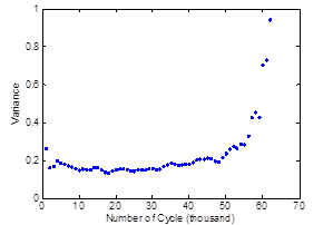
Figure 191. Graph. Variation of the mean.
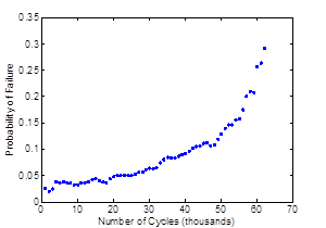
Figure 192. Graph. Probability of failure of one of the samples versus the number of load cycles.
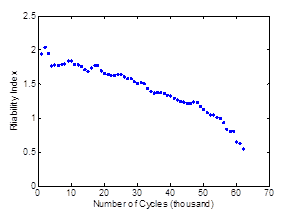
Figure 193. Graph. Reliability index of one of the samples versus the number of load cycles.
Researchers estimated remaining life of the host structure using only the compressed data from the sensor and the models discussed in section 6.2. The evaluation of the deterministic values of the damage coefficient based only on the mean value has proven to be an unreliable indicator of remaining life. This is due to the high variability of the coefficient around failure.
Table 5 shows the reliability index, the damage coefficient, and the probability of failure just before failure. Due to the high variability of the damage index at failure, the probability of failure just before failure and the reliability index are not consistent. For a better remaining life estimation, the damage index variability at failure needs to be accounted for.
Table 5. Reliability index, probability of failure, and damage coefficient at failure for different specimens.
Sample |
Reliability Index at Failure |
Probability of Failure Just Before Failure |
Damage Coefficient at Failure |
1 |
0.54 |
0.29 |
0.3 |
2 |
0.77 |
0.25 |
0.44 |
3 |
0.72 |
0.31 |
0.56 |
4 |
0.51 |
0.31 |
0.46 |
6.3.1 Mechanistic-Empirical Approach
Figure 194 and figure 195 show the linear damage accumulation rule that is used in mechanistic-empirical (M-E) models. The coefficients,βi, are calibrated for every specimen using the sensor damage reading at the damage inflection point. Subramaniam et al. observed that under constant amplitude loading, the inflection point between the deceleration and the acceleration cracking region occurs at approximately 40 to 50 percent of the total life of the specimen.(7) Thus, the coefficients pertaining to the first half of the specimen's life should be similar to the second half. Once the coefficients are known, a remaining life prediction can be made.
![]()
Figure 194. Equation. Linear damage accumulation rule.
![]()
Figure 195 . Equation. Remaining life.
Table 6 shows the predicted remaining life using the described method based on the sensor output (models described in section 6.2) and based on the calibrated coefficient of the linear damage accumulation rule for different tested specimens. The loading of the specimens was stopped, and the remaining life was estimated using the different methods and based on the evaluated damage at that stage. The tests were then continued until failure in order to record the actual remaining life. As observed in the results, for the considered cases, the predictions evaluated using the localized sensor data are closer to reality than linear damage accumulation predictions based on averaged values.
Table 6. Predicted remaining life cycles using M-E calibrated coefficients and using the updated sensor output.
Exact Remaining Life (Loading Cycles) |
Predicted Remaining Life Using Linear Damage Accumulation (Loading Cycles) |
Predicted Remaining Life Using the Sensor (Loading Cycles) |
391 |
709 |
325 |
20,527 |
716 |
5,873 |
420 |
835 |
425 |
9,350 |
902 |
7,125 |
7,022 |
922 |
11,048 |
10,980 |
990 |
23,011 |
6.3.2 Probabilistic Approach
Reliability engineering and survival analysis mostly deal with a positive random variable called "lifetime." The lifetime is manifested by a failure or other end event. In this case, failure is defined by the total break of the beam, and the lifetime variable is the time, T, at which the failure occurs with a cumulative distribution function F(T), defined by the probability of the damage index at time T being higher than the damage index at failure, as seen in figure 196.
![]()
Figure 196. Equation. Cumulative distribution function.
Figure 197 shows the density function of the damage coefficient at failure. A total of 63 specimens have been tested, and the index has been measured using COD. The fitted distribution is a logit-normal distribution.
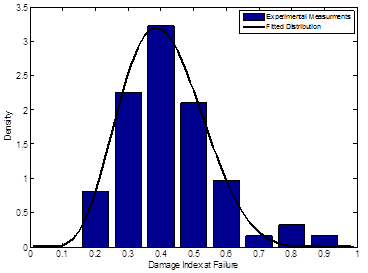
Figure 197. Graph. Probability density function of the damage index at failure.
Researchers evaluated the survival probability function of the specimens based on the evaluated damage index obtained using the sensor and also evaluated the probability density function of the index at failure.
The remaining life CDF is defined using the law of conditional probability, the condition being that the beam did not fail at time t = x.
![]()
Figure 198. Equation. Remaining life CDF.
The corresponding survival probability function of the beam is given by the following equation:
![]()
Figure 199. Equation. Survival probability function of the beam.
Remaining life is then estimated to be the expectation of the survival probability function:
![]()
Figure 200. Equation. Expectation of the survival probability function.
However, the life probability function is not defined.
Remaining life should be expressed as a function of the damage index probability function (the only information that the sensor can provide). Using a change of variable, figure 199 can be expressed as a function of the damage index.

Figure 201. Equation. Function of the damage index.
Where dD/dt is the variation of the damage index with respect to time evaluated by fitting a shape function to the discrete values evaluated using the sensor. The assumed shape functions are linear, exponential, and arcsine.
Figure 202 shows the normalized predicted remaining life (see figure 201) derived using the developed methodology based solely on the sensor's output. The associated probability (from figure 198) is shown in figure 203. As the number of applied cycles increases, more readings are incorporated into the adaptive models, which are used as fitting points. This implies that as the specimen gets closer to failure, the prediction accuracy improves, which is shown by the higher probability (reliability) of the estimated remaining life.
As discussed, the probability of the remaining life is a good indicator of predictions reliability. As shown in table 7, for a probability higher than 0.6, the relative error of the predicted remaining life is less than 50 percent.
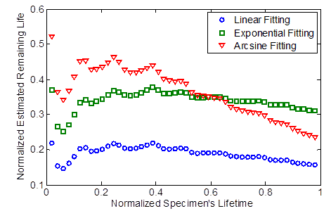
Figure 202. Graph. Normalized estimated remaining life versus the normalized specimen's lifetime using three fitting shape functions.
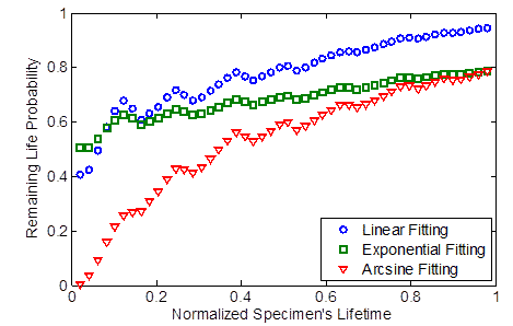
Figure 203. Graph. Remaining life probability versus normalized specimen's lifetime using three fitting shape functions.
Table 7. Estimated remaining life using the different fitting shape function.
Exact Remaining Life |
Exponential Shape Function |
Linear Shape Function |
Arcsine Shape Function |
||||||
Remaining Life |
Prob. |
Error (Percent) |
Remaining Life |
Prob. |
Error (Percent) |
Remaining Life |
Prob. |
Error (Percent) |
|
0.9 |
0.1809 |
0.6406 |
71.91 |
0.3003 |
0.6071 |
59.97 |
0.4064 |
0.2133 |
49.36 |
0.8 |
0.2014 |
0.6565 |
59.86 |
0.3435 |
0.6149 |
45.65 |
0.4347 |
0.3459 |
36.53 |
0.7 |
0.2026 |
0.6913 |
49.74 |
0.3539 |
0.6309 |
34.61 |
0.4207 |
0.4346 |
27.93 |
0.6 |
0.2116 |
0.7688 |
38.84 |
0.3703 |
0.6746 |
22.97 |
0.4221 |
0.5455 |
17.79 |
0.5 |
0.2031 |
0.807 |
29.69 |
0.3629 |
0.6959 |
13.71 |
0.3881 |
0.5988 |
11.19 |
0.4 |
0.1919 |
0.8444 |
20.81 |
0.3496 |
0.717 |
5.04 |
0.3481 |
0.6436 |
5.19 |
0.3 |
0.1796 |
0.8751 |
12.04 |
0.3368 |
0.735 |
3.68 |
0.3115 |
0.6784 |
1.15 |
0.2 |
0.1719 |
0.9068 |
2.81 |
0.3287 |
0.7575 |
12.87 |
0.2836 |
0.7218 |
8.36 |
0.1 |
0.1617 |
0.9315 |
6.17 |
0.3171 |
0.7748 |
21.71 |
0.2525 |
0.757 |
15.25 |
Several researchers studied the effects of traffic wander on pavement performance. (8–10) It was shown that the wheel wander is critical because it determines the distribution of load location on the pavement as well as the frequency at which a point is loaded. Measurements from a field study conducted by Timm and Priest showed that wheel wander tends to be normally distributed with a standard deviation ranging from 8 to 24 inches (203.2 to 609.6 mm). (11) Given that only a limited number of sensors can be implemented on a pavement section, it is critical to generate full field data and incorporate the effect of traffic wander in the fatigue prediction algorithms that use the data collected from the implemented sensors. In addition, the obtained full field data can be used to backcalculate the traffic wander distribution at a given location by tracking strain peaks in the generated data in a pavement cross section. These problems could be considered as missing data problems. Several techniques have been used to generate missing data from a set of measurements at a set of predetermined locations. In this report, the Kriging technique was implemented to test its applicability to the specific data collected from the developed sensors.
The novel self-powered microsensors presented in chapter 2 of this report are capable of continuously monitoring local strains of the host structure. They implement the level-crossing counting algorithm. A network of N implemented sensors will generate N random variables
(X1,...,XN)that describe the response of the system at a given state.
Examples of strain output distributions are shown in figure 204. The shown data are obtained from the model of piezo-powered sensors attached on a simply supported beam with dimensions 12 × 1 × 1 inch (304.8 × 25.4 × 25.4 mm) and subject to a random applied loading at its center, inducing a mid-span deformation of amplitude varying between 0.04 and 0.12 inches (1.02 and 3.04 mm). PZT piezoelectric generators with dimensions of 0.4 × 0.2 × 0.004 inches (10.16 × 5.08 × 0.10 mm) were used in the simulation. The generators' output were obtained at three different positions (x = 2.9, 3.7, and 4.9 inches (73.66, 93.98, and 124.46 mm)), where x is the position of the piezo-strip center measured from the left end of the beam. The cumulative strain data at each sensor node can be fit to a variation of the exponential discrete probability distribution of the form f(y)= θ1eθ2y2+θ3y, where y = (1,2,...,7) is the memory cell number also associated with a strain amplitude level, and θT = (θ1, θ2, θ3)represents the parameter of the strain distribution at a given location. The vectors θT are specific to a location and a system's condition; they are the parameters to estimate at the missing locations.
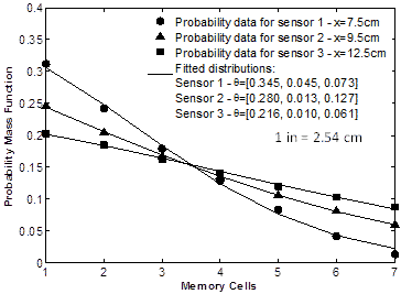
Figure 204. Graph. Example of data from distributed sensors on a simply supported beam under random loading.
In its simplest form, the basic goal of the Ordinary Kriging (OK) is to estimate the attribute value at an unobserved location by interpolating the observed values in the neighborhood locations. If (ui, i = 1…, n) at n locations in a region of interest R where the field data X has been observed, and u denotes a specified but arbitrary unobserved location in the region R, then the value to estimate X* (u) at location u is given by the following equation:

Figure 205. Equation. Estimate of X as a function of mu.
Where m(u) is the mean of X(u) and αi(u) are the Kriging weights that can be determined for the case of an OK formulation by solving the following system of equations:
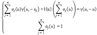
Figure 206 . Equation. System of equations to solve for the case of an OK formulation.
Where:
(ui – uj) = Distance between location i and location j.
(ui – u) = Distance between location i and the location to be estimated.
l(u) = Lagrange parameter.
y = Predefined semi-variance property that expresses the degree of spatial dependence
between points.
A simply supported beam setup was initially used to test and tune the developed techniques under simplified strain distributions; the load configuration consisted of a moving concentrated load for generating linear strains along the beam and a distributed load for quadratic strains. Simulated strain data were generated using the piezoelectric generator and the sensor models described in chapters 2 and 3. The frequency distribution of strain levels at a selected reference location (x = 3.7 inches (93.98 mm)) of the beam was estimated for different loading and known data combinations. One million cycles of random amplitude for each loading combination were simulated. Values of y in figure 206 were extracted using linear and quadratic variograms. It was determined that higher order variograms do not improve the obtained estimations for the considered strains. It was also observed that a better estimation is obtained when the missing data point is located between the known points. For example, the cumulative relative error when the known couple is located at 3.34 and 4.1 inches (84.84 and 104.14 mm) is 0.0193, while it is equal to 0.0567 for the case of a known couple at 4.1 and 5.3 inches (104.14 and 134.62 mm). The error decreases to 0.0433 for 3.34 and 5.3 inches (84.84 and 134.62 mm) even though the relative distances to the point at which an estimate is desired are the same.
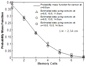
An example of estimated probabilities obtained using the Kriging technique is shown in figure 207. The probability mass function of the strain levels at the location x = 3.7 inches (93.98 mm) if a sensor was to be installed at that position is also shown. Second order polynomial variograms were used for this case. The computed errors are 0.0415, 0.0694, and 0.072, respectively, for the cases 3.34, 4.1, and 4.5 inches (84.84, 104.14, and 114.3 mm), 3.34, 5.3, and 5.7 inches (84.84, 134.62, and 144.78 mm), and 4.1, 5.3, and 5.7 inches (104.14, 134.62, and 144.78 mm).
1 inch = 2.54 cm
Figure 207 . Graph. Theoretical and estimated strain probability distributions at 3.74 inches (94.99 mm) using data from groups of three sensors at different locations.
The refined algorithms were then tested under more realistic conditions with complicated strain profiles. The objective was to prove the validity of the methods for pavement structures. The three-dimensional response of a layered system under a moving load with static and dynamic components has been modeled. The properties of the used layered system were obtained from Chabot et al.(12) The three-layered system consists of a top viscoelastic layer modeled through the Huet-Sayegh model, a road base (3.14-inch (79.76-mm) thickness), and a subbase layer (16.5-inch (419.1-mm) thickness) both assumed to be elastic and dependent on thermal and moisture characteristics.(13–16) Detailed properties are given in Chabot et al. and Nilsson et al.(12,16)
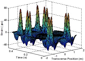
Traffic distributions were generated and applied as input loading to the pavement structure. Four different types of trucks were considered in the analysis: classes 9, 11, 5, and 16.(17) To simulate traffic wander, five different possible positions within the wheel path were selected. In total, 1,000 passing truck events were simulated. Each event corresponds to a randomly selected truck type passing at a randomly selected position within the wheel path. The loading per axle as applied in this analysis was as follows: 15,400 lb (6,991.6 kg) for steering axle, 18,000 lb (8,172 kg) for single axle, 16,000 lb (7,264 kg) for tandem axle, and 13,000 lb (5,902 kg) for tridem and higher axles. Figure 208 and figure 209 show an example of generated longitudinal strain response for the class 9 trucks at the bottom of the viscoelastic layer. The results indicate a significant interaction between the axles and relatively large tensile strains (compressive strains at the surface of the pavement). At each node location in figure 208 and figure 209, the cumulative strain data induced by randomly generated truck traffic distributions were compressed into probability mass function histograms using the piezoelectric generator and the sensor models described above. The objective of this exercise is to recreate the probability mass functions of cumulative strains induced by all the loading events at all locations within the pavement section using only a finite number of sensors implemented at determined node locations.
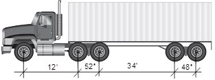
Figure 208. Illustration. Example of a class 9 truck used for strain response data generation.
1 ft = 0.305 m
Figure 209. Graph. Example of longitudinal strain profile evaluated at the bottom of the HMA layer for a moving load induced by a class 9 truck.
The frequency distribution of strain levels at a selected location 9 inches (228.6 mm) away from the center of the wheel path under the moving load is shown in figure 210. Estimated probability mass functions using two sensors placed on each side of the unknown data node are also shown. Results from known nodes at 3.93- and 7.87-inch (99.82- and 199.89-mm) spacings (1.96 and 3.93 inches (49.78 and 99.82 mm) from the location to estimate) are shown. Values of y in figure 206 were extracted using cubic variograms. It was determined that higher order variograms do not improve the obtained estimations for the considered strains.
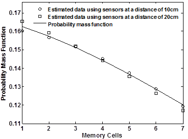
Figure 210. Graph. Theoretical and estimated strain probability distributions at a selected transverse location using data from two sensors at different spacing distances.
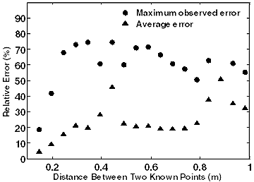
Figure 211 shows the computed relative error obtained from estimated probability distributions at all the nodes in the pavement section for different known nodes spacing distances varying from 4 to 40 inches (101.6 to 1,016 mm) (the nodes' spacing resolution is 1.96 inches(49.78 mm)). The averaged and maximum observed values are shown for each case. It can be seen that in order to achieve full reconstruction of the data in all the field points with an average error less than 10 percent, the maximum spacing between placed sensors has to be less than 7.87 inches (199.89 mm).
1 ft = 0.305 m
Figure 211. Graph. Maximum observed relative error and average relative error from generated data at all field points using known nodes at different spacing distances.
In this chapter, a sensor-specific data interpretation algorithm for predicting remaining fatigue life of a pavement structure was developed using cumulative limited compressed strain data stored in the sensor memory chip. The algorithm was verified using actual laboratory fatigue test results of a notched concrete beam under constant, variable, and random loading histories.