Pavement Performance Measures and Forecasting and The Effects of Maintenance and Rehabilitation Strategy on Treatment Effectiveness (Revised)

CHAPTER 7. LTPP DEFLECTION DATA ANALYSES

FWD DEFLECTION DATA AND RFP AND RSP

Pavement deflection data are typically collected by State transportation departments at the project level and rarely at the network level. However, most LTPP test sections were subjected to deflection testing on a periodic basis. The deflection data were collected using the most common type of equipment, the FWD. FWD tests are often preferred over laboratory testing for several reasons, including the following:^(78,83)

• FWD tests are nondestructive in nature, whereas laboratory tests require cores.
  
  
• The operational cost per FWD test is much lower than a laboratory test.
  
  
• FWD tests have short duration and can be designed to provide more coverage of the pavement network compared with laboratory tests, which are time consuming and limited to the locations where pavement cores were extracted.
  
  
• FWD data reflect the in-situ boundary conditions.

The FWD operates on two basic assumptions: the force of impact of a falling weight is considered a static load, and the roadbed soils act as an elastic body.⁽⁸³⁾ The deflection data collected from FWD testing are typically used for the following purposes:

• Backcalculating the moduli values of the pavement layers, which can be used to assess the structural capacity of the roadway and to facilitate treatment type selection and design.
  
  
• Assessing the variability of the structural capacity along and across the pavement sections.
  
  
• Analyzing LTE in rigid pavements.
  
  
• Determining the presence of voids under the pavement slabs.
  
  
• Studying the magnitude of slab curling and its impact on ride quality.

At the time of this report, research was exploring methods to increase the efficiency of deflection data collection by using a rolling wheel deflectometer (RWD). The RWD collects pavement deflection data at highway speeds and makes network-level data collection more feasible. It was reported that the results were used to flag structurally deficient pavement sections for further analyses and to estimate the structural number.^(83,84) In this study, the LTPP deflection data were analyzed to determine whether the data could be used to estimate the RSP of pavement sections and to determine the critical time for pavement preservation.

The RSP algorithm is primarily based on the measured time-dependent pavement surface condition and distress data and their corresponding threshold values. Hence, the distress (such as cracking) must be visible from the pavement surface. During the development of the RFP and RSP concepts, it was envisioned that the pavement deflection data could be used to indicate impending distress and become a part of the RSP algorithm. Such algorithms would empower State transportation departments to take corrective actions prior to the manifestation of surface defects.

To incorporate deflection into the RSP algorithm, a deflection threshold value must be developed for each pavement section. To investigate the potential for the development of deflection threshold values, the measured FWD deflection data of various LTPP test sections were analyzed as described in the next few subsections.

At the outset, it was envisioned that the rate of change and the magnitude of the measured deflections were related to the measured pavement distresses such as alligator cracking. Because alligator cracks initiate at the bottom of the asphalt layer and propagate upward toward the pavement surface, the pavement system starts to weaken as the cracks initiate and before they reach the pavement surface. Therefore, it was assumed that flexible pavement deflections would start to increase before the appearance of alligator cracking on the pavement surface (i.e., the response of a pavement structure to load would increase as the pavement deteriorated, which could be used as an early warning of impending, surface alligator cracking). Similarly, for rigid pavements, increasing the magnitude of deflection could be a sign of deterioration of the concrete slab support. Such deterioration could lead to distresses such as transverse cracking, corner breaks, and so forth. Again, increasing deflection over time may provide a flag prior to the appearance of the pavement surface distress. Further, LTE across joints or cracks in rigid pavements was typically measured using the differential deflection across joints or cracks. Increasing relative differential deflection implied lower LTE. It was also envisioned that the rate of change of LTE across joints or cracks in rigid pavements could be related to the rate of change of faulting. Joints with a good load transfer mechanism, such as dowel bars, would have almost 100‑percent LTE and little or no faulting, whereas joints without dowel bars or with damaged or sheared dowel bars, or cracks with no aggregate interlock, would have minimal LTE and increased probability of faulting. Therefore, decreasing LTE over time could be used to warn of impending surface defects.

TIME-SERIES FWD DATA MODELING—FLEXIBLE PAVEMENT

Once again, it was envisioned that an analysis of the time-series deflection data could provide indication of relationships between pavement deflection and pavement condition or distress. To investigate such potential relationships, FWD deflection data from the LTPP SMP test sections were plotted as a function of time following the procedures discussed in the following subsections. A partial record of the inventory data for the SMP test sections are listed in table 108. The deflection data were analyzed to determine trends in the measured deflection over time. Such trends, if they existed, would provide a tool for pavement managers to estimate future pavement conditions and distress before surface defects such as cracking occurred. The SMP test sections were used in this analysis because deflection data were collected on a much more frequent basis than the other LTPP test sections. However, because the FWD tests were performed at various times of the year and at different temperatures, the measured deflection was adjusted to account for the material properties and their relationships to temperature. The details of these adjustments are presented in the following subsections.

Table 108. LTPP SMP partial inventory data.

Temperature-Deflection Correlation

Some researchers have developed correlations between temperature and the measured flexible pavement deflections. At the time of this report, the most publicized temperature correlation model was that of the AI.⁽⁸⁵⁾ In this model, the measured pavement deflection basin was adjusted based on the measured pavement temperature and the untreated base thickness. Stated differently, the AI temperature adjustment factor (TAF) was used as a multiplier to adjust the entire measured deflection basin to a standard temperature of 70 ºF (21 ºC). This made the implementation of the AI method at the network level relatively easy. Other models, such as the BELLS, had also been developed and verified based on the LTPP SMP data.⁽⁸⁶⁾ These models were developed using the measured air temperatures during the FWD testing, the measured pavement surface temperatures, and the temperatures of the asphalt mat measured at various depths from the pavement surface. The use of these models facilitated the adjustment of the backcalculated layer moduli values to different temperatures. However, the data required to use the models is not readily available in the current or historic deflection records of most State transportation departments and would require additional effort to obtain.

In this study, the main purpose of the analyses of the deflection data was to identify relationships, if any, between the measured pavement deflection and the measured pavement condition data, to determine whether the deflection data could be used to estimate the optimum time for pavement preservation. To conduct the analyses, the measured pavement deflections must be adjusted to the standard temperature of 70 ºF (21 ºC). Therefore, the first step in the analyses was to validate the existing temperature adjustment models using the LTPP measured deflection data along the various SMP test sections. The analyses were based on the measured pavement deflections and surface temperature, the data most commonly collected by State transportation departments. Please note that at the time of this report, most State transportation departments did not collect network level deflection data, however, that may change in the near future as more efficient deflection measuring techniques are developed. Nevertheless, the temperature adjustment analyses were based on network level assessments, in conjunction with the RFP/RSP concepts developed in this study. After the analyses of the temperature adjustment models, backcalculation of layer moduli were performed at the project level.

The AI method for temperature adjustment of the measured deflection data could be relatively easily applied to network-level deflection data. As stated earlier, the AI method (see figure 67) provided TAFs to be multiplied by the measured deflection basin based on the mean pavement temperature and the thickness of the untreated base layer.

©Asphalt Institute
1 inch = 25.4 mm.
ºF = 1.8 × ºC + 32.

Figure 67. Graph. AI TAF.⁽⁸⁵⁾

To assess the accuracy and applicability of the AI TAFs, the measured LTPP deflection data along several SMP test sections were analyzed to determine the TAFs at each site using the following steps:

• Step 1: For each of the SMP test sections listed in table 108, the FWD measured deflection data, treatment history, and the inventory data were downloaded from the LTPP Standard Data Release 28.0. The corresponding measured pavement surface temperature at the time of each test was paired with the deflection data for analyses.
  
  
• Step 2: The measured deflection data were first analyzed and their variability along the test sections and linearity with the load magnitude were scrutinized to produce the following findings:
  
  
  • A linear relationship existed between the drop loads and the measured deflections.
    
    
  • The measured deflections along a given test section were variable.
    
    
  • The percent variability of the deflection data was more or less equal across the seven FWD sensors and in each climatic region.
    
    
• Step 3: The data were sorted based on the applied load and the various test locations along the test section. Drop height 2, which simulated the application of a 9,000-lbf (40‑kN) half single axle load, was selected for analyses. The tests performed at the mid-lane (F1) and outer wheelpath (F3) locations were selected for individual analyses. All data from other test loads and locations were not included in the analyses.
  
  
• Step 4: On any particular test day, a series of 4 tests were conducted at drop height 2 and at about 10locations along the test section. Note that tests conducted when the temperature was below freezing were not included in the analyses because the response to load is significantly different for frozen soils. On some days, the test sections were subjected to more than one series of tests. The various deflection tests conducted on a test section within each specific testing day were averaged along with the measured pavement surface temperatures to simulate the data that would be collected by a State transportation department (only one test per section). Note that the data averaging generally produced a less than 1-percent error and was dependent on the variability of the measured data.
  
  
• Step 5: The average peak deflection measured at sensors 1 through 7, located at 0, 8, 12, 18, 24, 36, and 60 inches (0, 203, 305, 457, 610, 914, and 1,524 mm), respectively, from the load, were plotted against the measured pavement surface temperatures. The deflection measured beneath the load (d₁) was composed of the response from all pavement layers; at 8 inches (203 mm) from the load (d₂), it had slightly less influence from the asphalt layer; and at 60 inches (1,524 mm) from the load (d₇), the pavement response was mainly from the roadbed soil. The asphalt layer was significantly more affected by temperature than the other layers, and as such, it was anticipated that the correlation between deflection and temperature would be significant at sensor 1 and would decrease with increasing distance from the load plate.
  
  
• Step 6: The measured deflection data for each sensor were then plotted and modeled as a function of temperature using the linear function shown in figure 68.

Figure 68. Equation. APD_i.

Where:

APD_i = Average peak pavement deflection at sensor i.
ω_i and C_i are regression constants for sensor i.

Figure 69 depicts the measured pavement deflections at sensors 1, 2, 4, and 7 as a linear function of the pavement surface temperature for SHRP test section 010101. The data in the figure indicate that, as it was expected, increases in the pavement temperatures caused increases in the pavement deflections at sensors 1 and 2, while the deflection data at sensors 4 and 7 were minimally affected by temperature. The data also indicate that the rate of change of deflection with respect to temperature (the slope of the lines) decreased as the distance from the load to the sensor increased. Indeed, the slope at sensor 7 was zero.

1 mil = 25.4 microns.
ºF = 1.8 × ºC + 32.

Figure 69. Graph. Peak measured pavement deflection at sensors 1, 2, 4, and 7 versus pavement surface temperature for SHRP test section 010101, F3.

In addition, the measured deflection data at sensor 1 along the outer wheelpath (F3) and mid lane (F1) along SHRP test sections 010101 and 010102 are depicted in figure 70 as a function of the measured pavement temperature. It can be seen from the figure that all the data could be modeled as a function of temperature using the same form as in figure 68.

ºF = 1.8 × ºC + 32.
1 mil = 25.4 micron.

Figure 70. Graph. Average measured peak deflection at sensor 1 versus the measured pavement surface temperature along the outer wheelpath and mid lane of SHRP test sections 010101 and 010102.

• Step 7: For each deflection sensor, figure 68 was then used to calculate the TAFs based on a standard temperature of 70 ºF (21 ºC). The calculated TAFs were then modeled as a function of temperature using figure 71. For each deflection sensor, the values of the regression constants of figure 71 were obtained and are listed in table 109.

Figure 71. Equation. TAF_di.

Where:

TAF_di = Temperature adjustment factor for sensor d_i (multiply the measured pavement deflection at temperature T and sensor d_i by TAF_di to adjust the deflection to 70 ºF (21 ºC)).
d_i = Deflection sensor at the ith distance from the FWD load.
α_i, β_i, γ_i = regression constants (see table 109).
T = Measured pavement surface temperature at the time of FWD testing (ºF).

• Step 8: The parameters of figure 71, listed in table 109, were then plotted as a function of the lateral distance of the deflection sensors from the center of the load. The plot was used to model the regression parameters of figure 71 as a function of the lateral distance. This yielded figure 72, which is a global temperature adjustment equation that can be applied to the measured deflections at all deflection sensors.

Table 109. The regression parameters of figure 71 for each deflection sensor.

Figure 72. Equation. TAF.

Where:

TAF = Temperature adjustment factor (multiply the measured pavement deflection by this factor to obtain the temperature-adjusted deflection).
A, B, and C = Global regression parameters of the global temperature adjustment model.
T = Pavement surface temperature measured at the time of FWD testing (ºF).

The equations in figure 73 through figure 75 define the global regression parameters in figure 72.

Figure 73. Equation. A.

Figure 74. Equation. B.

Figure 75. Equation. C.

Where:

d = Lateral distance from the center of the load to the sensor (inch).
α_1,2,3, β_1,2,3, γ_1,2,3, δ_1,2 = Regression values (see table 110).

Table 110. Regression values for Calculation of Parameters A, B, and C in figure 73 through figure 75.

• Step 9: The accuracy of the TAF equation (figure 72) and the AI temperature adjustment procedure were checked using the measured deflection data on April 25, 1995, along the mid-lane of the SHRP test section 351112. The measured deflection data at 52, 70, and 86ºF (11, 21, and 30 ºC) are shown in figure 76. The data at 52 and 86 ºF (11 and 30 ºC) were adjusted to the standard temperature of 70 ºF (21ºC) using TAF and the AI procedures. Both results are depicted in figure 77. The square symbols in the figure represent the measured deflection data at 70 ºF (21 ºC) while the various dotted and dashed curves are the temperature adjusted deflection data measured at 52 and 86 ºF (11and 30 ºC) for the TAF and AI methods, respectively. The differences between the square symbols and the dotted and dashed curves in the figure are indicative of the accuracy of the TAF and the AI temperature adjustment procedures. It can be seen from the figure that the differences between the curves obtained using TAF and the square symbols were much smaller than the differences between the curves obtained using the AI procedure and the square symbols. These differences were then calculated as a percent of the measured deflection data at 70 ºF (21 ºC). These percentages (see figure 78) represent the errors between the temperature adjusted deflection data and the measured deflection data at 70 ºF (21 ºC). It can be seen from figure 78 that the TAF (figure 72) generally produced much smaller errors than the AI procedure.

ºF = 1.8 × ºC + 32.
1 mil = 25.4 micron.
1 inch = 25.4 mm.

Figure 76. Graph. Measured deflection basins at three pavement surface temperatures 52, 70, and 86 ºF (11, 21, and 30 ºC) along the mid-lane of the SHRP test section 351112 on April 25, 1995.

ºF = 1.8 × ºC + 32.
1 mil = 25.4 micron.
1 inch = 25.4 mm.

Figure 77. Graph. Error from TAF and AI adjusted deflection basin at two pavement surface temperatures (52 and 86 ºF (11 and 30 ºC)), along the mid-lane of the SHRP test section 351112 on April 25, 1995.

ºF = 1.8 × ºC + 32.

Figure 78. Graph. Percent error of the temperature-adjusted deflection data using the equation in figure 72 and the AI procedure.

• Step 10: The previous step was repeated using the measured deflection data and pavement temperature of test sections located in the four climatic regions. The average regression parameters for figure 72 and the overall averages were then calculated and are listed in table 111. The differences in the TAF between climatic regions were generally minimal, especially above about 60 ºF (16 ºC).

Table 111. Averages and overall average of the regression parameters of TAF (figure 72) for each climatic region.

Flexible Pavement Deflection Versus Time

The average peak deflections, after applying temperature adjustment, were used to study the changes in deflection over time. It was envisioned that structural distresses, such as fatigue cracking, might be correlated to the pavement deflection. For example, fatigue cracking could propagate toward the pavement surface at a rate proportional to the rate of increase in pavement deflection. The pavement deflection was envisioned to decrease following construction as the pavement was further compacted by traffic, and then eventually began to increase as the pavement began to deteriorate. Note that this relationship was only anticipated for SPS sections, because GPS sections were in service before the commencement of data collection. The relationships between pavement deflection and time were studied using the following steps:

• Step 1: For each deflection sensor, the averages of the peak deflections measured before application of the first treatment were plotted as a function of time as shown in figure 79 (sensors 1, 2, 4, and 7 are shown). Note that for a few test sections, minor treatments such as skin patching were ignored when necessary to increase the available number of data points. The data in figure 79 indicates that the average measured peak deflections at each of sensors 1, 2, 4, and 7 were more or less consistent over time and fluctuated owing to pavement temperature and the moisture conditions at the time of testing. Note that fluctuation in the deflection generally mirrored fluctuation in pavement temperatures; lower temperature corresponded to lower deflection. The trend generally stayed consistent over time, and the deflection magnitude decreased with increasing distance from the load and decreasing temperatures.

ºF = 1.8 × ºC + 32.
1 mil = 25.4 microns.

Figure 79. Graph. Average measured peak pavement deflection at sensors 1, 2, 4, and 7versus time for SHRP test section 010101, F1.

• Step 2: Each deflection versus time plot (d₁) was visually inspected and assigned a trend description. The deflection was consistent over time, increasing over time, decreasing over time, or decreasing and then increasing over time. A summary of the results of this inspection is provided in table 112. Note that the majority of the SMP test sections exhibited more-or-less consistent deflection over time at sensor 7.

Table 112. Summary of deflection for sensor 1 versus time trend descriptions.

• Step 3: The measured deflection data were then temperature adjusted using the equation in figure 72 and plotted against time as shown in figure 80 for sensors 1, 2, 4, and 7, respectively. The data in figure 80 indicate that, during the 12-year period, the measured sensor 1 deflection decreased from about 9.84 to 7.87 mil (250 to about 200 microns) with some minor localized fluctuations. These fluctuations are the result of the pavement temperature and moisture conditions at the time of testing. The trend over time generally stayed consistent with distance from the applied load, while the deflection magnitude and variability decreased.

1 mil = 25.4 micron.

Figure 80. Graph. Temperature-adjusted peak deflection at sensors 1, 2, 4, and 7 versus time for SHRP test section 010101, F1.

• Step 4: The temperature-adjusted deflection versus time plots were visually evaluated as in step 2, and the results summarized in table 112. The data in the table indicate that the majority of the time the deflection was more or less consistent over time, which indicates that no deterioration was occurring or that no relationship existed between deflection and distress. Only 37 percent of the data indicate increasing or decreasing and then increasing deflection over time.
  
  
• Step 5: Although the deflection data do not show a general trend over time, the data were further investigated by comparing deflection with the condition and distress data measured over the same period. Since deflection, IRI, rut, and cracking data were not collected at the same time, the data were grouped and taken as a calendar year average for comparison. Example of such comparison is shown in figure 81 through figure 85. The data in the figures indicate that no trend exists between deflection and pavement condition or distress.

1 inch/mi = 0.0158 m/km.
1 mil = 25.4 microns.

Figure 81. Graph. Temperature-adjusted peak deflection at sensor 1 versus IRI for SHRP test section 010101, F1.

1 inch = 25.4 mm.
1 mil = 25.4 microns.

Figure 82. Graph. Temperature-adjusted peak deflection at sensor 1 versus rut depth for SHRP test section 010101, F1.

1 ft² = 0.0929 m².
1 mil = 25.4 microns.

Figure 83. Graph. Temperature-adjusted peak deflection at sensor 1 versus alligator cracking for SHRP test section 010101, F1.

1 ft = 0.305 m.
1 mil = 25.4 microns.

Figure 84. Graph. Temperature-adjusted peak deflection at sensor 1 versus longitudinal cracking for SHRP test section 010101, F1.

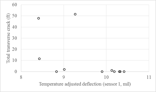
1 ft = 0.305 m.
1 mil = 25.4 microns.

Figure 85. Graph. Temperature-adjusted peak deflection at sensor 1 versus transverse cracking for SHRP test section 010101, F1.

Backcalculation of Pavement Layer Resilient Moduli Values

The measured and/or temperature-adjusted pavement deflection data, along with layer thickness and Poisson’s ratio, can be used to backcalculate the pavement layer moduli (M_R) values. Such values are useful in the design of pavement rehabilitation treatments. To further develop and verify the temperature adjustment procedures described previously, the deflection data from a few test sections were used to backcalculate the layer M_R values. The data used were from SHRP test sections 010101, 081053, 271028, and 351112. A partial record of the inventory data for the test sections used in this analysis are listed in table 108.

The MICHBACK software package, developed at Michigan State University, was used in the analyses to backcalculate pavement layer M_R values. MICHBACK uses the Chevronx computer program (a five-layer elastic program) as the forward engine to calculate the pavement deflections for a given set of layer moduli, Poisson ratios, layer thicknesses, and load magnitude. The MICHBACK program uses a modified Newtonian algorithm to calculate a gradient matrix by incrementing the estimated layer modulus values and calculating the differences between the measured and the calculated pavement deflection in three consecutive cycles. When the convergence criteria (specified by the program user) are satisfied, the iteration process stops, and the final set of backcalculated layer moduli are recorded.⁽⁸³⁾ In this study, the following convergence criteria were used:

• Modulus tolerance: Maximum modulus tolerance (the difference between two successive backcalculated modulus values) of 1 percent.
  
  
• Root mean square (RMS) error: Maximum RMS error tolerance (the square root of the sum of squared errors between measured and calculated deflections) of 5 percent.

The pavement layers were assigned the following Poisson’s ratio values:

• AC—0.35.
  
  
• Granular base—0.40.
  
  
• Roadbed soil—0.45.

Note that the aggregate base and sand subbase layers were combined into a singular base layer. This was done to improve the accuracy of the backcalculation.

The results of the backcalculation are listed in table 113. Note that for each location, three or four tests were performed during a 1-day period. Also note that the first set of four tests was conducted at point location 114.3, the next four at point location 91.4, and the third four was the average for the entire test section. The first set of three tests was conducted at point location 30.5, the next three at point location 7.6, and the final three at point location 7.6. The pavement surface temperature varied throughout each day of testing by as much as 82 ºF (28 ºC). Hence, the AC layer M_R value varied throughout the day. Higher temperature corresponded to softer asphalt binder and lower M_R. There were also some changes in the base layer M_R values and minimal changes in the roadbed soil M_R values. The changes in AC layer M_R are shown as a function of pavement surface temperature for the analysis using both the measured and temperature-adjusted deflection data in figure 86 through figure 89. The data in the figures indicate that in general the AC layer M_R values decreased with increasing temperature based on the measured deflection, while the values based on the temperature-adjusted deflection were opposite. Note that the two curves generally cross near the reference temperature of 70 °F (21ºC). This finding supports the use of the equation in figure 72 and indicates that the AC layer modulus values could be determined from the model of the backcalculated moduli values based on the measured or temperature-adjusted data by selecting the value at 70 °F (21 ºC).

Table 113. Backcalculated resilient modulus values.

ºF = 1.8 × ºC + 32.
1 psi = 6.895 kPa.

Figure 86. Graph. AC layer M_R values versus pavement surface temperature for SHRP test section 010101.

ºF = 1.8 × ºC + 32.
1 psi = 6.895 kPa

Figure 87. Graph. AC layer M_R values versus pavement surface temperature for SHRP test section 081053.

ºF = 1.8 × ºC + 32.
1 psi = 6.895 kPa.

Figure 88. Graph. AC layer M_R values versus pavement surface temperature for SHRP test section 271028.

ºF = 1.8 × ºC + 32.
1 psi = 6.895 kPa.

Figure 89. Graph. AC layer M_R values versus pavement surface temperature for SHRP test section 351112.

The backcalculated M_R values were further evaluated by plotting the results based on measured data versus those based on temperature-adjusted data, as shown in figure 90 and figure 91. The data in the figures indicate that minimal bias existed in the procedure for temperature adjustment across the various testing temperatures. Some data were reduced, and some data were increased following adjustment based on temperature (i.e., temperature adjustment did not consistently lead to increases or decreases in backcalculated M_R values).

ºF = 1.8 × ºC + 32.
1 psi = 6.895 kPa.

Figure 90. Graph. AC layer M_R values from measured and temperature-adjusted deflection data.

1 psi = 6.895 kPa.

Figure 91. Graph. Base and roadbed soil layer M_R values from measured and temperature-adjusted deflection data.

Although the backcalculation of pavement layer M_R values using temperature-adjusted pavement deflection was shown to work, many pavement engineers recommend performing backcalculation on measured data and then adjusting the results. This is because temperature adjustment in general is not exact, and it can introduce error. Such error can be magnified when the backcalculation routine is performed. Hence, making the adjustment at the end is preferred by many.

Rigid Pavement Deflection Versus Time

The measured rigid pavement deflections were evaluated over time using the following steps:

• Step 1: The deflection, treatment, and inventory data were downloaded from the LTPP Standard Data Release 28.0 for each of the SPS-2 test sections listed in table 114.

The data were sorted based on the applied load and the various test locations within the lane. Drop height 2 simulated the application of a 9,000-lbf (40-kN) half single axle load and was selected for analyses. The tests performed at the middle lane at mid-panel location (J1) were selected for individual analyses. All data from other test loads and locations were not included in the analyses.

Table 114. LTPP SPS-2 partial inventory data.

• Step 2: On any particular test day, a series of four tests were conducted at drop height 2 for each of about 10 locations along the test section. The deflection tests conducted on a test section in each specific testing day were averaged to simulate the data that would be collected by a State transportation department (one test per section). Deflection data collected after the application of a treatment were not included in the analyses.
  
  
• Step 3: The measured deflection data were plotted against time as shown in figure 92 for sensor1. The data in the figure indicate that the deflection increased and then decreased, and overall decreased over the 4-year period of data collection, with values of about 4.33to 5.91 to 3.94 inches (110 to 150 to 100 microns). Localized fluctuations occurred due to moisture conditions at the time of testing and instrument and measurement variability.

1 mil = 25.4 microns.

Figure 92. Graph. Measured peak deflection at sensor 1 versus time for SHRP test section 100201, J1.

• Step 4: The measured deflection versus time plots were visually evaluated, and the results are summarized in table 115. The data in the table indicate that 45 percent of the test sections showed increasing deflection over time, 27 percent showed more or less consistent deflection, and 27 percent showed decreasing deflection over time. Consequently, the time-dependent deflection measured over a 4-year period cannot be used as an indication of pavement deterioration or pavement distress.

Table 115. Summary of deflection for sensor 1 versus time trend descriptions for LTPPSPS-2.

• Step 5: Although the deflection data did not show a consistent trend over time, the data were further investigated by comparing the deflection with the pavement condition and distress data measured over the same time period. Because deflection, IRI, faulting, and cracking data were not collected at the same time, the data were grouped and taken as a calendar year average for comparison. Examples of such comparisons are shown in figure 93 through figure 96. The data in the figures indicate there was no trend in relationship between deflection and pavement condition or distress. Similar results were found for the other test sections.

1 inch/mi = 0.0158 m/km.
1 mil = 25.4 microns.

Figure 93. Graph. Measured peak deflection at sensor 1 versus IRI for SHRP test section 100201, J1.

1 inch = 25.4 mm.
1 mil = 25.4 microns.

Figure 94. Graph. Measured peak deflection at sensor 1 versus faulting for SHRP test section 100201, J1.

1 ft = 0.305 m.
1 mil = 25.4 microns.

Figure 95. Graph. Measured peak deflection at sensor 1 versus longitudinal cracking for SHRP test section 100201, J1.

1 ft = 0.305 m.
1 mil = 25.4 microns.

Figure 96. Graph. Measured peak deflection at sensor 1 versus transverse cracking for SHRP test section 100201, J1.

The pavement deflection data could be used to estimate the pavement response to load and for the design of pavement treatments, etc. The LTPP rigid pavement deflection data did not support the use of deflection as an indicator of impending surface distress. Therefore, deflection could not be used in this study as a component of RFP or RSP.

Rigid Pavement LTE Versus Time

The LTEs calculated based on FWD testing were evaluated over time using the following steps:

• Step 1: The LTE, treatment, and inventory data were downloaded from the LTPP Standard Data Release 28.0 for each of the SPS-2 test sections listed in table 114.
  
  
• Step 2: The data were sorted based on the applied load and the various test locations within the lane. Drop height 2 simulated the application of a 9,000-lbf (40-kN) half single axle load and was selected for analyses. The tests performed in the outer wheelpath at joint approach locations (J4) were selected for individual analyses. All data from other test loads and locations were not included in the analyses.
  
  
• Step 3: On any particular test day, a series of four tests were conducted at drop height 2 for each of about 10 locations along the test section. The various LTE tests conducted on a test section in each specific testing day were averaged to simulate the data that would be collected by a State transportation department (only one test per section). LTE data collected after the application of a treatment were not included in the analyses.
  
  
• Step 4: The LTE data were then plotted as a function of time. An example of such a plot is provided in figure 97. The data in the figure indicate that the LTE generally increased over the 4-year period of data collection, ranging from about 88 to 98 percent. Some localized fluctuations occurred as a result of the moisture conditions at the time of testing along with instrument and measurement variability.

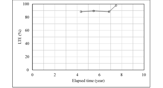
Figure 97. Graph. LTE versus time for SHRP test section 100201, J4.

• Step 5: The LTE versus time plots were visually evaluated and the results are summarized in table 116. The data in the table indicate that 21 percent of the test sections showed increases in the LTE over time, 30 percent showed consistent LTE, and 48percent showed decreases in the LTE over time. Once again, statistically speaking, the LTPP LTE data could not be used as an indicator of pavement distress or deterioration.

Table 116. Summary of LTE versus time trend descriptions.

• Step 6: Although the LTE data did not show a consistent trend over time, the data were further investigated by comparing LTE with the condition and distress data measured over the same time period. Because the LTE, IRI, faulting, and cracking data were not collected at the same time, the data were grouped and taken as a calendar year average for comparison purposes. Examples of such comparisons are shown in figure 98 through figure 101. The data in the figures indicate that there was no trend in the relationship between LTE and pavement condition or distress. Similar results were found for the other test sections.

1 inch/mi = 0.0158 m/km.

Figure 98. Graph. LTE versus IRI for SHRP test section 100201, J4.

1 inch = 25.4 mm.

Figure 99. Graph. LTE versus faulting for SHRP test section 100201, J4.

1 ft = 0.305 m.

Figure 100. Graph. LTE versus longitudinal cracking for SHRP test section 100201, J4.

1 ft = 0.305 m.

Figure 101. Graph. LTE versus transverse cracking for SHRP test section 100201, J4.

SUMMARY, CONCLUSIONS, AND RECOMMENDATIONS

This chapter presented the results of the analyses of the measured flexible and rigid pavement deflections and the LTE data. The main objective of the analyses was to determine whether pavement deflections and LTE data could be incorporated into the RFP and RSP algorithms.

It was envisioned that measured pavement deflections and/or LTE data would be correlated with pavement condition or distress, and hence, they could be used as an early warning of pending deterioration before it became visible on the pavement surface.

For flexible pavements, the measured pavement deflections were a function of the pavement temperatures. Therefore, the accuracy of the existing temperature adjustment methods were reviewed and scrutinized using the measured LTPP deflection data. Based on the results, a new global temperature adjustment methodology was developed that could be applied to all deflection sensors and all climatic regions.

Based on the results of the analyses, the following conclusions and recommendations were drawn:

• The LTPP deflection data collected for the SMP test sections did not support the use of the AI deflection temperature adjustment procedure. The equation in figure 72 was developed to more accurately adjust the measured deflection based on the asphalt surface temperature. It is recommended that the equation in figure 72 be used to adjust the measured flexible pavement deflections based on the measured pavement surface temperature.
  
  
• The LTPP deflection data collected for the SMP test sections did not support the inclusion of the deflection data in the RFP and RSP algorithms. It is recommended that the deflection data for flexible pavement be excluded from the RFP and RSP algorithms for the LTPP data.
  
  
• The LTPP deflection data collected for the SMP test sections did not correlate with the measured pavement condition and distress data. It is recommended that the flexible pavement deflection data not be used as an indication of impending pavement distress.
  
  
• The backcalculated AC layer modulus values of the selected LTPP test sections were dependent on the pavement surface temperature. To estimate the AC modulus at the standard temperature of 21 ºC, two procedures are recommended:
  
  
  • Adjust the measured deflection data to 21 ºC using the equation in figure 72 and then backcalculate the layer moduli.
    
    
  • During 1 day, conduct a minimum of three FWD tests and measure the pavement deflection at various times. Two FWD tests should be conducted at pavement temperatures below or above 70 °F (21 ºC) and the third test on the other side of 70°F (21 ºC). Backcalculate the AC modulus value for each of the three FWD tests. Plot the modulus as a function of the measured pavement temperature. From the graph, estimate the AC modulus at 70 °F (21 ºC).
    
    
• The LTPP deflection and LTE data collected for the SPS-2 test sections in Arizona, Colorado, Delaware, and Michigan did not support modeling of the data as a function of time. It is recommended that the deflection and LTE data for rigid pavement be excluded from the RFP and RSP algorithms.
  
  
• The LTPP deflection and LTE data collected for the SPS-2 test sections in Arizona, Colorado, Delaware, and Michigan did not support the correlation of deflection or LTE data with the measured pavement condition and distress data. It is recommended that the deflection and LTE data for rigid pavement not be used as indication of impending distress.
  
  
• It is further recommended that, for new LTPP experiments, the deflection data should be collected over a longer period of time (such as 10 to 20 years), and deflection data should be measured before and after treatments are applied.
  
  
• It is recommended that further research should be conducted to allow the incorporation of deflection data into the RFP and RSP algorithms. An early indicator of impending distress could prove to be very helpful to State transportation departments to allow them to treat the pavement before surface distress manifestation. In this study, although no relationships could be established based on the LTPP deflection data, future research could uncover such relationships.