U.S. Department of Transportation
Federal Highway Administration
1200 New Jersey Avenue, SE
Washington, DC 20590
202-366-4000
Federal Highway Administration Research and Technology
Coordinating, Developing, and Delivering Highway Transportation Innovations
| REPORT |
| This report is an archived publication and may contain dated technical, contact, and link information |
|
| Publication Number: FHWA-HRT-17-020 Date: February 2017 |
Publication Number: FHWA-HRT-17-020 Date: February 2017 |
The specimens were analyzed according to the level 3 design procedures outlined in AASHTO BDS to attain the LSS range. This design philosophy is based on the International Institute of Welding (IIW) document entitled Recommendations for Fatigue Design of Welded Joints and Components.(9) The LSS is defined via linear extrapolation of surfaces stress near the weld toe to the weld toe location. AASHTO BDS adopted the IIW coarse meshing option where the mesh size at the weld has element dimensions of approximately t by t, where t is the plate thickness. The IIW method requires extrapolating stresses from 0.5t and 1.5t distance away from the weld toe. It is further suggested that stresses are taken at mid-side nodes, suggesting that quadratic element formulations are used. This also requires two rows of elements, each t long, meshed on the extrapolated side of the weld toe. This is better shown in figure 13 where the geometry of the mid-plate thickness is shown. At the line defining the weld toe, two parallel lines are offset up the rib (generally in the Y direction) and across the deck plate (in the X direction). These parallel lines are offset by the thickness of the respective plates. Only one element width would be meshed between these parallel lines, and the mesh would be seeded across the width of the specimen (in the Z direction) such that the element width would be approximately t.
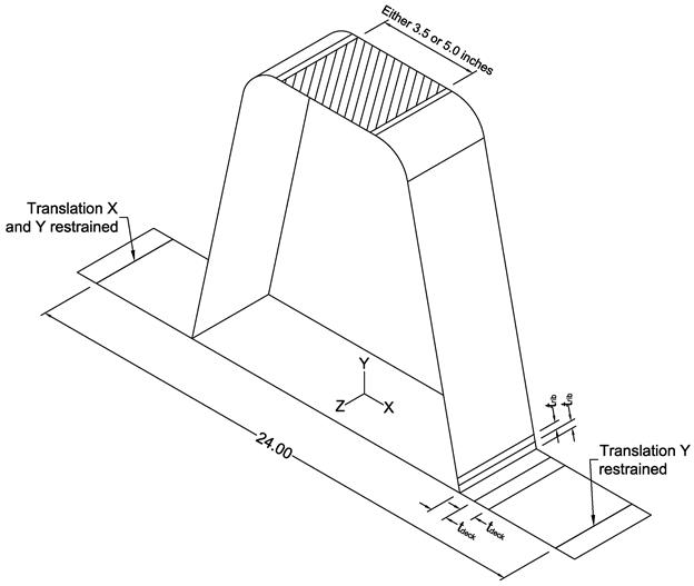
Units = Inches.
Figure 13. Illustration. Partitioning of specimen.
Since each lab used a different-sized thick plate washer to clamp the rib to the testing machine, each model was analyzed considering these two boundary conditions. Figure 13 shows a hatched area at the top of the rib. This hatched area was either 3.75 or 5 inches in the X direction for the specimens tested at VT and TFHRC, respectively. This area of the rib was modeled with a shell thickness of 2 inches to represent the added stiffness provided by the two thick plate washers. A unit point load was applied at the center of the hatched area to represent the applied load to the specimen. Because the specimens remained elastic, the results from this unit load analysis were multiplied by the applied load range to attain LSS ranges.
Finite element models were constructed with an analysis program capable of capturing nonlinear material and nonlinear geometric behavior; however, the models were fully elastic following the level 3 design procedure. A typical mesh is shown in figure 14. The mesh may appear discontinuous at the intersection of the rib and deck. With the restriction of approximately t by t element dimensions, it becomes difficult to attain a continuous mesh when there are large disparities in the plate thicknesses, such as this case, where the deck plate is over twice as thick as the rib plate. However, the analysis program has the capability of enforcing surface-based tie constraints between different parts. In this case, the rib and deck are modeled as individual parts and then assembled together with tie constraints to represent the weld. Tie constraints have no volume or mass; they merely enforce compatibility between two meshes. This enforces compatible displacements and rotations between the incompatible meshes through interpolation between node regions. Therefore, the rib and deck plates could be modeled with their respective t by t element dimensions within the same model.

Figure 14. Illustration. Meshed specimen.
As mentioned previously, only a unit load was modeled at the middle of the rib top. The resulting stress contours through a typical specimen is shown in figure 15 superimposed on the deflected shape. This contour plot shows the stresses at the element surfaces near the weld toe; these are in a direction perpendicular to the weld toe. The local structural extrapolation required interrogation of mid-side nodes at a distance of 0.5 and 1.5 plate thicknesses from the intersection. In AASHTO BDS, these are called the f0.5 and f1.5 stresess, and they should be in the direction perpendicular to the weld toe. The illustration shown in figure 16 is a zoomed-in view of figure 15 to just the weld region. Also shown by black dots are the mid-side nodes where the f0.5 and f1.5 stresses are taken for both the rib and deck plate. The model ignored the geometry of the weld as a simplification, and, because of this, the extrapolation was to the plate intersection, not the location of the theoretical weld toe. This was done for two reasons: (1) it was thought this would be a conservative assumption, and (2) all of the welds tested had quite a variation in weld geometry, so it would have been burdensome to model every specimen in lieu of just ignoring the weld.

Figure 15. Illustration. Membrane stress in specimen under unit load.

Figure 16. Illustration. Extrapolation points from rib and deck plate.
LSS results from all the models are shown in table 2 through table 4, respectively, for the types 1–3 specimen geometries. Because the models were based on unit loads, the f0.5 and f1.5 stresses reported are from the unit load. The flss stress is the actual LSS based on extrapolation. Because of the unit load analysis, all stresses are reported in units of ksi per kip of load. This was purposeful because in the fatigue analysis of the specimens, the flss value only had to be multiplied by the load range applied to the specimen to attain the total LSS range.
Table 2. LSSs from unit load for type 1 geometry.
| Test Lab | Location | f0.5 (ksi) |
f1.5 (ksi) |
flss (ksi) |
|---|---|---|---|---|
| TFHRC | Deck plate | 6.662 | 5.327 | 7.330 |
| Rib wall | 7.053 | 6.522 | 7.318 | |
| Weld root | 4.710 | 4.319 | 4.906 | |
| VT | Deck plate | 6.663 | 5.328 | 7.331 |
| Rib wall | 7.682 | 7.085 | 7.981 |
Table 3. LSSs from unit load for type 2 geometry.
| Location | f0.5 (ksi) |
f1.5 (ksi) |
flss (ksi) |
|---|---|---|---|
| Deck plate | 6.663 | 5.331 | 7.329 |
| Rib wall | 8.246 | 7.581 | 8.579 |
| Weld root | 5.906 | 5.378 | 6.170 |
Table 4. LSSs from unit load for type 3 geometry.
| Test Lab | Location | f0.5 (ksi) |
f1.5 (ksi) |
flss (ksi) |
|---|---|---|---|---|
| TFHRC | Deck plate | 9.734 | 7.692 | 10.755 |
| Rib wall | 11.035 | 10.174 | 11.466 | |
| VT | Deck plate | 9.733 | 7.692 | 10.754 |
| Rib wall | 11.457 | 10.547 | 11.912 |
Because of the boundary condition differences between the two labs, table 2 and table 4 report different flss values for each lab, as those rib geometries were tested at each lab. The type 2 geometry in table 3 was only tested at VT.
Finally, it can be noted that in table 2 and table 3, LSSs are also reported at the weld root. The LSS method was never intended for characterizing the stress state at a weld root. However, in this research, some specimens failed from the weld root, and, to plot those failures relative to all the other data, the LSS was extrapolated on the inside surface of the rib wall to represent the LSS of the weld root.

