U.S. Department of Transportation
Federal Highway Administration
1200 New Jersey Avenue, SE
Washington, DC 20590
202-366-4000
Federal Highway Administration Research and Technology
Coordinating, Developing, and Delivering Highway Transportation Innovations
| REPORT |
| This report is an archived publication and may contain dated technical, contact, and link information |
|
| Publication Number: FHWA-HRT-17-020 Date: February 2017 |
Publication Number: FHWA-HRT-17-020 Date: February 2017 |
Fatigue tests were performed on specimens consisting of differing geometries using two different load ratios. Furthermore, specimen weld dimensions varied from test to test. Thus, there were several possible sources of variation in fatigue resistance for the tested specimens. A statistical regression analysis was conducted to determine which factors and quantitative variables best explained the specimen‑to‑specimen variation in fatigue resistance. The primary objective of the regression analysis was to derive a parametric predictive model that could be used to calculate the fatigue resistance of welded orthotropic details similar to those examined in this study. Determining which test variables are most strongly correlated to fatigue performance allows the possibility of less uncertainty in the classification of the proper fatigue design category for welded orthotropic details. As mentioned previously, the fact that small specimens were used to obtain fatigue resistance data was not considered as part of the analysis. All analysis was conducted using the R statistical computing environment.(11)
Table 18 summarizes the observed dataset variables that were considered in the regression analysis. Of the 12 variables, 5 were factor variables (i.e., categorical variables), and 7 were continuous variables. The range column gives the set of possible values for each variable. The meanings of the weld dimension variables are illustrated in appendix B and appendix C.
Table 18. Statistical data variables.
| Variable | Type | Range |
|---|---|---|
| Load Ratio | Factor | {−1, 0} |
| Failure mode | Factor | {Deck, Rib, Root} |
| Geometry | Factor | {Type 1, Type 2, Type 3} |
| Laser welded | Factor | {Laser, Non-Laser} |
| Root gap opening | Factor | {Open, Closed} |
| Cycles | Continuous | ≥ 0 |
| Stress range | Continuous | ≥ 0 |
| d1 | Continuous | ≥ 0 |
| d2 | Continuous | [0,1] |
| d4 | Continuous | ≥ 0 |
| h | Continuous | ≥ 0 |
| t | Continuous | ≥ 0 |
With the exception of some of the laser-welded specimens, the dataset consisted of complete observations. As shown in appendix C, weld geometry measurements were available for only 10 of the laser welded specimens. One of the primary goals in building a predictive regression model was to uncover possible relationships between weld geometry and fatigue resistance. Thus, the laser-welded specimens without weld measurements were excluded from the regression analysis. While it is possible to impute values for the specimens without measurements in some way using the specimens for which measurements were available, this was avoided so as not to diminish any relationships between geometry and resistance.
The dataset originally consisted of 144 specimens after excluding runouts. Eliminating laser specimens without weld geometry measurements removed 28 specimens from the analysis dataset. In addition, specimens GM8‑3 and SA8‑9 were removed from the dataset for statistical analysis purposes after data preprocessing, leaving 114 specimens. The fatigue resistance of specimen GM8‑3 was significantly higher than for the remaining specimens with the same load ratio. Examination of the data in table 5 shows that this specimen was loaded at 20.16 ksi for 18,253,515 cycles prior to failure. This is the third-lowest stress range amongst all of the specimens tested from that series. The only two specimens with a lower stress range were runout specimens. It is likely that the loading conditions for specimen GM8‑3 were within the transition region in going from log‑linear S‑N behavior to infinite fatigue life behavior. As is the case with the runout specimens, banishing the specimen from the dataset results in more conservative fatigue resistance predictions.
It can be seen in table 6 that specimen SA8‑9 had a particularly low fatigue resistance relative to other specimens. Exploratory data analysis revealed that the weld dimension along the rib plate, h, was noticeably lower than the measured values for other specimens relative to the specimen rib thickness. It was suspected there may have been a transcription error with this specimen, and it was excluded from the dataset to prevent it from masking relationships. All plots and analysis moving forward in this chapter correspond to the dataset after removal of the aforementioned specimens.
The S‑N fatigue life model for welded steel bridge details implicitly assumes that there is a linear relationship in log‑log space between the number of cycles to failure and the applied stress range when the stress range is above some specified fatigue threshold. In non‑log space, this amounts to saying that the number of cycles to failure for a welded steel bridge detail is proportional to the stress range raised to some power. Thus, fatigue resistance can be thought of as a product of the underlying process parameters in non‑log space. The error component in this case can be assumed to be a positive multiplicative value as opposed to additive. With this in mind, the regression function used to model the experimental fatigue resistance coefficients in its most general non‑log form is shown in figure 34.

Figure 34. Equation. General regression function.
Where:
Ai = Fatigue resistance coefficient of the ith test specimen.
à = Base fatigue resistance coefficient (ksi3).
xij = Value of the jth predictor variable for the ith test specimen.
βj = Coefficient corresponding to the jth predictor variable.
εi = Random error component (> 0) for the ith test specimen.
Thus, the fatigue resistance coefficient was modeled as the product of some base resistance coefficient and a series of p modifiers that depend on the observed experimental variables. Taking the base10 log of both sides of the equation given in figure 34 gives the result shown in figure 35.

Figure 35. Equation. Linear regression function.
It is seen from the form of this equation that the regression function is a linear model in log‑space. The fatigue resistance coefficient for a test specimen was taken as the product of the number of cycles to failure and the cube of the calculated hot spot stress range as is consistent with the fatigue provisions for welded steel bridge details included in AASHTO BDS. Thus, it was implicitly assumed that the number of cycles to failure for a test specimen is inversely proportional to the cube of the corresponding stress range.
It should be noted that the value of the base fatigue resistance coefficient depends on relative factor levels should any factor variables be included as predictors in the model. Non‑reference factor variable levels were coded in standard non‑log space as either 1 if not applicable or 10 if applicable, corresponding to values of either 0 or 1, respectively, in the additive log‑space regression function of figure 35. Thus, the presence of a factor variable in the model amounts to increasing or decreasing the fatigue resistance coefficient by a specified constant multiplicative factor in standard space when applicable. Also, note that if the random error component follows a lognormal distribution, then the value in parentheses of the equation in figure 34 represents the conditional median value of the fatigue resistance coefficient given the specified values of the predictor variables.
Regression analysis involves determining the unknown model parameters for the chosen function that minimize some specified error criterion for the dataset that was used in the analysis or the training set. The average error of a fitted regression model corresponding to the training set observations will tend to be lower than the actual error that would be observed when using the model to predict a response for new and unseen observations that were not part of the training set. Thus, a different selection criterion other than training error is necessary to select a model that minimizes prediction error for unseen observations that were not part of the model fitting process.
For the fatigue resistance analysis, repeated tenfold cross‑validation was used as a means to select the optimal model that minimizes prediction error. Tenfold cross-validation involves randomly splitting the statistical dataset observations into 10 approximately equally sized subset splits. A candidate regression model is then fit 10 times to the data, leaving a different split out each time. The excluded split is used to estimate the prediction error of the candidate model. The cross‑validation errors for the model are then averaged over all splits. The average errors can be used to discriminate between different candidate models that were fit using different model parameters. Five tenfold repetitions were used in calculating cross‑validation errors for a total of 50 model fits corresponding to a given candidate regression model. The calculated average error for a specific training/test split was naively assumed to be independent of the average error calculated using some other split. In the case of standard linear regression, different candidate models correspond to models containing different combinations of the predictor variables.
Using standard least squares linear regression, the values of the predictor variable coefficients in the equation of figure 35 are determined by minimizing the sum of the squared model residuals over some training set of observations, given by the equation shown in figure 36.

Figure 36. Equation. Standard least squares regression error function.
The model-tuning parameter to be determined by cross‑validation in this case was the number of predictor variables to be included in the regression function. Table 19 lists the predictor variables considered in fitting the least squares model. For factor variables, the reference level used in the regression analysis is listed in parentheses in the “Type” column. The levels for each factor variable were given in table 18. Note that for the factor variable coding scheme used, the number of candidate predictors for a factor variable is always one less than the number of corresponding factor levels; as mentioned previously, the reference level given in parentheses is implicitly included as part of the base fatigue resistance coefficient of the regression function. Weld dimension predictor variables were normalized by the d4 dimension, which is strongly related to the thickness of the orthotropic rib plate. This was done so that the weld dimension variables would be independent of the overall structural geometry between different specimens. For example, one might expect that a 1/4-inch weld would experience different stress gradients in a structural configuration where the rib plate was 1 inch thick compared to a configuration where the rib plate was only 1/2 inch thick. The d3 dimension and the d5 dimension were excluded because they are linear combinations of the weld dimensions that are shown in the table and result in near perfect correlations with the other dimensions even after the log transformation.
Table 19. Standard regression predictor variables.
| Variable | Type |
|---|---|
| Load Ratio | Factor (−1) |
| Failure mode | Factor (Deck) |
| Geometry | Factor (Type 1) |
| Laser | Factor (Laser) |
| Gap | Factor (Closed) |
| d1/d4 | Continuous |
| d2/d4 | Continuous |
| h/d4 | Continuous |
| t/d4 | Continuous |
| (Failure mode):(d1/d4) | Factor-continuous interaction (Deck:d1/d4) |
| (Failure mode):(d2/d4) | Factor-continuous interaction (Deck:d2/d4) |
| (Failure mode):(h/d4) | Factor-continuous interaction (Deck:h/d4) |
| (Failure mode):(t/d4) | Factor-continuous interaction (Deck:t/d4) |
| (Load Ratio):(d1/d4) | Factor-continuous interaction (Load ratio = −1:d1/d4) |
| (Load Ratio):(d2/d4) | Factor-continuous interaction (Load ratio = −1:d2/d4) |
| (Load Ratio):(h/d4) | Factor-continuous interaction (Load ratio = −1:h/d4) |
| (Load Ratio):(t/d4) | Factor-continuous interaction (Load Ratio = −1:t/d4) |
Even though deck plate thickness did vary in the testing matrix, this was not exclusively considered in the regression because it was inherently coupled to the stress range calculation.
In addition to the factor variables and normalized weld dimensions, interaction variables between each normalized weld dimension together with the failure mode and load ratio were considered. This was done to account for the possibility that one weld dimension may be of greater importance in the presence of a particular failure mode or load ratio in comparison to other dimensions. Including such an interaction in the model would result in a change of the weld dimension exponent as shown in the equation of figure 34 given the occurrence of the particular failure mode or load ratio under consideration in the interaction.
Forward stepwise selection with a slight modification to satisfy the principle of hierarchy was used to select the best model for each given model size and a given training/test cross‑validation split. The principle of hierarchy specifies that when an interaction term is included in a regression model, it should also be the case that the main effects of the interaction are included in the model to preserve the intended meaning of the interaction. Thus, if it were determined by forward selection for a given model size that the best model included an interaction term, a check was made to insure that the main effect terms were already included in the model. If this was not the case, the next best model of the intended size was selected, and the check repeated until the principle of hierarchy was satisfied.
Figure 37 shows a plot of the average cross‑validation mean square errors (MSEs) as determined by the model fitting procedure. The error bars in the plot represent one standard error above and below the mean cross‑validation error. It is likely that the standard errors shown are larger in reality because of the implicit assumption of independence in the calculation. The zero variable model, or null model, corresponds to the case where only the base fatigue resistance coefficient is included in the regression function. This is equivalent to predicting the value of the fatigue resistance coefficient for a test specimen using the geometric mean of all observed resistance coefficients used to fit the model.
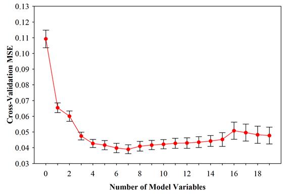
Figure 37. Graph. Standard regression cross-validation error.
The final model predictor variable coefficients in log‑space found using the aforementioned forward selection process applied to the full statistical dataset are given in table 20. The lowest cross‑validation error occurs when seven predictor variables are included in the model, not including the base fatigue resistance coefficient. Thus only models with seven variables or less are shown in the table. Also shown are the average cross‑validation MSEs together with the corresponding standard errors for the given number of variables used. While a model with seven predictor variables results in the lowest cross‑validation error, it can be seen that the cross‑validation error for a model containing four predictor variables falls within the standard error bounds for the seven variable model. Thus it was decided to use the less complex regression function containing three predictor variables as the final selected predictive model determined using standard regression. As can be seen in table 20, the four most influential predictors ranked in the order that they enter the model are load ratio, weld leg length along the deck plate, weld root failure, and weld penetration. The four‑variable model can be expressed as shown in figure 38.
Table 20. Final model regression coefficients by forward selection.
| Model Variables |
Cross- Validation MSE |
Standard Error of MSE |
à | Load Ratio = 0a |
d1/d4 | Weld Root Failureb |
d2/d4 | Root Failure: d1/d4b |
Rib Failure |
Rib Failure: d1/d4b |
|---|---|---|---|---|---|---|---|---|---|---|
| 0 | 0.109 | 0.00561 | 10.6 | NA | NA | NA | NA | NA | NA | NA |
| 1 | 0.0654 | 0.00308 | 10.7 | −0.447 | NA | NA | NA | NA | NA | NA |
| 2 | 0.0601 | 0.00327 | 10.8 | −0.450 | 0.661 | NA | NA | NA | NA | NA |
| 3 | 0.0475 | 0.00247 | 10.9 | −0.524 | 0.884 | −0.356 | NA | NA | NA | NA |
| 4 | 0.0427 | 0.00247 | 11.2 | −0.513 | 1.44 | −0.414 | 0.960 | NA | NA | NA |
| 5 | 0.0417 | 0.00257 | 11.2 | −0.514 | 1.51 | −0.416 | 1.02 | −3.12 | NA | NA |
| 6 | 0.0399 | 0.00294 | 11.2 | −0.495 | 1.42 | −0.382 | 0.969 | −3.04 | 0.118 | NA |
| 7 | 0.0390 | 0.00297 | 11.2 | −0.494 | 1.476 | −0.389 | −0.985 | −3.09 | 0.0762 | −1.934 |
| aà value already includes the reference level of Load Ratio = −1 as shown in table 19. bà value already includes the reference level of failure mode = deck as shown in table 19. NA = Not applicable. |
||||||||||
![]()
Figure 38. Equation. Least squares regression final predictive model.
Where:
α1 = 1 for tension‑only loading, 0 for load reversals.
α2 = 1 for weld root failure, 0 otherwise.
After further simplification, the least squares regression final predictive model is shown in figure 39.
![]()
Figure 39. Equation. Simplified least squares regression final predictive model.
The model specifies that full load reversals (load ratio = −1) correspond to fatigue resistances in the test specimens approximately three times greater in an average sense than tension‑only specimens (load ratio = 0) assuming that other variables remain constant. It is also seen that there is a reduced fatigue resistance coefficient for weld root failures in comparison to other failure modes. Note that the model as shown is somewhat deceptive in this regard as a result of the fact that weld root failures occurred only in the presence of load reversals, so the two reduction factors in the model do not apply simultaneously for any of the specimens tested. Finally, it can be seen that the fatigue resistance is given as a function of the d1 weld dimension as well as weld penetration. For both variables, there is positive correlation with fatigue resistance. However, it should be noted that the d1 dimension has a higher exponent and is generally not restricted to values less than or equal to 1 as is the weld penetration. Thus, for the experimental specimens, the d1 dimension is a more influential predictor of fatigue resistance than is the weld penetration. Furthermore, as the normalized d1 dimension increases, the weld penetration generally tends to decrease. Thus, it makes sense to specify design requirements for the weld leg dimension.
A normal probability plot of the deleted residuals for the final model fit is shown in figure 40. The residuals were externally studentized and segregated by load ratio: squares for R = −1 and circles for R = 0. It can be seen that the residuals for the four‑variable model exhibit some right skewness with a mean approximately equal to zero. It is also seen that the tails of the residual distribution are dominated by specimens that were subjected to load reversals. The ramifications of the residual distribution in deriving design guidelines are discussed in the next section.
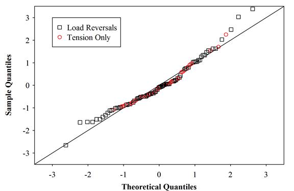
Figure 40. Graph. Normal probability plot of standard regression studentized residuals.
It was shown in figure 40 that the standard regression model residuals exhibit right skewness in log‑space. Figure 41 shows a histogram of the final fitted model residuals. Also shown on the plot are two different continuous normal distributions. The solid line distribution illustrates a normal distribution with location parameter equal to zero and scale parameter equal to the standard deviation of the fitted model residuals. As mentioned previously, the expected value of the MSE as calculated on the training set potentially gives an overly optimistic estimate for the actual error that would be observed when using the model to predict values for new observations. Thus, for design purposes, it is prudent to use a larger-scale parameter than is given by the standard deviation of the model residuals. The dashed line normal distribution shown in figure 41 is the distribution obtained when using the cross‑validation MSE to calculate the scale parameter. The tails of the distribution are larger than in the previous case. While the distribution does not precisely capture the small amount of skewness in the residual distribution, the tails of the distribution should provide a sufficient lower bound estimate for design purposes. Furthermore, if design guidelines are derived assuming a zero load ratio, most of the extreme residuals shown in the histogram become irrelevant, as was illustrated in figure 40. Thus, for design purposes, model predictions were assumed to have a lognormal distribution as represented by the green dashed line curve in figure 41 and a zero load ratio. The assumption of a zero load ratio will become clear in the derivations that follow.
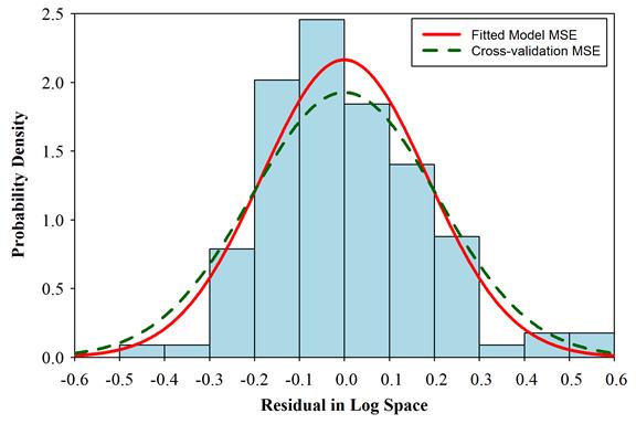
Figure 41. Histogram. Distribution of model residuals.
As is consistent with current fatigue design practice, a lower bound fatigue resistance for the experimental specimens can be expressed as the resistance corresponding to two standard deviations below the mean in log‑space. The cross‑validation standard deviation estimate (square root of the MSE) for the standard regression model was 0.207 in log‑space. Using this as an estimate of the true prediction error of fatigue resistance for the standard regression model gives for a design resistance coefficient as shown in figure 42.
![]()
Figure 42. Equation. Design fatigue resistance coefficient.
All variables in the equation are as defined for the equation in figure 38. As mentioned previously, it can be conservatively assumed for design purposes that the load ratio will be equivalent to the worst case, tension‑only load ratio loading. Revising the equation to account for this assumption and reverting out of log‑space gives the result shown in figure 43.
![]()
Figure 43. Equation. Simplified design fatigue resistance coefficient.
Regarding the occurrence of weld root failures, examination of the statistical dataset shows
the following:
Implicit in the inequality is the assumption of a zero load ratio, therefore it would be conservative to simply use the inequality of figure 44 with the weld root term eliminated. The second observation can be used as a basis for a fabrication guideline specifying that rib‑to‑deck welds be fabricated with closed root gaps in the welded condition. A final design inequality is shown in figure 44.
![]()
Figure 44. Equation. Design weld-dimension inequality.
There is discretion to choose a value for AD, though based on the presentation in figure 19 and figure 20, categories B or C would be most prudent. However, as the first term in figure 44 has a denominator of 187e08 ksi3 indicates the fitted model for design is halfway between category B (120e08 ksi3) and category A (250e08 ksi3). For the sake for further presentation of the design inequality, the first term in figure 44 can be represented by a constant, k, and results in the equation shown in figure 45.
![]()
Figure 45. Equation. Final design weld-dimension inequality.
The value of the constant, k, in the inequality is given in table 21 for fatigue design categories A–C.
Table 21. Weld leg design coefficient.
| Design Category | k |
|---|---|
| A | 1.35 |
| B | 0.630 |
| C | 0.222 |
Figure 46 graphically illustrates the experimental data and the derived weld design inequality of figure 45. The data are plotted with the weld penetration (d2/d4) on the y‑axis, and the normalized d1‑dimension is plotted on the x‑axis. The dashed lines represent the boundaries for fatigue design by category as given by the weld design inequality. The sizes of the plotted points are representative of the measured fatigue resistance coefficients as specified in the corresponding legends. As per the equation in figure 39, the fatigue resistances should increase in moving up and to the right of the graph, although the relationship gradients are not shown. It is noted that the inequality lines appear to be conservative as would be expected, considering the manner in which the inequality was derived. It is noted further that had load reversals been considered as part of the derivation, the inequality lines would move down and to the left of the plot. This should be taken into consideration when viewing the open markers that represent the tests where load reversals occurred.
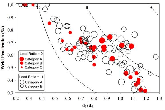
Figure 46. Scatterplot. Weld design inequality.
Because d1 only defines one dimension of the weld, it is also helpful to understand the range of h dimensions used in the experimental specimen pool to better define further geometric restrictions. Figure 47 shows a histogram of the h‑to‑d1 ratios for the experimental specimens tested. As can be seen, the majority of the ratios for the experimental specimens were between 0.5 and 2.0. To insure that the inequality of figure 45 is not used in designing weld geometries that are far removed from the geometries for the specimens from which the inequality was derived, the leg dimension along the rib for new welds should be bounded by these ratios.
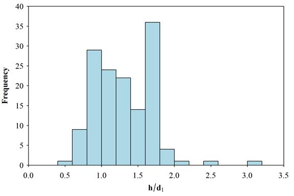
Figure 47. Histogram. Frequency of h‑to‑d1 ratio in experimental specimens.
Finally, the design parameter, k, used in the previous discussion provides leeway to selection of fatigue resistance to be categories C or B. Selecting one versus the other effectively changes minimum weld size and penetration per the design inequality. Considering the S-N plot shown in figure 22, category C would be a good candidate. Another reason to use category C is to avoid the conundrum of constant amplitude fatigue threshold (CAFT) with LSS analysis as the category C CAFT is 10 ksi. To illustrate the difference, figure 48 shows the variation in required weld sizes when using the category C design versus the category B design using the same rib and deck plate geometries with an assumed 60 percent penetration requirement. The design inequality was used to determine the required minimum d1 dimension, and then h dimensions of 0.6d1 and 2.0d1 were drawn to show the bounds. Therefore, the minimum weld is filled with a cross-hatch pattern and the maximum weld with a hatched pattern. While category B design would allow for use of higher stress ranges in the design model, this comes at the expense of a larger weld as shown in figure 48.
From the stance of this research, there should be no problem making the d1 dimension larger than output from the design inequality, though the largest d1/d4 ratio of all the specimens was approximately 1.30. This would be helpful because the minimum diagrammatic welds shown in figure 48 may not be welds that are efficient, or even feasible, and other criteria may control such as maintaining a throat dimension equal to the rib thickness. The design inequality allows the engineer to assume the rib-to-deck plate weld has category C resistance in design and allows them flexible detailing requirements in terms of weld penetration and deck plate leg length to ensure that category C resistance is delivered.
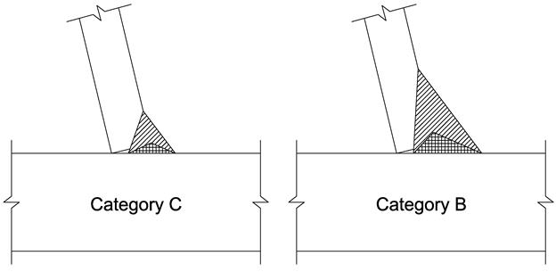
Figure 48. Illustration. Comparison of minimum weld dimensions for categories C or B fatigue design.