

Precast Bent System for High Seismic Regions: Laboratory Tests of Column-to-Drilled Shaft Socket Connections
MEASURED RESPONSE
This chapter reports the measured responses of specimens DS-1 and DS-2 during testing.
Moment-Drift Response
The moment-drift response is similar to the load-displacement response, but it differs slightly, because the moment includes components from both the vertical and lateral loads, whereas the load-displacement response includes only the horizontal load.
The moment at the base of column is given by the equation in figure 13.
Figure 13. Equation. Moment at the base of the column.
In figure 13:
Mc = the column moment at the base.
h1 = height from the column-shaft interface to the line of action of the lateral load.
h2= is the height from the interface to the top of column where the axial load, P, is applied by the Baldwin Universal Testing Machine.
V = applied lateral load.
Ffric = the friction force between the bearing and the sliding channel, and the greased steel-to-steel spherical element on bearing.
Δ1 = the lateral displacement at the location of the lateral load.
Δ2 = the lateral displacement at the top of column.
Δ3 = the lateral displacement at the top of transition, was taken approximately as lateral displacement at the first curvature rod (2 inches above the top of transition).
These parameters are illustrated in figure 14.
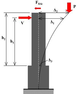
Figure 14. Diagram. Displacements and forces on test specimen.
In the absence of a measured value for Δ2, it was approximated by assuming the column rotated as a rigid body about its base, in which case the equations in figure 15 and 16 hold true.
Figure 15. Equation. Determination of axial load lateral displacement.
Figure 16. Equation. Moment at the base of the column.
It should be noted that the vertical load, P, contributed about one-third of the total moment at the maximum drift, and less than that at smaller drifts. Thus, any relative error in the approximation of creates a smaller relative error in the moment calculation.
Figure 17 shows the moment vs. drift ratio response of the test specimens DS-1 and DS-2. Because the columns used in these specimens were nominally identical to those used in spread footing specimens SF-1 and SF-2 by Haraldsson and SF-3 by Janes, results from those tests are shown for comparison.(10,14) The measured response of specimen DS-1 was similar to those of specimens SF-1 and SF-2. In all three cases, failure occurred by plastic hinging in the column, while the connection region in the foundation remained largely undamaged. However, in specimens DS-2 and SF-3, failure occurred in the connection region after some damage had first occurred in the column. This difference is apparent in the figures for those specimens, in which the strength decays with increasing drift more rapidly than is the case in SF-1, SF-2, and DS-1.
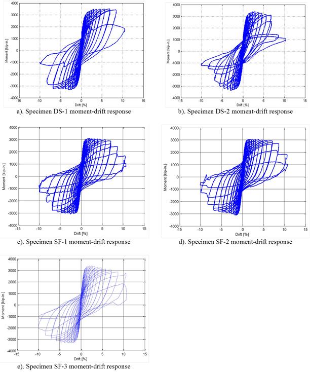
Figure 17. Graphs. Moment vs. drift ratio response.
In all cases, the peak moment occurred at about 2.5 to 3 percent drift ratio, and the moment first dropped below 80 percent of the peak value at about 8 percent drift, except in DS-2 where it occurred at about 7 percent drift; the response was very ductile. The similarity between the peak strengths in specimens SF-1, SF-2, and DS-1 was expected because the columns were nominally identical and the specimen strength was controlled by the column response. (The primary difference was the concrete strengths.)
As shown in table 6, the maximum moments at the interface were approximately 3,400 kip-in. in both specimens DS-1 and DS-2. The stiffness of the columns was measured at the force corresponding to the first yield of column reinforcement. It shows that DS-1 had nearly the same stiffness as DS-2.
Points of Interest |
DS-1 | DS-2 | ||
|---|---|---|---|---|
| North Direction | South Direction | North Direction | South Direction | |
Secant Stiffness at Initial Yield Moment (kip/in.) |
109 |
126 |
101 |
122 |
Maximum Column Interface Moment (kip-in.) |
-3,290 |
3,476 |
-3373 |
3,393 |
Drift Ratio at Maximum Column Interface Moment (%) |
-3.09 |
6.83 |
-2.96 |
2.90 |
80% of Maximum Column Interface Moment (kip-in.) |
-2,657 |
2,811 |
-2,293 |
2,337 |
Drift Ratio at 80% of Maximum Interface Column Moment (%) |
-8.27 |
8.15 |
-5.95 |
6.84 |
The columns were also stiffer in the south direction of loading, which was the direction in which they were first loaded. This behavior was observed for both specimens. The exact reason for this behavior is unknown, but it appears to be related to the level of cracking, which is likely to have been larger in the direction of second loading.
Failure is commonly defined at the point where the maximum moment is 80 percent of peak moment. In specimen DS-1, it occurred after 8.0 percent drift ratio and corresponded to the onset of buckling of the column longitudinal reinforcement. However, in specimen DS-2, it occurred at about 6.0 percent drift, when vertical and diagonal cracks had propagated throughout the transition region, and the spirals were at incipient fracture.
The lateral load, , used in the equations in figures 14 through 16, was corrected for friction in the sliding bearing using the recommendation proposed by Brown.(21) The test setup in the Baldwin Universal Testing Machine created frictional resistance in the system by two mechanisms: rotation between the greased steel-to-steel spherical element in the swivel head bearing and sliding between the bearing's top flat plate and the channel attached to the Baldwin head. The friction component in the channel was minimized by placing a silicon-greased Teflon sheet on the bearing where it slid against smooth stainless steel plates in the channel. This correction was done previously in research on accelerated bridge construction (ABC) at the University of Washington.(5,21) The rotational element in the bearing was also greased, but because it consists of two mating steel surfaces, the friction there is necessarily higher.
The correction model consists of a bilinear spring with a spring stiffness, k, of 60 kips/in., and has a maximum friction force, , of where is a calculated coefficient of friction and was taken as 0.016, and P is the target axial load (160 kips).(21) Therefore, the estimated maximum resistance of approximately 2.56 kips. This is approximately 5 percent of the maximum applied lateral load in both tests.
Effective Force
The effective force acting on the specimens was calculated by dividing the moment at the interface by the height from the interface to the line of action of the lateral load. The equation in figure 16 is divided by to obtain the equation in figure 18.
Figure 18. Equation. Effective lateral force.
In figure 19, the effective force is plotted against displacement for both specimens. The shapes of the curves are identical to the moment-drift responses, but they are expressed in terms of the effective force and displacement.
Table 7 summarizes the values of 100 percent and 80 percent of the maximum effective force (MEF) and the corresponding displacements.
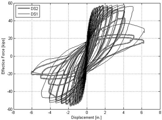
Figure 19. Graph. Effective force-displacement response.
| Points of Interest | DS-1 | DS-2 | ||
|---|---|---|---|---|
| North Direction | South Direction | North Direction | South Direction | |
Maximum Effective Force (kips) |
-54.8 |
57.9 |
-56.21 |
56.5 |
MEF Displacement (in.) |
-1.85 |
4.10 |
-1.80 |
1.74 |
80% of Maximum Effective Force (kips) |
-43.8 |
46.3 |
-45.0 |
45.2 |
80% of MEF Displacement (in.) |
-4.96 |
4.89 |
-3.57 |
4.02 |
Curvature
Average curvatures were computed from the measured displacement data at selected locations along the columns and shafts. They are reported here to show the distribution of bending deformations and to evaluate the contribution of bending to the total displacement.
In the columns, the curvatures were computed from local rotations, and near the bottom of the column, these were established by measuring the differential displacement on either side of the column of rods that were embedded horizontally into the concrete (see figure 20). These were referred to as "curvature rods." Higher up the column, where no curvature rods existed, the rotations were obtained from inclinometers attached to the column face.
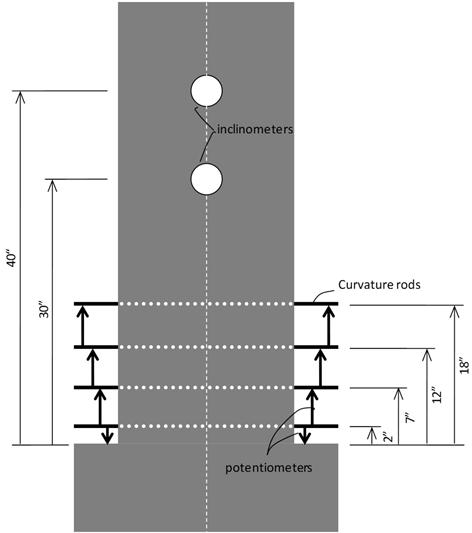
Figure 20. Diagram. Detailed curvature rods setup.
These methods were also used by Haraldsson and Janes.(10,14) Curvature rods were embedded in the column about 2, 7, 12, and 18 inches above the interface. The average curvatures between rods were plotted at the mid-point of those segments. The curvatures were calculated using the equation shown in figure 21.
Figure 21. Equation. Calculating curvature.
In figure 21:
φi = the calculated average curvature.
δi,N and δi,S = the relative displacement between rods on the north side and south side at particular height above the interface.
Li = the horizontal length between north and south potentiometers.
Hi = the height of each segment.
Above the rod position, the column average curvatures were obtained by the column average rotation difference between two inclinometers.
The shaft average curvatures were determined from the shaft rotation at selected locations (measured by the motion capture system). At each level, one marker was attached on each of the north, south, and west sides of the shaft. The rotations of the shaft were taken as the rotation of the plane defined by these three points.
Figure 22 shows the average column curvature versus height for selected drift ratios. The height was relative to the column-shaft interface.
The curvatures were plotted up to 6.8 percent drift. The curvature data at higher drift were not reliable because the spalling of concrete in the column in specimen DS-1 and in the top surface of the shaft in specimen DS-2 affected the potentiometers. The column curvature distribution was similar in both specimens until 3.0 percent drift. These curvatures were similar because, up to that drift, the majority of the displacement was in both cases provided by the column. The deformation was distributed over the column height, with the largest values at the bottom. The latter were caused by the formation of a significant crack at the column-shaft interface, which dominated the displacement measured by the potentiometers. The segment length at the bottom was also short (2 inches), and the average rotation measured included column rotation and bending rotation; thus, the computed curvature was relatively high. The concept of curvature is based on the existence of a continuous deformation field. In a cracked, discontinuous, medium, such as the concrete in the columns and shafts, the calculated curvature is not unique and depends on both the segment size and the locations of the cracks relative to the segment boundaries. Nonetheless, the distribution of computed curvature gives an overall sense of the distribution of bending deformations.
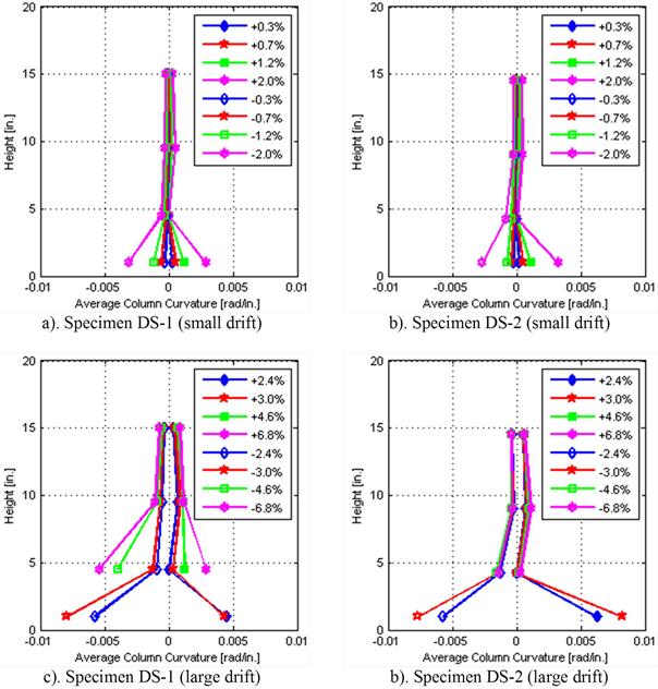
Figure 22. Graphs. Average column curvature (specimen DS-1 and DS-2).
At higher drift ratios (after 3.0 percent drift), because of the onset of spalling at the top of transition, the strain values at the bottom segment measured by potentiometers were unreliable; they are plotted in the figures. The column curvature distribution differed between the two specimens. In DS-1, the average curvature at 5 inches above the interface increased rapidly while it did not change in DS-2. That was consistent with the damage progression in two tests when spalling occurred in DS-1 and did not happened in DS-2. The bond stress between the column and shaft started degrading, and the shaft in specimen DS-2 started to deform significantly. Thus, at any given drift, the column curvature was smaller in specimen DS-2 than in specimen DS-1.
In DS-2, a method using three "Optotrak" markers was used to measure rotation in the column to compare with the result of using curvature rods. The column average curvature versus height for selected drift ratios are provided in figure 23. The results of column curvature distribution were quite similar by using Optotrak markers and curvature rods. The different curvatures at the bottom segment were unknown, but these values were unreliable, as explained previously.
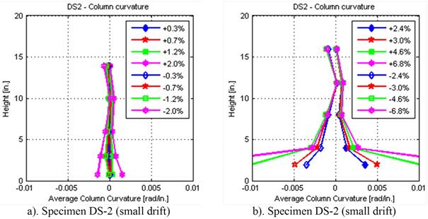
Figure 23. Graphs. Average column curvature (measured by Optotrak) in specimen DS-2.
The average shaft curvature versus height for selected drift ratios is shown in figure 24. The curvatures in the shafts were also distributed non-uniformly, with the largest values at the base. Such distribution reflects the existence of a flexural crack at the base. Each of the peaks of curvature corresponds to a horizontal crack position. Note that the scales on the column and shaft plots are different, and that the shaft curvatures were smaller by about an order of magnitude than the column curvatures.
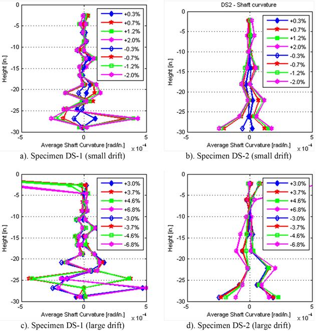
Figure 24. Graphs. Average shaft curvature for specimens DS-1 and DS-2.
Displacement
In the test specimens, the horizontal displacement at the top of the column depended on the deformations of the individual elements. To simplify discussion, those deformations are broken down into the following components, which are illustrated in figure 25.
- Shaft bending deformations. These are the curvatures of the shaft, and they depend on the elongation of one vertical face and the shortening of the opposite one. Curvature was measured by the three Optotrak markers attached to the shaft at the same level, using the motion capture system. At each level, one Optotrak marker was attached on each of the north, south, and west sides of the shaft. The rotations of the shaft were taken as the rotation of the plane defined by these three points. Then, the average curvature of segment was calculated by dividing the difference of rotation at the adjacent level to the segment's height.
- Shaft shear deformations. These deformations consist of pure shear deformations of the shaft. They were obtained by subtracting the shaft bending displacements from the total horizontal displacements. The total displacements were obtained from the horizontal displacements measured by the motion capture system (and verified by the string potentiometers). The bending displacements were obtained by integrating the rotations obtained from the shaft bending deformations.
- Column end rotations. The column can rotate as a rigid body, due to damage in the transition region of the shaft. These rotations were obtained from the bottom inclinometer attached to the column, and from the group of three Optotrak markers attached to the bottom of the column (2 inches above the interface).
- Column bending deformations. These deformations consist of the curvatures of the column. Rotations were measured at discrete locations up the column, and the average curvature was computed from the difference between rotations at adjacent locations. The rotations were obtained using inclinometers, curvature rod instruments, and Optotrak data.
- Column shear deformations. These consist of the pure shear deformations of the column. They were very small in both cases, and they were estimated by subtracting the total displacement to the displacement of components 1, 2, 3, and 4. This value would include error in this computation.
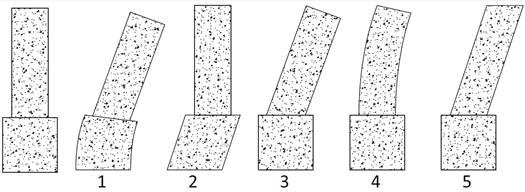
Figure 25. Illustration. Displacement types.
The displacements were calculated at the top of the column (60 inches above the interface). The shaft bending displacements were calculated by numerically integrating the shaft curvature over the height of the shaft. The shaft shear displacements were calculated by subtracting the shaft bending displacements at the top of the shaft from the total shaft displacement (using Optotrak measurements). The displacements due to column end rotation were calculated as the product of column height and the difference between the rotation of the column at 10 inches above the interface (measured by an inclinometer) and the rotation of shaft at the interface (measured by the Optotrak). The displacements due to column bending were calculated by numerically integrating of the column curvature. The column shear displacement and error of the instruments were calculated by subtracting the displacements due to shaft bending, shaft shear, column end rotation, and column bending from the displacement at the top of the column (as measured by a string potentiometer).
Vertical displacements were measured only by the Optotrak system. No values are presented here.
The method of measuring rotation of specimens using groups of three Optotrak markers was compared with the results obtained using the inclinometers to show the accuracy of this method. The comparison is shown in figures 26 and 27 for the results measured in specimen DS-2. The comparison shows that the Optotrak method and the inclinometers provided similar results.
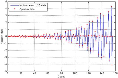
Figure 26. Graph. Rotation comparison at 10 inches above the interface position (specimen DS-2).
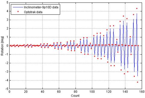
Figure 27. Graph. Rotation comparison at 18 inches above the interface position (specimen DS-2).
The displacement profiles of the shaft and column are plotted for specimens DS-1 and DS-2 in figure 28 and figure 29, respectively. The vertical axis represents the distance above the base of the shaft, while the horizontal axis is the displacement in inches. Note that the shaft was 30 inches high, and the height of the column, measured from the top of the shaft to the loading point, was 60 inches.
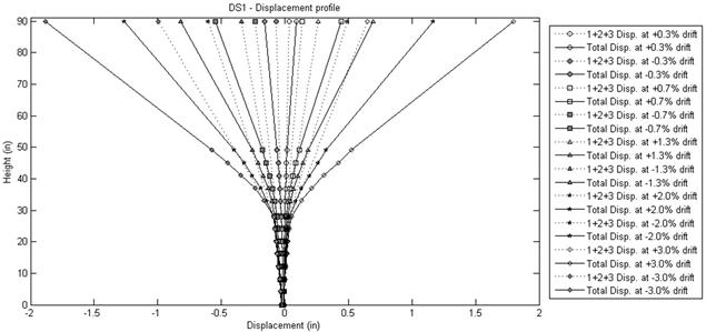
Figure 28. Graph. Specimen DS-1 displacement profile.
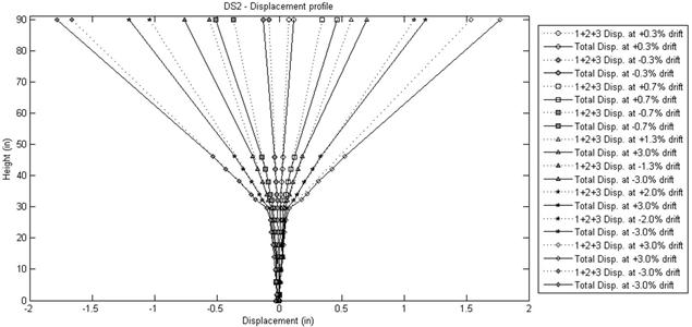
Figure 29. Graph. Specimen DS-2 displacement profile.
Profiles are given for the peak displacement in each cycle set, up to 3.0 percent drift. Separate curves are given for the positive and negative directions. For each load level, two curves are presented. The solid line represents the total displacement, while the dashed line represents the sum of the displacements due to components 1, 2, and 3 (shaft bending, shaft shear, and column base rotation). Components 1 and 2 may be thought of as shaft contributions to the overall displacement. Component 3 may be thought of as a column boundary condition contribution, which is nearly zero in Haraldsson's column-spread footing socket connection.(10) The differences between the dashed and solid lines for any load level, therefore, represent the displacement due to column bending and shear, or the column contributions to the total displacement. In all cases, the column shear component small compared with the column-bending component.
Up to 0.7 percent drift, the displacement profiles of specimens DS-1 and DS-2 were similar. The angle of dotted lines at the interface position corresponded to the appearance of column base rotation. Thus, the column base rotations were nearly zero because there was no angle at the interface position in the dotted lines.
However, after 0.7 percent drift, the behaviors of specimens DS-1 and DS-2 were different. Overall, the majority of the displacement in specimen DS-1 arose from column deformations, because a plastic hinge started to form in the column. By contrast, in specimen DS-2 the column deformations were small, and the column base rotations deformations dominated the behavior of the specimen.
The details of the response were as follows. In specimen DS-1, the column bending deformation kept increasing with each cycle up to 3.0 percent drift. This was suggested by the rapid increasing of the distance between solid lines and dotted lines at the top position at the same drift. On the other hand, in specimen DS-2, the column bending deformation decreased after 0.7 percent drift and was very small at 3.0 percent drift. The majority of the total displacement was attributable to column base rotation, which was 0.012 rad (1.2 percent drift) in DS-1 and 0.007 rad (0.7 percent drift) in DS-2. However, in DS-2, the percentage of the column base rotation contribution to total deformation was higher than in DS-1.
The contributions of the various displacement types are shown in figures 30 and 31. In specimen DS-2, after cycles to 7 percent drift, large vertical cracks appeared in the shaft. Thus, the data obtained from the Optotrak marker attached in the shaft were not reliable for calculating the curvature of the shaft. Therefore, the displacement of the shaft bending, column shear, and error were not reliable after 7 percent drift.
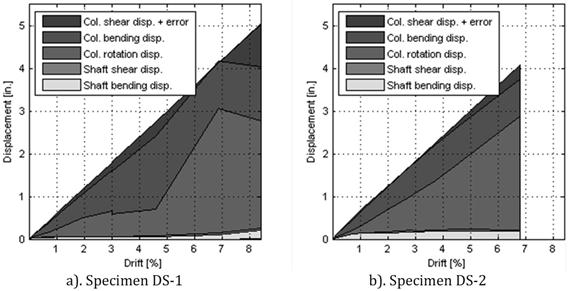
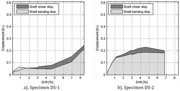
Figure 31. Graphs. Displacement-drift response of shaft (specimens DS-1 and DS-2).
As shown in the figures, the column bending deformations were higher in DS-1 than in DS-2 before decreasing at 7 percent drift. At this time, the column rebar was buckling and the concrete was crushed. In DS-2, the column bending deformation was smaller, and most of displacement at the top of the column was the column rotation displacement. In the shaft, the shaft shear deformation was similar in DS-1 and DS-2. However, the shaft bending in DS-2 was higher than in DS-1.
Strains in Column Reinforcing Bars
The longitudinal reinforcing bars in the column were gauged as shown in figure 32. Because they were configured symmetrically, only the East reinforcing bars were gauged. In both specimens, gauges were attached on the reinforcing bars in pairs at three locations: 0 in., 12 in. and 23 in. below the interface of the shaft and column.
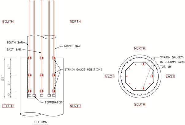
Figure 32. Diagrams. Column strain gauge positions.
Figure 33 shows the axial strain distributions (obtained by averaging the readings from each pair of gauges) over the height of the north, south, and east reinforcing bars at various drifts for DS-1 and DS-2. The strains were plotted up to 3 percent drift. Both specimens show similar strain profiles before yielding in the reinforcing bars. The plots show that the reinforcing bars in the north and south experienced alternate tension and compression as they were loaded cyclically, and they started to yield in tension at the column-shaft interface at 0.7 percent drift. The east reinforcing bars were located at the mid-depth of the column, so they experienced almost equal tension strains when the column was displaced to the north and south. They started to yield in tension at 1.2 percent drift.
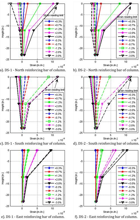
Figure 33. Graphs. Strain profiles in reinforcing bars of the column (until 3 percent drift).
At a location 12 inches below the interface, the bars started to yield at 2.0 percent drift in the north and south reinforcing bars, and at 3.0 percent drift in the east reinforcing bars in both specimens. After 3.0 percent drift, the tension strains began to exceed the measurement range of the data acquisition system, which was from -0.011 to +0.011 in./in. For real strains outside this range, the recorded value was +/- 0.011 in./in. When the real strain came back within the readable range, the correct value was again recorded.
The axial strains distributions after 3 percent drift are plotted in figure 34. Again, the recorded values are limited to the range +/- 0.11 in./in. They were plotted up to 8.4 percent drift, when the spiral in the column broke. At the next cycle, 10 percent drift, the reinforcing bars in the column broke, so no strain is presented.
The plots show that, after 3 percent drift, the strain distributions of specimens DS-1 and DS-2 were different. Consider first the bar strains at the interface. In both the north and south bars in specimen DS-2, and in the south bar in specimen DS-1, the bar experienced only modest compression strain (no more than -0.003 in./in.). This suggests that the concrete in the region was reasonably intact and was still carrying most of the compression force. By contrast, the north bar in specimen DS-1 experienced large compressive strains (to -0.009 in./in.) at 6.9 percent drift because the concrete had suffered significant damage and most of the force was being carried by the bars. However, by 8.4 percent drift, the column spiral has fractured and the bars had buckled, so the load they resisted and the strain they displayed were reduced.
At the bottom of the column, the bars in all cases never reached yield in tension. This suggests that the anchorage of the bars was being provided at least partly by bond. However, because the tension strain was close to yield, the anchor heads were clearly necessary. In specimen DS-2, the south bars exhibited high compression strains at drifts of 6.9 percent and above. These are believed to be caused by the column rocking on its edges after the resistance of the shaft had largely been lost. This can be seen in the figures illustrating the damage at the bottom of column of specimen DS-2 after testing (see appendix C).
The strain distributions in the east bars were also different between specimens DS-1 and DS-2. In specimen DS-1, the strain distribution was non-linear, suggesting that the moment decayed rapidly with depth. However, in specimen DS-2, after 4.6 percent drift, the strain distribution was linear. It suggests that there was no friction between the surface of column and the shaft, and that the moments were determined only by the horizontal forces at the top and vertical forces at the bottom of the transition region. It is also noticeable that the strains decreased after 4.6 percent drift. This is explained by the drop in load then, caused by the damage to the transition region of the shaft.
Figure 35 shows the cyclic effective force-strain relationships of the column reinforcing bars at the interface, 12 inches, and 23 inches below the interface in specimens DS-1 and DS-2. In each plot, the cyclic effective force-strain relationships were plotted for the north, south, and east reinforcing bars in blue, green, and purple, respectively, at the given depth.
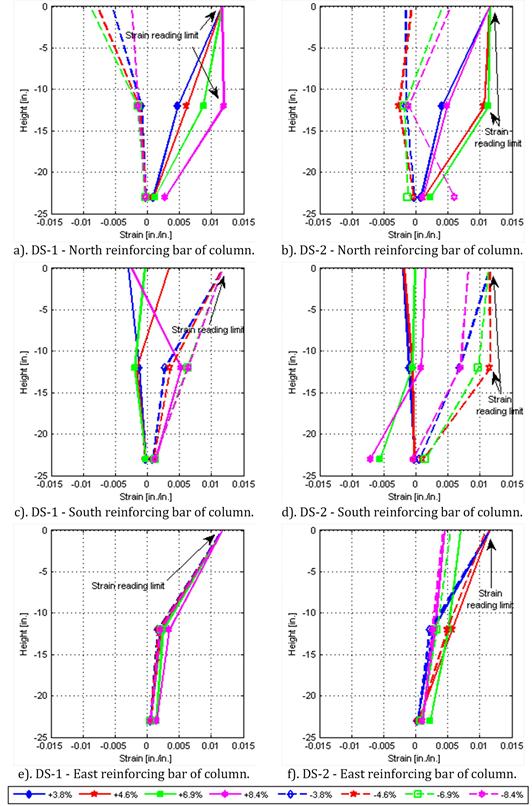
Figure 34. Graphs. Strain profiles in reinforcing bars of column (after 3 percent drift).
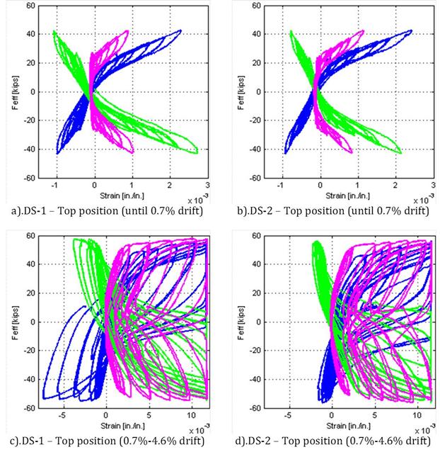
Figure 35. Graphs. Strain-effective force relationship of the column reinforcing bars.
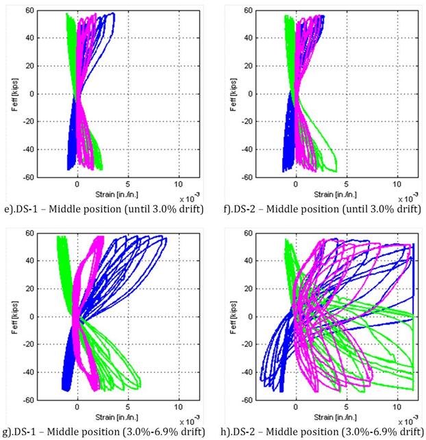
Figure 35. Graphs. Strain-effective force relationship of the column reinforcing bars, continued.
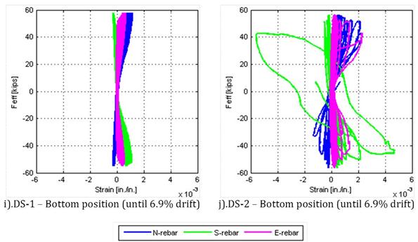
Figure 35. Graphs. Strain-effective force relationship of the column reinforcing bars, continued.
At the interface, up to 0.7 percent drift, the relationships in specimens DS-1 and DS-2 were similar. When the effective force reached 40 kips, the strains in the north, south, and east reinforcing bars were 2.25e-3, -1.0e-3, and 1.0e-3, respectively, in both specimens. This illustrated that the north and south reinforcing bars reached a yield point at 0.7 percent drift in both specimens. The relationships had a line of symmetry through effective force Feff = 0. At Feff = 0, all the strains in reinforcing bars were nearly zero. It suggested that the friction between the column surface and the shaft was still good. When the cyclic drift went from 0.7 percent to 4.6 percent, the relationships in DS-1 and DS-2 were different. As illustrated in the plots, the compression strain in the north and south reinforcing bars in specimen DS-1 were higher than in DS-2. This indicated that, at this time, the column concrete in DS-1 was crushed and more compression force was being carried by the bars. This contrasts with the behavior of specimen DS-2, where the column concrete was not crushed. During this period, the strains in the north, south, and east reinforcing bars in both specimens were not only non-zero when Feff = 0, but they also increased after each cycle.
At 12 inches below the column-shaft interface, up to 3.0 percent drift the relationships in both specimens were similar. It can be recognized that the friction between the column surface and the shaft were still good in both specimens because the strain values at Feff = 0 were nearly zero. When the drift increased from 3.0 percent to 6.9 percent, the relationships in DS-1 and DS-2 were different. In DS-1, the strain values when Feff = 0 were increased a little bit, which indicated that the friction was decreased but still good. That is because when the tension reinforcing bar strain dropped from two times the yield strain (0.004 in./in.) to zero, stress in that bar must be equal to compression yield strength (assume -60 ksi). At the same time, the compression reinforcing bar strain increased from about -0.001 in./.in to zero, so stress in that bar must be equal to half of the compression yield strength (assume -30 ksi). Therefore, when Feff = 0, the moment at this position by column reinforcing bars was not zero. Thus, friction moment must equal this value to equilibrate. The maximum values were 0.008, 0.006, and 0.002 in the north, south, and east reinforcing bars, respectively. The maximum effective forces remained about 60 kips. However, in DS-2, effective force decreased from about 50 kips to 35 kips. The strain values when Feff = 0 were not zero and increased after each cycle. This illustrated that the friction was lost. Therefore, most of flexure transferred to column. Thus, the strain in rebar increased dramatically over the reading capacity about 12e-3.
At 23 inches below the interface, the relationships were plotted from 0 percent to 6.9 percent drift. As shown, the reinforcing bars in specimen DS-1 remained elastic through the test. In specimen DS-2, they remained elastic up to 4.6 percent drift, during which the strain values were similar to those in specimen DS-1, but the bars yielded in tension thereafter. Yielding at the anchor head, 23 inches below the interface, implies that the bar experienced little change in force along its length, and therefore little friction between the column and shaft.
Strains in Shaft Reinforcing Bars
The longitudinal reinforcing bars in the shaft were gauged as shown in figure 36. The symmetry of the shaft and column was utilized; thus, only the east bars were gauged. In both specimens, gauges were attached on the reinforcing bars in pairs at three locations: 4 inches, 16 inches, and 28 inches below the shaft-column interface.
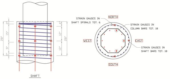
Figure 36. Diagrams. Strain gauge positions in the shaft.
The strains in the shaft reinforcing bars in both specimens are shown in figure 37 and figure 38. At 4 inches below the interface position, the strains recorded by the inner and outer gauges at the same position in the north bar in specimen DS-1 were similar. The strain gauge pair in the south bar in specimen DS-1 were damaged before testing. In the east bars, the two gauges gave nearly the same values until near the end of the test. The fact that the gauges gave nearly the same values implies that the bars were primarily in tension, with little bending.
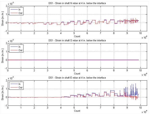
Figure 37. Graphs. Strain in shaft reinforcing bars in specimen DS-1.
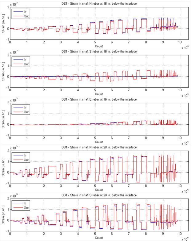
Figure 37. Graphs. Strain in shaft reinforcing bars in specimen DS-1, continued.
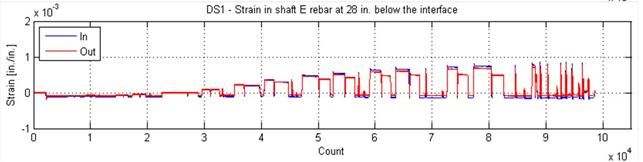
Figure 37. Graphs. Strain in shaft reinforcing bars in specimen DS-1, continued.
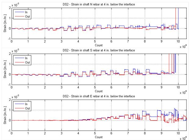
Figure 38. Graphs. Strain in shaft reinforcing bars in specimen DS-2.
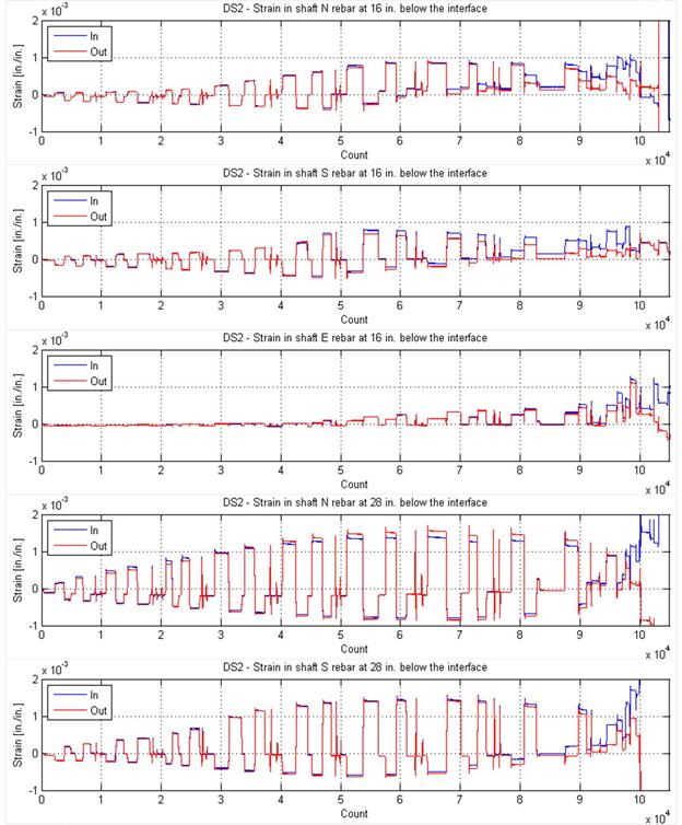
Figure 38. Graphs. Strain in shaft reinforcing bars in specimen DS-2, continued.
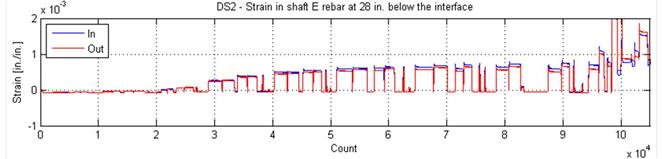
Figure 38. Graphs. Strain in shaft reinforcing bars in specimen DS-2, continued.
In specimen DS-2, the values of the strain gauge pairs in the north and south bars were relatively different from count = 40,000 (0.9 percent drift) to the end of the test. These differences in gauge readings suggest that local bending happened at these positions. As illustrated in the plots, local bending caused the outside strain gauges (red line) to experience less tension and the inside strain gauges (blue line) to experience more tension. This local bending occurred after the transition region of the shaft cracked and the spiral in it yielded. This behavior was not seen at the positions 16 and 28 inches below the interface in specimen DS-1, and it can only be seen at the very end cycles when the spirals of the shaft were broken in specimen DS-2.
The pattern of strains in the vertical bars of the shaft, 4 inches below the interface, is also consistent with the way that the shaft behaved. Before cycle 4-1 (0.7 percent drift, count = 29,000), the shaft was essentially uncracked, so it behaved like a beam made from continuous, uncracked material. Because the applied load consisted of both compression and bending, the vertical bar strains on the compression side were higher than the tension strains on the opposite side. However, when the shaft cracked (at cycle 4-1, 0.7 percent drift), the concrete could no longer resist tension. Then the tension strain at the top of the shaft was higher than the compression strain on the opposite side. This change in the strain pattern, from high compression to high tension, is the one seen in the gauge records.
The strain distributions (the average of each pair of gauge readings) over the height of the north, south, and east shaft bars at various drifts for specimen DS-1 and DS-2 are shown in figure 39. The strains were plotted up to 3.0 percent drift. Both specimens show similar strain profiles before 1.2 percent drift. Until 0.7 percent drift, tension strains at the top position (4 inches below the interface) were nearly zero in both specimens. The compression strains were higher, about 200. However, after 0.7 percent drift, the top of the shaft cracked vertically and diagonally, so the tension strain in the bars increased as explained above. After 1.2 percent drift, the strain profiles in specimens DS-1 and DS-2 were different. The tension strains increased when drift increased. However, the compression strains at 4 inches and 16 inches below the interface decreased. The compression strain decreased gradually in specimen DS-1 and suddenly in specimen DS-2. This suggested that the friction between the column surface and the shaft reduced gradually in specimen DS-1 and was lost suddenly and almost completely in specimen DS-2 because the compression strain values dropped to nearly zero. The increasing of compression strain at 28 inches below the interface indicated that, at this time, friction was still good at this position in both specimens.
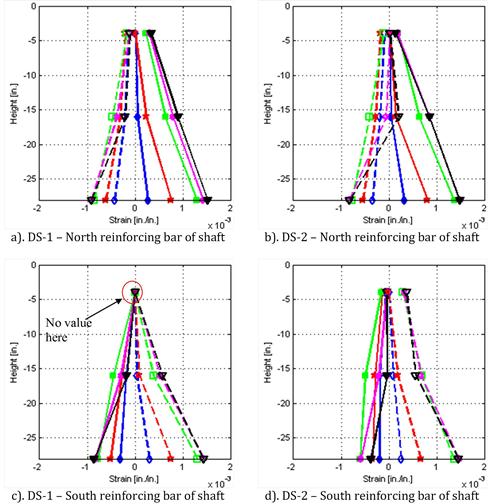
Figure 39. Graphs. Strain profiles in the shaft reinforcing bars.
Figure 40 shows the cyclic effective force-strain relationships of the shaft bars at 4, 16, and 28 inches below the interface, for specimens DS-1 and DS-2. In each plot, the cyclic effective force-strain relationship is plotted for the north, south, and east bars in blue, green, and purple, respectively. As illustrated, the strain values in all gauges in the shaft reinforcing bars were smaller than 0.002. This indicated that all the shaft-reinforcing bars remained elastic throughout the test.
At 4 inches below the interface, as shown in the figures, the strain gauges in the south bar in DS-1 were broken before testing. Up to 0.7 percent drift, the force-strain relationships in specimens DS-1 and DS-2 were similar. When the effective force reached 40 kips, the strains in the north, south, and east reinforcing bars were about 25, 0, and 200, respectively, in both specimens. This illustrates that, in both specimens, the south bars were subjected to more compression when the effective force increased and the north reinforcing bars were subjected to more compression when the effective force decreased. The relationships had a line of symmetry through effective force Feff = 0. At Feff = 0, all the bar strains were about -25. As was shown in the column bar behavior, this suggested that the friction between the column surface and the shaft was still good. When the cyclic drift went from 0.7 percent to 4.6 percent, the relationships in DS-1 and DS-2 were also similar. As illustrated in the graphs, the compression strain in the north bar in specimen DS-1 and the north and south bars in DS-2 decreased while the tension strain increased after each cycle. This suggested that, at this time, the shaft concrete was cracked in the top of the shaft, so the tensile force transferred to the reinforcing bars.
At 16 inches below the column-shaft interface position, the behaviors were nearly the same as at the previous position. Until 1.5 percent drift the relationships in both specimens were similar. The north and south reinforcing bars were still transferring more compression. The friction between the column surface and the shaft was still good in both specimen because the strain values at Feff = 0 were nearly -50. When drift went from 1.5 percent to 6.9 percent, DS-1 and DS-2 behaved differently. In DS-1, the strain values when Feff = 0 were increase a little bit, indicating the friction was decreased but still good. Therefore, the compression strains in the reinforcing bars were decreased gradually. The maximum effective forces remained about 60 kips. However, in DS-2, effective force decreased from about 50 kips to 35 kips. The strain values when Feff = 0 were not zero and increased after each cycle. It illustrated that, at this period, the concrete was cracked and could not sustain tensile forces. Therefore, most of the tension transferred to the spirals. Thus, when the strain in the spiral increased over the yielding point, it would have residual strain. Consequently, there would have been some force in the reinforcing bars and spirals when the horizontal load was released to zero.
At 28 inches below the interface position, the relationships were plotted up to 6.9 percent drift. As shown in the figures, the friction was still good, and the reinforcing bars were still in the elastic range in DS-1. In DS-2, before 4.6 percent drift, the behavior was similar to that in specimen DS-1. The friction was good, and the reinforcing bars remained elastic. However, after 4.6 percent drift, the friction was lost and the spirals were broken, and the strains in the rebar decreased dramatically.
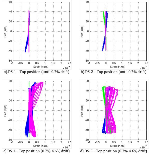
Figure 40. Graphs. Strain-Effective force relationship of the shaft reinforcing bars.
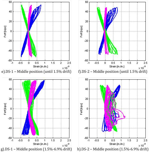
Figure 40. Graphs. Strain-Effective force relationship of the shaft reinforcing bars, continued.
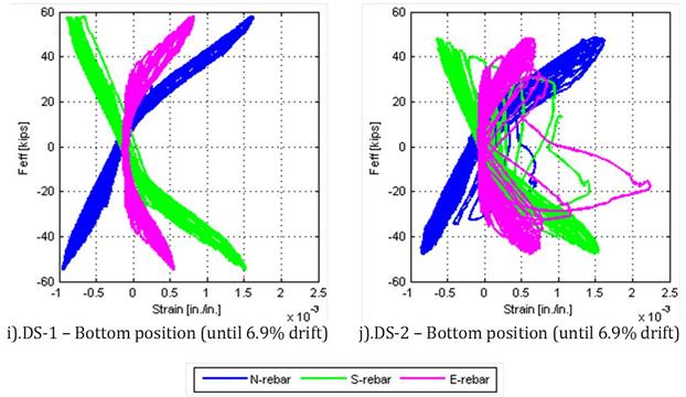
Figure 40. Graphs. Strain-Effective force relationship of the shaft reinforcing bars, continued.
Strains in Shaft Spirals
Because of the symmetry of the column longitudinal bars, only the east and south sides of the shaft spirals were gauged. In both specimens, gauges were attached on the spirals at three locations close to those of the gauges on the vertical bars - 4, 16, and 28 inches below the interface of the shaft and column. At each place, only one strain gauge was used.
The strains in the shaft spiral are shown in figure 41. Because all three gauges on the south side of specimen DS-1 were broken before testing, only the spiral strains on the east side in DS-1 and on the east and south sides in DS-2 were plotted.
The overall trends were as follows:
- In both specimens, the strains in the spiral were tensile regardless of the direction of loading.
- In both specimens, the strains were much larger at the top of the shaft than in the middle or bottom.
- The spiral in specimen DS-1 just reached the yield point. However, in specimen DS-2, the spiral first yielded at the top at 3 percent drift and fractured at 6.9 percent drift.
- The strain was slightly larger at the south gauge than at the east gauge, at any drift ratio, in specimen DS-2. That comparison was not possible in specimen DS-1 because no data were available from the south gauges.
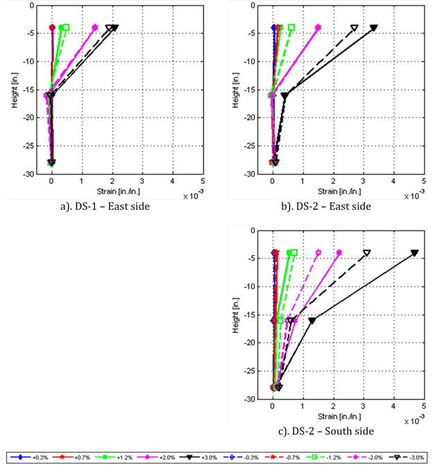
Figure 41. Graphs. Strain in shaft spiral.
The fact that the strains in specimen DS-2 were higher than those in specimen DS-1 is consistent with the lower spiral steel ratio in specimen DS-2.
As illustrated in the graphs, in specimen DS-1, tension strain increased at the top position after each cycle and reached 0.002 at 3.0 percent drift. At the middle position, strains were in compression and increased a little until 3.0 percent drift. At the bottom position, strains were nearly zero. However, the spiral strains in specimen DS-2 were different. All strain values were in tension at 3.0 percent drift. At the top position, the strains were in tension and increased after each cycle like in DS-1, but the values were higher. The maximum strain on the east side was about 3.4e-3, and on the south side it was 4.7e-3. At the middle position, until 2.0 percent drift, strain was nearly zero on the east side and increased to 0.4e-3 at 3.0 percent drift. On the south side, strains increased in tension after each cycle and reached 1.25e-3 at 3.0 percent drift. At the bottom position, the maximum strains were about 0.2e-3. This different behavior between specimens DS-1 and DS-2 suggests that, until 3.0 percent drift, friction between the column and shaft was lost from the interface position to some position above the mid-position (16 inches below the interface) in DS-1. However, in specimen DS-2, friction was lost at a position below the mid-position.