

Precast Bent System for High Seismic Regions: Laboratory Tests of Column-to-Drilled Shaft Socket Connections
DATA ANALYSIS
In bridges designed by WSDOT, the diameter of a drilled shaft is larger than that of the column that it supports. The splices between the longitudinal bars in the transition region are therefore non-contact splices, and special design requirements are necessary. McLean and Smith proposed a model for such a splice, and WSDOT has incorporated a modified version of it into the BDM.(11,18) However, the predictions of the modified model are not consistent with the test results from specimens DS-1 and DS-2. Therefore, a new conceptual model was developed to describe the observed behavior of the column-to-shaft "socket" connection.
First, the overall statically determinate test assembly was analyzed to give some guidance on parameters for design. Then, a simple strut-and-tie model was proposed to determine the amount of lateral reinforcement required in the connection. The proposed model is simple, easy to use in design, and consistent with the data from the two tests. However, because it is based on evidence from only two tests (DS-1 and DS-2), it cannot be guaranteed to provide correct predictions in all cases, and further testing is needed to support its use on a wider basis.
Non-Contact Lap Splices Models
McLean and Smith proposed both two-dimensional and three-dimensional models.(18) These models are based on the truss analogy to represent the force transfer mechanism within a splice.
Figure 42 illustrates a two-dimensional representation of the force transfer between non-contact longitudinal bars.
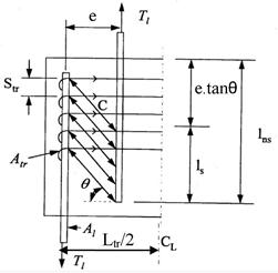
Figure 42. Diagram. Two-dimensional behavioral model for non-contact lap splices.
The transverse reinforcement is determined from the equation in figure 43.
Figure 43. Equation. Shaft transverse reinforcement for rectangular columns.
In this equation:
| Atr | = | area of shaft transverse reinforcement or spiral (in.2). |
| Al | = | total area of longitudinal column reinforcement (in.2). |
| fyt | = | specified minimum yield strength of shaft transverse reinforcement (ksi). |
| ful | = | specified minimum tensile strength of column longitudinal reinforcement (ksi), 90 ksi for A615 and 80 ksi for A706. |
| ls | = | Class C tension lap splice length of the column longitudinal reinforcement (in.). |
| str | = | spacing of shaft transverse reinforcement (in.). |
| θ | = | inclination angle of the strut (degree or rad). |
This equation indicates that a longer splice requires less spiral, and vice versa. For the special case of θ= 45° the equation becomes as shown in figure 44.
Figure 44. Equation. Shaft transverse reinforcement for rectangular columns with θ = 45°.
There is no unique definition for the optimum value of q to be used. One possible criterion is to use the q that minimizes the total volume of steel, including both longitudinal and transverse steel, required in the splice. It is given by the equation in figure 45.
Figure 45. Equation. Volume of shaft reinforcement for rectangular columns.
In figure 45:
| lns | = | total noncontact lap splice length. |
| = | lns = ls + e.tanθ | |
| Ltr | = | distance between the outer bars. |
Substituting figure 44 into figure 45 results in the equation in figure 46.
Figure 46. Equation. Volume of shaft reinforcement for rectangular columns - expanded equation.
The value of VOLs can be minimized by differentiating with respect to and setting the result to zero. This leads to the equation in figure 47.
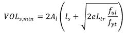
Figure 47. Equation. Minimum volume of shaft reinforcement for rectangular columns.
The inclination angle of the concrete strut can be determined using the equation in figure 48.
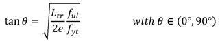
Figure 48. Equation. Inclination angle of the concrete strut.
The relationship of the total volume of steel used in the splice, VOLs, and the inclination angle of the strut, , are illustrated in figure 49 using the nominal properties of the splice in the test specimens:
- ful= 90 ksi
- fyt= 60 ksi
- Al= 10 x 0.31 = 3.1 in2
- ls= 22 in.
- e= 4 in.
- Ltr= 26 in.
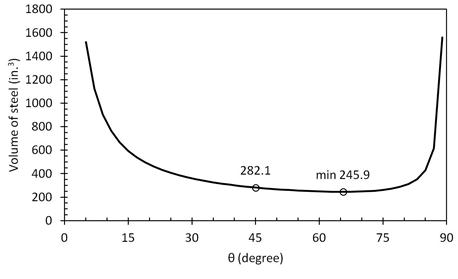
Figure 49. Graph. Relationship between the total steel volume in a splice and the inclined angle of struts.
At θ= 45°, the volume of steel in the splice is calculated as follows:
|
||
|
||
|
This analysis and the graph in figure 49 show that the minimum is very flat; even quite a large change in θ makes little difference to the total steel volume.
The foregoing model of a non-contact splice is two-dimensional and applies to rectangular tied columns. For a circular column, a three-dimensional model is needed. Such a model is illustrated in figure 50. It, too, is taken from MacLean and Smith, and it addresses loading in pure tension, rather than in bending.(18)

Figure 50. Diagrams. Proposed three-dimensional behavioral model for non-contact lap splices.(18)
The area of spiral reinforcement required in the transition region of the column-to-shaft connection, to fully develop the column reinforcing bars, is determined as shown in figure 51.
Figure 51. Equation. Shaft transverse reinforcement for circular columns.
The total volume of steel used in the splice, including both longitudinal and transverse steel, is determined as shown in figure 52.
Figure 52. Equation. Volume of shaft reinforcement for circular columns.
Substituting figure 51 into figure 52 results in the equation shown in figure 53.
Figure 53. Equation. Volume of shaft reinforcement for circular columns - expanded equation.
In figure 53:
| D | = | diameter of shaft spiral (in.). |
The minimum steel volume VOLs is given by the equation in figure 54.
Figure 54. Equation. Minimum volume of shaft reinforcement for circular columns.
The inclination angle of the concrete strut can be determined using the equation in figure 55.
Figure 55. Equation. Inclination angle of the concrete strut.
Using the nominal properties listed earlier, and D = 26 in., θ becomes θmin = 57.4°. At θ = 45° the volume of steel in the splice is calculated as follows:
The three-dimensional model was developed for a column in pure tension, in which all the bars are subjected to equal tension stress. In a column subjected to combined compression and bending, only some of the bars are in tension. Therefore, WSDOT modified the model before including in in the BDM, to the equation shown in figure 56.
Figure 56. Equation. Shaft transverse reinforcement for circular columns under axial load and bending.
In figure 56, k is a factor representing the ratio of column tensile reinforcement to total column reinforcement at the nominal resistance. The ratio is to be determined from column moment-curvature analysis or, as a default, taken as k = 0.5.
The length of the splices in specimens DS-1 and DS-2 was chosen as 28 inches. The spiral used in the splices was designed using the equation in figure 56 in specimen DS-1, and it was reduced by half in specimen DS-2. However, the measured strains from the gauges on the spirals of specimen DS-1 showed that the spirals at mid-height and the bottom of the transition region experienced almost no stress. Most of the transverse strain was concentrated in the top part of the transition region. In specimen DS-2 the spiral strain was much larger at the top and almost zero at the bottom. These data are inconsistent with the model predictions using the equation from McLean and Smith, because the model assumes that the spirals are fully stressed over the entire length of the splice.(18)
Column Moment-Curvature Analysis
To develop a method for column-shaft connection design, the distribution of longitudinal bar stresses round the column was needed. It was found using moment-curvature analysis. The validity of the analysis was confirmed by comparing the predicted and measured moments. Moment-curvature analysis was conducted using an in-house University of Washington program.(22) Two analyses were conducted, each with different material properties, and compared with test data from specimen DS-1.
The concrete model used in the program is based on the one proposed Kent and Park and is illustrated in figure 57.(15) Note that tension stress and tension strain are positive. It consists of a parabolic rising curve, followed by a linear falling segment, then a constant stress extending to infinite strain. In the program, the initial parabolic curve is replaced by a cubic, which allows the user to specify Ec0, c0 and f'c independently. It defaults to the original parabolic curve if Ec0 is chosen to be f'c/(2co). The strain at peak stress, = 0.002. However, here the values of the confined concrete strength, = 8 ksi, and the ultimate compression strain, =0.009, were generated from the properties of the confinement reinforcement using Mander's formula, rather than using the values recommended by Kent and Park.(16,17)
The steel model in the program contains three regions: elastic region, a yield plateau, and a curved strain-hardening region. In the first analysis, the expected steel reinforcement properties were used, in accordance with the AASHTO Seismic Guide Specifications.(13) These recommendations () are based on data collected by Caltrans.(23) The steel properties in the second analysis were based on the measured reinforcement properties for these tests (). The stress-strain curves for the reinforcing steel and concrete, and resulting moment-curvature relationships, are shown in figure 57 and 58. The flexural strengths from the two analyses and specimen DS-1 are shown in table 8.
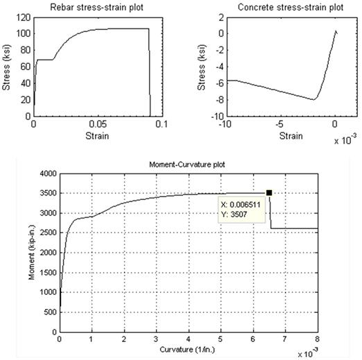
Figure 57. Graph. Moment-curvature analysis (based on expected material properties).
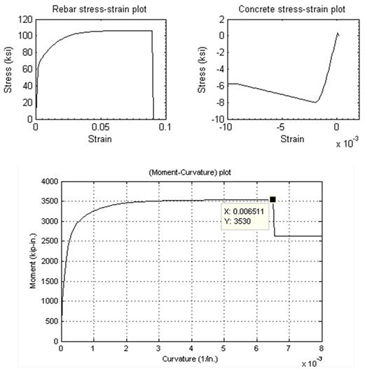
Figure 58. Graph. Moment-curvature analysis (based on measured material properties).
|
Analysis 1 (Expected Properties) (kip-in.) |
Analysis 2 (Measured Properties) (kip-in.) |
Measured (Specimen DS-1) (kip-in.) |
|---|---|---|
| 3507 | 3530 | 3476 |
The moments predicted by both analyses are close to the measured peak moment. These results suggest that the differences in longitudinal reinforcement properties do not affect the flexural strength of the column. Both analyses give the ultimate flexural strength at the curvature value of 0.0065. However, when curvature increases from about 0.0005 to 0.002, the moments in the two analyses are different. This occurs because, at those curvatures, the reinforcement strain in analysis 1 reaches the yield plateau region, whereas the reinforcement strain in analysis 2 starts going to the strain-hardening region. Thus, the tension force in reinforcement in analysis 2 is larger than in analysis 1, so the moment in analysis 2 is higher. Later, when the reinforcement strain reaches the fracture point, the difference in stress between in analysis 1 and analysis 2 is small. Therefore, the moments of column are equal in both analyses.
Figures 59 and 60 show a plot of moment vs. strain in the extreme tensile reinforcement, and they show the measured values for specimens DS-1 and DS-2 and the values predicted by the moment-curvature analyses. The curves were plotted up to the peak strain measured in the tests, of about 0.011. (At larger strains, the gauges continued to read but the data acquisition system saturated and simply displayed the saturation strain.) All curves include two regions: an elastic region and a curved post-yield region.
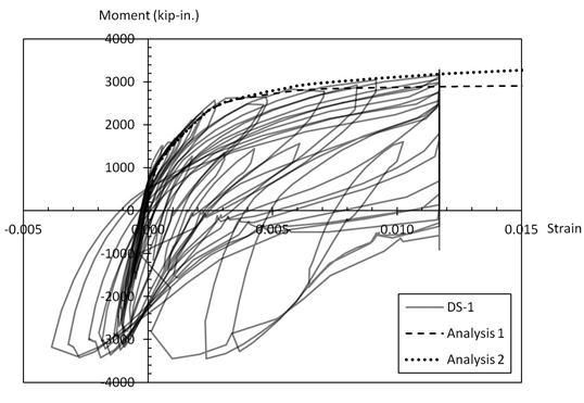
Figure 59. Graph. Moment-extreme reinforcement tensile strain relationship for column (in specimen DS-1).
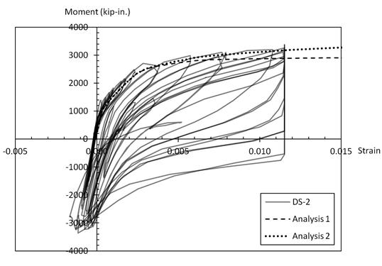
Figure 60. Graph. Moment-extreme reinforcement tensile strain relationship for column (in specimen DS-2).
The measured moments for a given strain in both specimens DS-1 and DS-2 are remarkably similar to the ones predicted in analysis 2, which used measured reinforcement properties. The moments in the post-yield region in analysis 1, using expected reinforcement properties, are smaller than the measured ones. At a strain of 0.0115, the measured moment is approximately 10 percent higher than the predicted one in analysis 1. This discrepancy, as mentioned earlier, is because of the yield plateau region of the expected steel model. In the confined concrete model, the strain at peak stress, is given as 0.002 instead of 0.0034 as in Mander's formula. If Mander's formula is used here, the predicted moments in the yield region in analysis 1 and 2 are approximately 10 percent and 20 percent smaller than the measured ones, respectively. It suggests that Mander's confined concrete model is inconsistent with the tests on specimens DS-1 and DS-2.
The shaft longitudinal reinforcement strain was smaller than 0.002 during the testing, so the shaft remained elastic. Figure 61 shows the relationship between moment at the base of the shaft and tensile strain in the extreme longitudinal reinforcement in the shaft at three different levels. The figure includes measured data from specimens DS-1 and DS-2 and moments predicted using measured material properties and strains at the bottom of the shaft. The analysis is comparable to analysis 2 for the column but used the shaft geometry. Note that the jump in the predicted curve at about 2,400 kip-in. indicates first cracking.
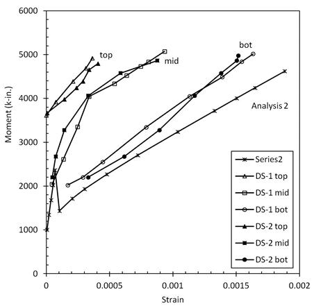
Figure 61. Graph. Relationship of moment at the base and extreme reinforcement tensile strain for the shaft.
Several features are evident.
For a given moment at the base of the shaft, the strains in the longitudinal shaft bars are the largest at the bottom and smallest at the top. This is as expected because it follows the trend of the moment diagram.
The measured strains from specimens DS-1 and DS-2 are remarkably similar. This similarity reflects the fact that, early in the load sequence, the load-deflection curves of the two specimens were similar.
The measured strains are smaller than the predicted ones. This is the opposite of what might be expected, for several reasons. First, application of a strain gauge involves some grinding and sanding of the bar, which inevitably reduces its area. For a given bar force, the measured strain is therefore likely to be higher than that obtained by dividing the nominal stress by E. Second, reinforcing bars tend to have areas that are, on average, less than the nominal value, but they have a higher true fy to compensate. However, because the Young's modulus is essentially unchanged, this tendency should be expected to lead to measured strains that are, again, higher than those predicted from the nominal material properties. Last, the bars are elastic, so increases in the yield strength cannot explain the difference.
The Strut-and-Tie Model and Shaft Spiral Design
The geometry of the transition region defines it as a "disturbed region" in which Engineering Beam Theory is not applicable. Other methods, such as the strut-and-tie method, must be used to model the behavior of the column-shaft connection. Schlaich and Schäfer proposed two models for a socket footing.(24) One has smooth surfaces, and the other has rough surfaces between the column and the walls of the socket (see figure 62).
For the geometry used in specimens DS-1 and DS-2, the model for the column-shaft connection with a smooth surface leads to a horizontal force T2 of approximately150 kips when V = 50 kips, and an additional tensile force T4 of approximately 100 kips at the bottom of the transition. To resist these forces, 55 turns of spiral of the size used in the tests would be needed at the top and 36 turns at the bottom of the transition, whereas specimen DS-1 had a total of 24 turns and specimen DS-2 had 12. Thus, when the specimens reached their peak loads, the distribution of internal forces cannot have been the same as in the smooth surface model. However, at the very end of the specimen DS-2 test, when contact between the column surface and shaft surface was lost and friction was no longer possible, the specimen is believed to have behaved like the smooth surface model. At that stage, the loads were much smaller, and the low capacity of the spiral was consistent with the low load.
In the tests on specimen DS-1, no vertical slip at the interface was observed. The tie forces in the test were much smaller than those needed for the smooth model. Thus, the rough surface model for the column-shaft connection appears to be more consistent with the observed behavior. However, Schlaich and Schäfer's model is for a two-dimensional system, so it was necessary to perform a three-dimensional analysis for the circular column used in the tests. Figure 63 illustrates the model.
The column contained 10 No. 5 bars and the shaft contained 30 pairs of No. 3 bars. Thus, the tension force, T, in any column bar is assumed to transfer to the three nearest bar pairs of shaft reinforcement, as indicated in figure 64. The angle of inclination between struts C1 and C3 and the horizontal is taken to be . To simplify the analysis, the longitudinal reinforcement in the column and shaft was assumed to be distributed continuously round the perimeter, rather than as discrete bars, and the strut C1 directions are radial, as shown in figure 65. The horizontal component of the strut force C1 is T1/tan, and this is therefore the radial force per unit length applied to the shaft spiral. The distribution of tension T1 in the shaft longitudinal bars is calculated by using the proposed moment-curvature analysis.
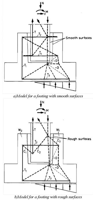
Figure 62. Diagram. Strut-and-tie model proposed by Schlaich and Schäfer.(24)
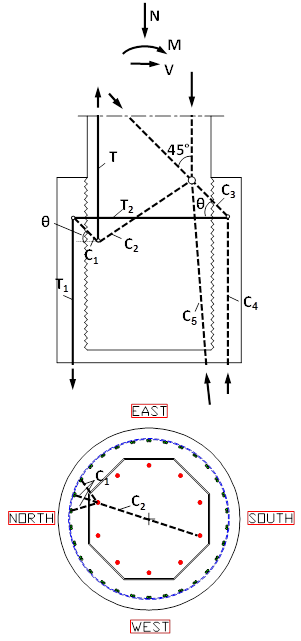
Figure 63. Diagrams. Elevation and plan of the strut-and-tie model for transmitting load from one column reinforcing bar to the three nearest shaft bundles bars.
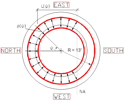
Figure 64. Diagram. Tension transfer from column to shaft longitudinal reinforcement.
As indicated in figure 64, the distributed load, p applied around the circumference of the shaft spiral is given by the equation in figure 65.
Figure 65. Equation. Distributed load determination.
The distribution of tension in the shaft reinforcement is obtained using the equation in figure 66.
Figure 66. Equation. Distribution of tension in the shaft reinforcement.
In figure 66:
| Al,sh | = | total area of longitudinal shaft reinforcement (in.2). |
| fs | = | tensile stress in shaft reinforcement (ksi). |
| εs | = | tensile strain in shaft reinforcement. |
| L(ψ) | = | distance from the neutral axis to the tension longitudinal reinforcement. |
| Es | = | modulus of elasticity of reinforcement (ksi). |
| R | = | radius of shaft spiral (in.). |
| Φ | = | curvature (1/in.). |
| ψ | = | angular coordinate (rad). |
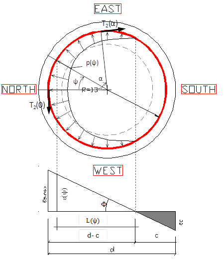
Figure 67. Diagram. Distributed load applied to shaft spirals.
From the strain distribution in figure 67, we have:
Figure 68. Equation. Distance of tensile forces from the neutral axis.
In figure 68:
| d | = | distance from the extreme compression fiber to the extreme tension longitudinal reinforcement. |
| c | = | depth to the neutral axis. |
Substituting L(ψ) in the equation in figure 67 results in the equation shown in figure 69.
Figure 69. Equation. Distribution of tension in the shaft longitudinal reinforcement.
Substituting T1(ψ) in the equation in figure 65 results in the equation shown in figure 70.
Figure 70. Equation. Distributed load applied to the shaft transverse reinforcement.
Summing the north-south horizontal forces leads to the equation shown in figure 71.
In figure 71, α is an angular coordinate measured from the north.
Substituting figure 70 in figure 71 yields the equation shown in figure 72.
The parameters used in the tests were as follows:
- R = 13 in.
- Al = 30*0.22 = 6.6 in.2
- Es = 29000 ksi
- d = 28 in.
- c = 9 in.
If θ is assumed to be 45 degrees, and the curvature is taken when the predicted moment is equal to the peak measured moment (Φ = 106.11 e-6 in.-1), the distribution of the tensile force, T2, in the shaft spirals is shown in figure 73.
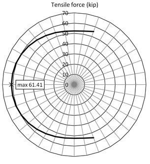
The maximum tensile force in the tie, T2, occurs at α = 0.0, and is calculated using the equation in figure 74.
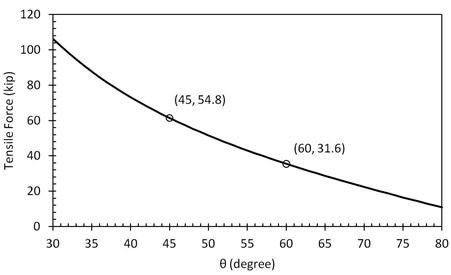
The relationship between the maximum spiral force, T2,max, and the assumed strut inclination angle, θ, is shown in figure 75. As might be expected, steeper strut angles lead to lower spiral forces.
The strut angle can be estimated by equating the spiral capacity and demand. The yield strength of a single spiral wire is calculated as shown in figure 76.
If all 24 turns of the spiral in specimen DS-1 were to be active in the load transfer, the total spiral capacity would be 24*1.376 = 33.0 kips, for which figure 75 shows a corresponding strut angle of 62 degrees. However, the measured strains in specimen DS-1 showed that only the spiral in the top of the transition region was stressed significantly. If only the spiral at the 15-inch upper transition (i.e., 16 turns) was active, the force would have been 22.0 kips and the angle close to 70 degrees. The assumed 16 active spirals is probably too high, given the strain distribution in the spiral. However if less spiral is assumed to be active, the strut angle becomes steeper. This 70-degree angle is sufficiently steep that it is improbable, both because the space for such a strut is not available and because it implies a low ratio of radial force to shear force being transferred across the column-to-shaft interface. The latter implies a friction coefficient significantly greater than 1.0.
In fact, the concrete may have provided some of the hoop tension force. If the concrete surrounding each spiral is taken into account, and the concrete width is taken as the thickness of the concrete annulus outside column, 5 inches, the strength of the surrounding concrete per unit length is calculated as follows:
where:
| f r | = | concrete modulus of rupture. |
| = |
If the strut angle is taken as θ = 45 degrees, which implies a friction coefficient equal to 1.0, figure 75 shows a maximum tensile force of 54.8 kips. At the upper transition, the strength of the spirals is 22 kips, as mentioned above. Thus, the necessary length of concrete is calculated as follows:
The necessary length of concrete is smaller than the assumed length of upper transition (15 inches), so this assumption seems to be plausible. If the designers do not want to rely on the concrete tensile strength, they can increase the number of spirals 2.5 times to get a strength of 55 kips.
This suggests that the spiral was at yield stress (80 ksi, ε = 0.003) at the upper transition while the concrete was still uncracked (fr = 630 psi, ε = 0.630 / 5000 = 0.00012) at the lower transition.