

Executive Summary
Chapter 1
Household Travel in America
Over 300 million people in the United States make decisions about travel every day with about three-quarters of the vehicle miles traveled (VMT) on the Nation’s roadways for purposes of personal travel. The household travel data cited below are drawn primarily from a sampling of Americans’ daily travel habits collected in the National Household Travel Survey (NHTS).
How People Use the Transportation System
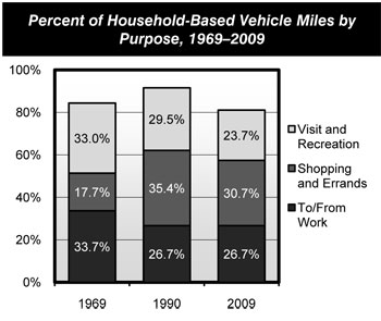
Travel to and from work accounted for 26.7 percent of household-based vehicle travel in 2009, compared with 33.7 percent in 1969; the share of trips devoted to personal visits and recreation also declined. The share of trips attributed to shopping and errands grew significantly over this period from 17.7 percent to 30.7 percent. These trips had widely different destinations than work trips and occurred at different times of day.
Recent data on work commute trends show an increase in telecommuting and flexible hours in the U.S. workplace. More than 36 percent of full-time workers can set or change their start time. The data show that workers are increasingly linking commuting with trips for non-work activities such as errands and shopping. These non-work trips have the potential to conflict with work commute trips and extend the a.m., p.m., and midday peak travel periods as well. Weekend travel for errands and recreation is also increasing.
While congestion used to be associated only with peak travel hours, the increasing share of trips unrelated to work presents a challenge for the operational performance of the transportation system at other times as well.
Travel to work has historically defined peak hour travel demand and in turn influenced the design of transportation infrastructure. Work trips are a critical factor to transit planning and help to determine corridors served and assess the level of transit services available. The average automobile commuter spends 22.8 minutes commuting a one-way distance of 12.6 miles; bus commuters travel a shorter average distance of 9.4 miles, but have a higher average commuting time of 48.9 minutes.
| Travel Mode | Time, minutes | Distance, miles | Estimated Speed, mph |
|---|---|---|---|
| Walk | 14.2 | 1.1 | 4.8 |
| Privately Owned Vehicle | 22.8 | 12.6 | 33.2 |
| Bus | 48.9 | 9.4 | 11.5 |
| Commuter Rail | 51.7 | 12.2 | 14.1 |
Shifting Travel Patterns
Socio-demographic changes in the United States are expected to impact travel patterns in coming years. First, while older drivers tend to reduce their daily travel relative to when they were younger, these older drivers are expected to constitute a significantly higher share of total national travel in the future as the baby boom generation ages. Second, 18 million of 150 million U.S. households are made up of new immigrants who tend to have a larger number of persons per household, a greater number of daily household trips, and less likelihood of owning a vehicle; increased immigration can have implications such as increased carpooling, walking, biking, and use of public transit. Third, population redistribution within the United States, such as shifts from the Northeast and Midwest to the Southern and Western States, has the potential to overwhelm the transportation systems in some of these redistributed areas.
Chapter 2
System Characteristics: Highways and Bridges
In 2008, a network of 4.1 million miles of public roads provided mobility for the American people. Rural areas accounted for 73.4 percent of this mileage. While urban mileage constitutes only 26.6 percent of total mileage, these roads carried 60.1 percent of the almost 3.0 trillion vehicle miles traveled (VMT) in the United States in 2008. Urban areas are defined to include all places with a population of 5,000 or greater; all other locations are classified as rural.
In 2009, 25.9 percent of the Nation’s 603,310 bridges were located in urban areas; these bridges carried 76.3 percent of total bridge traffic and included 55.9 percent of the total bridge deck area.
Roadways functionally classified as rural local made up 50.2 percent of total mileage in 2008, but carried only 4.4 percent of total VMT. In contrast, the urban portion of the Interstate System made up only 0.4 percent of total mileage but carried 15.2 percent of total VMT.
| Functional System | 2008 Miles | 2008 VMT | 2009 Bridges |
|---|---|---|---|
| Rural Areas | |||
| Interstate | 0.7% | 8.1% | 4.2% |
| Other Principal Arterial | 2.3% | 7.4% | 5.9% |
| Minor Arterial | 3.3% | 5.1% | 6.4% |
| Major Collector | 10.3% | 6.2% | 15.4% |
| Minor Collector | 6.5% | 1.8% | 8.0% |
| Local | 50.2% | 4.4% | 34.2% |
| Subtotal Rural | 73.4% | 33.1% | 74.1% |
| Urban Areas | |||
| Interstate | 0.4% | 16.1% | 4.9% |
| Other Freeway and Expressway | 0.3% | 7.5% | 3.2% |
| Other Principal Arterial | 1.6% | 15.6% | 4.5% |
| Minor Arterial | 2.6% | 12.7% | 4.6% |
| Collector | 2.8% | 5.9% | 3.3% |
| Local | 18.8% | 9.1% | 5.3% |
| Subtotal Urban | 26.6% | 66.9% | 25.9% |
| Total | 100.0% | 100.0% | 100.0% |
Highway mileage increased at an average annual rate of 0.3 percent between 2000 and 2008, while VMT grew at an average annual rate of 1.0 percent.
In 2008, 77.4 percent of highway miles were locally owned, 19.3 percent were owned by States, and 3.2 percent were owned by the Federal government. Bridge ownership is more evenly split; in 2009, 50.2 percent of bridges were locally owned, while 48.1 percent were owned by States.
The term “Federal-aid highways” applies to the subset of the road network that is generally eligible for Federal funding assistance under most programs; this includes all functional systems except for rural minor collector, rural local, and urban local. (Certain programs have broader eligibility criteria that allow funds to be used for any type of road). Federal-aid highways represent 24.5 percent of total mileage and carry 84.7 percent of total VMT.
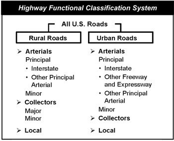
The 162,944-mile National Highway System (NHS) includes the Nation’s key corridors and carries much of its traffic. In 2008, NHS included only 4.0 percent of the Nation’s total route mileage and only 6.7 percent of the Nation’s total lane miles, but 44.3 percent of VMT in the Nation were on the NHS. Of the total bridges in the Nation, only 19.5 percent are on the NHS; but these bridges comprise 49.2 percent of the total bridge deck area of the Nation.
All of the Interstate System is part of the NHS, as are 83.5 percent of rural other principal arterials, 87.1 percent of urban other freeways and expressways, and 36.3 percent of urban other principal arterials.
Chapter 2
System Characteristics: Transit
Transit system coverage, capacity, and use in the United States continued to increase between 2006 and 2008. In 2008, there were 690 agencies (667 public agencies) in urbanized areas required to submit data to the National Transit Database (NTD). All but 166 of these agencies operated more than one mode. There were also 1,396 rural transit operators that reported. Urban reporters operated 658 motor bus systems, 633 demand response systems, 16 heavy rail systems, 29 commuter rail systems, and 35 light rail systems. There were also 67 transit vanpool systems, 20 ferryboat systems, 7 trolleybus systems, 4 automated guideway systems, 4 inclined plane systems, and 1 cable car system. Not all transit providers are included in these counts since those that do not receive grant funds from the Federal Transit Administration (FTA) are not required to report to the NTD.
These systems operated 73,512 motor buses, 29,833 vans, 11,367 heavy rail vehicles, 6,124 commuter rail cars, and 1,919 light rail cars. Transit providers operated 11,864 miles of track and served 3,078 stations. Light rail systems have been growing fastest since 2006, with track mileage up 5.1 percent and the number of stations served up 3.0 percent. Nonetheless, the Nation’s rail system mileage is still dominated (62 percent) by commuter rail. Trends in directional route miles follow growth in track mileage and allow for comparison with nonrail modes.
| Transit Mode | 2000 | 2008 | Change 2000–2008 |
|---|---|---|---|
| Rail | 9,222 | 11,270 | 22.2% |
| Commuter Rail | 6,802 | 8,219 | 20.8% |
| Heavy Rail | 1,558 | 1,623 | 4.2% |
| Light Rail | 834 | 1,397 | 67.5% |
| Other Rail | 29 | 30 | 5.2% |
| Nonrail | 196,858 | 212,801 | 8.1% |
| Bus | 195,884 | 211,664 | 8.1% |
| Ferryboat | 505 | 682 | 34.9% |
| Trolleybus | 469 | 456 | -2.8% |
| Total | 206,080 | 224,071 | 8.7% |
| Percent Nonrail | 95.5% | 95.0% |
In 2008, transit services provided 10.2 billion unlinked trips and 53.7 billion passenger miles traveled (PMT). Heavy rail and motor bus modes continue to be the largest segments of both measures. Commuter rail supports relatively more PMT due to its greater average trip length (23.4 miles compared with 3.9 for bus, 4.8 for heavy rail, and 4.4 for light rail). Light rail is the fastest-growing rail mode (with PMT growing at 5.7 percent per year between 2000 and 2008) but still provides only 3.9 percent of transit PMT in 2008. Vanpool growth during that period was 11.8 percent per year, substantially outpacing the 1.8 percent growth in motor bus passenger miles, but while motor buses provided 39.5 percent of all PMT, vanpools accounted for only 1.8 percent.
| Transit Mode | 2000 | 2008 | Change 2000–2008 |
|---|---|---|---|
| Rail | 24,604 | 29,989 | 21.9% |
| Heavy Rail | 13,844 | 16,850 | 21.7% |
| Commuter Rail | 9,400 | 11,032 | 17.4% |
| Light Rail | 1,340 | 2,081 | 55.3% |
| Other Rail | 20 | 26 | 30.0% |
| Nonrail | 20,497 | 23,723 | 15.7% |
| Motor Bus | 18,807 | 21,198 | 12.7% |
| Demand Response | 588 | 844 | 43.5% |
| Vanpool | 407 | 992 | 143.7% |
| Ferryboat | 298 | 390 | 31.0% |
| Trolleybus | 192 | 161 | -16.3% |
| Other Nonrail | 205 | 138 | -32.7% |
| Total | 45,101 | 53,712 | 19.1% |
| Percent Rail | 54.6% | 55.8% |
Rural transit operators reported 136.6 million unlinked passenger trips on 486 million vehicle revenue miles. This included 61 Indian tribes who provided 417,000 unlinked passenger trips. Rural systems provide both traditional fixed-route and demand response services, with 1,150 demand response systems, 494 motor bus systems, and 16 vanpool systems. A total of 304 urbanized area agencies also reported providing rural service at the rate of 24 million unlinked passenger trips on 37 million vehicle revenue miles in 2008. Every state reported providing rural service.
Chapter 3
System Conditions: Highways and Bridges
Poor pavement condition imposes economic costs on highway users in the form of increased wear and tear on vehicle suspensions and tires, delays associated with vehicles slowing to avoid potholes, and crashes resulting from unexpected changes in surface conditions. While transportation agencies consider many factors when assessing the overall condition of highways and bridges, surface roughness most directly affects the ride quality experienced by drivers.
On the NHS, the percentage of VMT on pavements with good ride quality has risen sharply over time, from approximately 48 percent in 2000 to about 57 percent in 2008. (These calendar year values are identified as fiscal year 2001 and 2009 values in some other U.S. DOT publications.) The VMT on NHS pavements meeting the acceptable standard of ride quality increased from 91 percent in 2000 to 92 percent in 2008.
| Ride Quality | Calendar Year 2000 | Calendar Year 2004 | Calendar Year 2008 |
|---|---|---|---|
| Good (IRI < 95) | 48% | 52% | 57% |
| Acceptable (IRI ≤ 170) | 91% | 91% | 92% |
Rural NHS routes tend to have better pavement conditions than urban NHS routes. In 2008, for example, about 97.5 percent of all VMT on rural pavements was traveled on routes with acceptable ride quality. By contrast, the portion of urban NHS VMT on acceptable pavements was 89.0 percent that same year.
For Federal-aid highways as a whole, including the NHS and other arterials and collectors eligible for Federal funding, the VMT on pavements with good ride quality increased from 42.8 percent in 2000 to 46.4 percent in 2008. The VMT on pavements meeting the less stringent standard of acceptable ride quality declined slightly from 85.5 percent in 2000 to 85.4 percent in 2008.
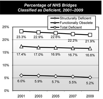
Two terms used to summarize bridge deficiencies are “structurally deficient” and “functionally obsolete.” Structural deficiencies are characterized by deteriorated conditions of significant bridge elements and potentially reduced load-carrying capacity. A “structurally deficient” designation does not imply that a bridge is unsafe, but such bridges typically require significant maintenance and repair to remain in service, and would eventually require major rehabilitation or replacement to address the underlying deficiency. A bridge is considered “functionally obsolete” when it does not meet current design standards (for criteria such as lane width), either because the volume of traffic carried by the bridge exceeds the level anticipated when the bridge was constructed and/or the relevant design standards have been revised. Addressing functional deficiencies may require the widening or replacement of the structure. Rural bridges tend to have a higher percentage of structural deficiencies, while urban bridges have a higher incidence of functional obsolescence due to rising traffic volumes.
The share of total bridges classified as deficient (meaning the share of bridges classified as either structurally deficient or functionally obsolete) fell from 30.1 percent in 2001 to 26.5 percent in 2009. The share of NHS bridges classified as deficient fell from 23.3 percent in 2001 to 21.9 percent in 2009; this reduction was split evenly between structurally deficient and functionally obsolete bridges.
Chapter 3
System Conditions: Transit
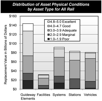
This edition of the C&P report discusses levels of investment needed to achieve a “state of good repair” benchmark. The Federal Transit Administration (FTA) uses a numerical condition rating scale ranging from 1 to 5 (detailed in Chapter 3) to describe the relative condition of transit assets as estimated by the Transit Economic Requirements Model (TERM). Assets are considered to be in a state of good repair when the physical condition of that asset is at or above a condition rating value of 2.5 (the mid-point of the marginal range). An entire transit system is in a state of good repair when all its assets are rated at or above the 2.5 threshold rating. This report estimates the cost of replacing all assets in the national inventory that are past their useful life (that is, below the 2.5 condition rating) to be a total of $78 billion. This is 12 percent of the estimated total asset value of $663.3 billion for the entire U.S. transit industry.
| Asset Type | Replacement Value Nonrail |
Replacement Value Rail |
Replacement Value Joint Assets |
Total |
|---|---|---|---|---|
| Maintenance Facilities | $56.4 | $33.2 | $3.8 | $93.4 |
| Guideway Elements | $13.1 | $234.5 | $1.0 | $248.6 |
| Stations | $3.8 | $84.8 | $0.6 | $89.1 |
| Systems | $3.4 | $107.5 | $1.3 | $112.2 |
| Vehicles | $41.1 | $78.5 | $0.5 | $120.1 |
| Total | $117.7 | $538.6 | $7.0 | $663.3 |
The cost-weighted average condition rating over all bus types is near the bottom of the adequate range (3.18) where it has been without appreciable change for the past decade. Average age is up slightly in all categories (except vans) as is the percentage of vehicles that is below the state of good repair replacement threshold. This is in spite of the fact that new vehicles have entered the fleet faster than at any time in the past decade. The number of vehicles reported is up 17 percent over the last 2 years. This is particularly evident with articulated buses (extra-long buses with two connected passenger compartments), which have grown in number by 25 percent. The average age of the bus fleet is now 6.2 years.
The cost-weighted average condition rating over all rail vehicles is near the middle of the adequate range (3.47) where it has been without appreciable change for the past decade. With average conditions and ages being quite stable over the last 5 years, the most significant aspect of the rail vehicle data presented here is the recent growth in the size of the fleet, which increased by 16 percent, both in total and for each of the individual modes, between 2006 and 2008. This is the largest increase observed over the past decade by far.
Non-vehicle transit rail assets represent the biggest challenge to achieving a state of good repair. The replacement value of guideway elements (track, ties, switches, ballast, tunnels, and elevated structures) is $143.6 billion, of which $19.1 billion is in poor condition (13 percent) and $15.8 billion is in marginal condition. The replacement value of train systems (power, communication, and train control equipment) is $92.0 billion, of which $13.7 billion is in poor condition (15 percent) and $18.9 billion is in marginal condition. The relatively large proportion of guideway and systems assets that are in poor condition, and the magnitude of the $38.2 billion investment required to replace them, represents a major challenge to the rail transit industry.
Chapter 4
Operational Performance: Highways
Drivers continue to experience high levels of congestion on the Nation’s highways, leading to travel delays, wasted fuel, and billions of dollars in congestion costs. From an economic perspective, travel time accounts for almost half of all costs experienced by highway users (other key components of user costs include vehicle operating costs and costs associated with crashes).
Three key aspects of congestion are severity, extent, and duration. Severity refers to the magnitude of the problem at its worst. The extent of congestion is the geographic area or number of people affected. Duration of congestion is the length of time that the traffic is congested, often referred to as the “peak period.” Since there is no universally accepted definition of exactly what constitutes a congestion “problem,” this report uses several metrics to explore different aspects of congestion.
The Texas Transportation Institute (TTI) collects data for 458 urban communities of different sizes across the Nation. The TTI 2009 Urban Mobility Report estimates that drivers experienced nearly 4.2 billion hours of delay and wasted approximately 2.8 billion gallons of fuel in 2007. The total congestion cost for these areas (including the implicit value that travelers place on their lost time) was $87.2 billion.
The Travel Time Index measures the amount of additional time required to make a trip during the congested peak travel period. The average value for all urbanized areas was 1.24 in 2008, indicating that a trip during the peak period would require 24 percent longer than the same trip during off-peak noncongested conditions. For example, a trip of 60 minutes during the off-peak time would require 74.4 minutes during the peak period.
The average Travel Time Index for all urbanized areas had begun to decline in recent years, dropping below its 2000 level of 1.25. This reduction occurred primarily in areas with a population of 1 million or greater. Smaller urbanized areas did not experience the same degree of reduced congestion based on the Travel Time Index or other measures.
| Urbanized Area Population | Year 2000 | Year 2004 | Year 2008 |
|---|---|---|---|
| Less Than 500,000 | 1.11 | 1.12 | 1.11 |
| 500,000 to 999,999 | 1.16 | 1.18 | 1.16 |
| 1 Million to 3 Million | 1.24 | 1.26 | 1.23 |
| Over 3 Million | 1.36 | 1.39 | 1.35 |
| All Urbanized Areas | 1.25 | 1.27 | 1.24 |
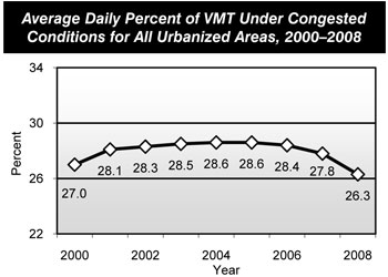
The average daily percentage of VMT under congested conditions is a metric that indicates the portion of daily traffic on freeways and other principal arterials in an urbanized area that moves at less than free-flow speeds. After increasing from 27.0 percent to 28.6 percent in 2004, this percentage dropped to 26.3 percent in 2008. This decrease can partially be attributed to the reduction in VMT that occurred between 2006 and 2008.
There are different ways in which congestion can be measured. The CEOs for Cities “Driven Apart” report suggests an alternative approach to the TTI methodology. This report is available at: http://www.ceosforcities.org/driven-apart.
A variety of strategies can contribute to reducing congestion. These include the strategic addition of new capacity, increasing the productivity of existing capacity via systems management and operations, providing transportation alternatives along congested corridors, and travel demand management through approaches such as congestion pricing.
Chapter 4
Operational Performance: Transit
Transit operational performance can be measured and evaluated using a number of different factors, including the speed of passenger travel, vehicle utilization, and service frequency.
Average operating speed in 2008 remained consistent with 2006 levels at 19.5 miles per hour across all transit modes. Average operating speed is an approximate measure of the speed experienced by transit riders and is affected by dwell times and the number of stops. The average speed of nonrail modes was 13.7 miles per hour in 2008, the same as was reported in 2000. Rail mode operating speeds have decreased from 24.9 miles per hour in 2000 to 23.9 miles per hour in 2008.
Average vehicle occupancy levels did not change significantly between 2000 and 2008. The most significant changes over that period were a 7.5 percent increase for heavy rail and a 7.6 percent decrease for light rail. Light rail decreases may be due to the addition of new capacity in that mode over this period. Several urbanized areas, including Denver, Phoenix, Seattle, Charlotte, and Salt Lake City, opened new light systems during this period of time. The nonrail modes were practically unchanged.
Adjusting for the number of seats on an average vehicle for each mode, it can be seen that, as expected, vanpool and heavy rail vehicles, on the average, run closer to capacity than other modes.
| Transit Mode | Passenger Count | Seat Count | Percent Occupied |
|---|---|---|---|
| Demand Response | 1.2 | 10 | 12.3% |
| Motor Bus | 10.8 | 39 | 27.8% |
| Commuter Rail | 35.7 | 126 | 28.3% |
| Ferryboat | 118.1 | 405 | 29.2% |
| Trolleybus | 14.3 | 47 | 30.4% |
| Light Rail | 24.1 | 63 | 38.3% |
| Heavy Rail | 25.7 | 53 | 48.5% |
| Vanpool | 6.3 | 11 | 57.5% |
Between 2000 and 2008, transit agencies have provided substantially more vanpool, demand response, and light rail service. These modes have far outpaced motor bus, with its 1.3 percent per year growth rate in revenue miles, and heavy rail with its 1.6 percent growth rate. Vanpool, growing at almost 12.3 percent per year, is set to become a major mode. Demand response is starting to account for a great number of service miles, though with an average of only 1.2 passengers, it is still a small contributor to the total number of passenger trips.
| Transit Mode | 2000 | 2008 | Change 2000–2008 |
|---|---|---|---|
| Rail | 879 | 1,053 | 19.8% |
| Heavy Rail | 578 | 655 | 13.3% |
| Commuter Rail | 248 | 309 | 24.6% |
| Light Rail | 51 | 86 | 68.6% |
| Other Rail | 2 | 3 | 50.0% |
| Nonrail | 2,322 | 2,840 | 22.3% |
| Motor Bus | 1,764 | 1,956 | 10.9% |
| Demand Response | 452 | 688 | 52.2% |
| Vanpool | 62 | 157 | 153.2% |
| Ferryboat | 2 | 3 | 50.0% |
| Trolleybus | 14 | 11 | -21.4% |
| Other Nonrail | 28 | 25 | -10.7% |
| Total | 3,201 | 3,893 | 21.6% |
Productivity per active vehicle increased between 2000 and 2008. Vehicle in-service mileage has increased steadily from 2000 to 2008 for all the major modes. Light rail has shown particularly strong growth, though from a low starting point. Demand response has also shown a strong improvement in vehicle miles per active vehicle.
| Mode | Thousands of Vehicle Revenue Miles 2000 |
Thousands of Vehicle Revenue Miles 2008 |
Average Annual Rate of Change2008/2000 |
|---|---|---|---|
| Rail | 130.2 | 147.3 | 1.6% |
| Heavy Rail | 55.6 | 57.7 | 0.5% |
| Commuter Rail | 42.1 | 45.5 | 1.0% |
| Light Rail | 32.5 | 44.1 | 3.9% |
| Nonrail | 101.9 | 106.5 | 0.6% |
| Motor Bus | 28.0 | 30.3 | 1.0% |
| Demand Response | 17.9 | 21.3 | 2.2% |
| Ferryboat | 24.1 | 21.9 | -1.2% |
| Vanpool | 12.9 | 14.3 | 1.3% |
| Trolleybus | 18.9 | 18.7 | -0.1% |
Chapter 5
Safety: Highways
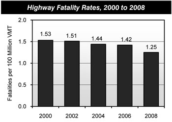
There has been considerable progress in reducing the number of highway fatalities since 1966, when Federal legislation first addressed highway safety. That year, the fatality rate was 5.50 fatalities per 100 million vehicle miles traveled (VMT). This figure dropped to 1.53 in 2000 and 1.25 in 2008. The total number of highway fatalities decreased from 41,945 in 2000 to 37,261 in 2008. (Preliminary data for 2009 indicate further declines in the fatality rate to 1.13; highway fatalities dropped to 33,808 in 2009, the lowest number since 1950.)
From 2000 to 2008, the number of fatalities on urban roadways decreased by about 1 percent from 16,113 to 15,983. During this same period, fatalities on rural roads decreased by almost 16 percent from 24,838 to 20,905. Urban Interstate highways were the safest functional system, with a fatality rate of 0.47 per 100 million VMT in 2008. Although the fatality rate on rural local roads declined from 3.45 to 3.08 per 100 million VMT from 2000 to 2008, this functional system continues to have the highest fatality rate.
Approximately 53 percent of highway fatalities in 2008 involved a roadway departure, in which a vehicle left its travel lane and crashed. While roadway design and environmental factors play a role in these types of crashes, behavioral factors such as driver intoxication, driver fatigue, driver drowsiness, and driver distraction also have a significant impact. Some roadway departures can be attributed to drivers being distracted while attempting to operate mobile devices. The U.S. DOT is leading efforts to help educate drivers and promote a greater understanding of the issue.
In 2008, approximately 21 percent of highway fatalities occurred at intersections. Of these fatalities, about 61 percent occurred in urban areas. Older drivers and pedestrians are particularly at risk at intersections. About 40 percent of the fatal crashes for drivers aged 80 or older and about one-third of the pedestrian deaths among people aged 70 or older occurred at intersections.
Other major crash types involve speeding and alcohol-related incidents. Speeding was a contributing factor in 31 percent of fatal crashes with 11,674 lives lost. Alcohol-related crashes continue to be a serious public safety problem that accounted for 13,846 deaths and 41 percent of fatal crashes in 2008.
In terms of vehicle type, the number of occupant fatalities that involved passenger cars decreased from 20,699 in 2000 to 14,587 in 2008. Fatalities for occupants of light trucks and large trucks also declined, while motorcycle fatalities grew by almost 83 percent over this period from 2,897 in 2000 to 5,290 in 2008.
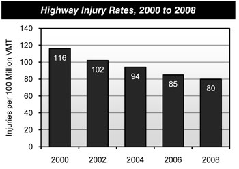
The overall number of traffic-related injuries has decreased over time, from about 3.1 million in 2000 to about 2.3 million in 2008. In 2000, the injury rate was 116 per 100 million VMT; by 2008, the number had dropped to 80 per 100 million VMT.
Chapter 5
Safety: Transit
Public transit in the United States has been and continues to be a highly safe mode of transportation, as evidenced by the statistics on incidents, injuries, and fatalities that have been reported by transit agencies for the vehicles they operate directly. Reportable safety incidents include collisions and any other type of occurrence that results in death, a reportable injury, or property damage in excess of a threshold. Since 2002, an injury has been reported only when a person has been immediately transported away from the scene of a transit incident for medical care. Any event producing a reported injury is also reported as an incident. Injuries and fatalities include those suffered by riders as well as by pedestrians, bicyclists, and people in other vehicles. Reportable security incidents include a number of serious crimes (robberies, aggravated assaults, etc.), as well as arrests and citations for minor offenses (fare evasions, trespassings, other assaults, etc.). Injuries and fatalities may occur not only while traveling on a transit vehicle, but also while boarding, alighting, or waiting for a transit vehicle or as a result of a collision with a transit vehicle or on transit property.
The definition of transit-related fatalities has remained the same. Non-homicide/non-suicide fatalities decreased from 245 in 2000 to 216 in 2008, and dropped from 0.56 per 100 million passenger miles traveled (PMT) in 2000 to 0.42 per 100 million PMT in 2008. Both the fatalities for 2008 and the rate per 100 million passenger miles demonstrate that transit is an extremely safe mode of transportation. With the fatality count steadily trending down since 2002, it experienced an unexplained increase of 30 deaths in 2007.
Data on incidents (safety and security combined) and injuries per 100 million PMT for transportation services on the five largest modes from 2004 to 2008 (excluding suicides and homicides) suggests that the highway modes (motor bus and demand response) became significantly safer in 2007 and 2008; however, given this dramatic decrease is unexplained, the data for these years may also suggest a reporting inconsistency. Data for the rail modes is volatile, but does not suggest any significant positive or negative trends over this period.
Although commuter rail has a very low number of incidents per PMT, commuter rail incidents are far more likely to result in a fatality than incidents occurring on any other mode. Most likely, this is because the average speed of commuter rail vehicles is considerably higher than the other rail modes (except vanpools). Motor buses, on the other hand, have a high number of incidents per PMT, but a lower chance of having an incident result in a fatality than almost any other mode (perhaps related to their low average speed).
| Year | Fatality Count | Fatalities per 100 Million PMT |
|---|---|---|
| 2000 | 245 | 0.56 |
| 2001 | 236 | 0.52 |
| 2002 | 249 | 0.55 |
| 2003 | 224 | 0.50 |
| 2004 | 217 | 0.48 |
| 2005 | 214 | 0.47 |
| 2006 | 213 | 0.44 |
| 2007 | 243 | 0.48 |
| 2008 | 216 | 0.42 |
| Analysis Parameter | 2004 | 2005 | 2006 | 2007 | 2008 |
|---|---|---|---|---|---|
| Incidents per 100 Million PMT | |||||
| Motor Bus | 77 | 74 | 79 | 66 | 54 |
| Heavy Rail | 45 | 40 | 42 | 43 | 53 |
| Commuter Rail | 20 | 22 | 19 | 18 | 16 |
| Light Rail | 63 | 67 | 62 | 61 | 48 |
| Demand Response | 895 | 1,010 | 1,298 | 247 | 204 |
| Injuries per 100 Million PMT | |||||
| Motor Bus | 76 | 70 | 71 | 69 | 67 |
| Heavy Rail | 33 | 26 | 32 | 31 | 43 |
| Commuter Rail | 17 | 21 | 17 | 18 | 16 |
| Light Rail | 42 | 37 | 36 | 44 | 48 |
| Demand Response | 449 | 506 | 729 | 227 | 234 |
Chapter 6
Finance: Highways
All levels of government combined generated $192.7 billion in 2008 to fund spending on highways and bridges; actual cash expenditures for highways and bridges were lower, totaling $182.1 billion in 2008. (The difference reflects amounts placed in reserve for expenditures in future years.)
Cash outlays by the Federal government for highway-related purposes were $40.0 billion (22.0 percent of the combined total), including both direct highway expenditures and amounts transferred to State and local governments for use on highways. States provided $90.6 billion (49.7 percent). Counties, cities, and other local government entities funded $51.5 billion (28.3 percent).
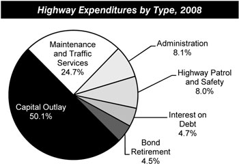
Of the total $182.1 billion spent for highways in 2008, $91.1 billion (50.1 percent) was used for capital investment. Spending on routine maintenance and traffic services totaled $44.9 billion (24.7 percent); administrative costs (including planning and research) were $14.7 billion; $14.6 billion was spent on highway patrol functions and safety programs; $8.5 billion was used to pay interest; and $8.2 billion was used for bond retirement.
Total highway expenditures by all levels of government increased by 48.4 percent between 2000 and 2008. Local government spending grew more quickly than Federal or State spending over this period; the share of total expenditures funded by the Federal government declined from 22.4 percent in 2000 to 22.0 in 2008. Federal cash expenditures for capital purposes outlay grew by 48.6 percent, from $26.1 billion in 2000 to $37.8 billion in 2008, while combined State and local capital investment increased by 51.5 percent. Consequently, the Federally-funded share of total capital outlay declined over this period (from 42.6 percent to 41.5 percent).
Of the total $82.7 billion of capital spending by all levels of government in 2008, $46.6 billion (51.1 percent) was used for system rehabilitation (resurfacing or replacing existing pavements and rehabilitating or replacing existing bridges). An estimated $33.6 billion (36.8 percent) was used for system expansion (constructing new roads and bridges or adding lanes to existing roads); and $11.0 billion (9.0 percent) went for system enhancements such as safety, operational, or environmental enhancements.
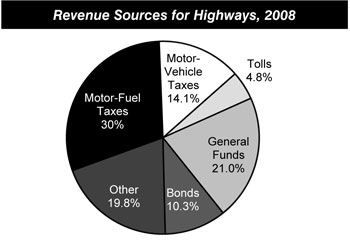
In 2008, $94.2 billion (48.9 percent) of the revenue generated for spending on highways and bridges came from highway-user charges—including motor-fuel taxes, motor-vehicle fees, and tolls. Other major sources of revenues for highways included general fund appropriations of $40.4 billion (21.0 percent) and bond proceeds of $19.9 billion (10.3 percent). All other sources such as property taxes, other taxes and fees, lottery proceeds, interest income, and miscellaneous receipts totaled $38.2 billion (19.8 percent).
Chapter 6
Finance: Transit
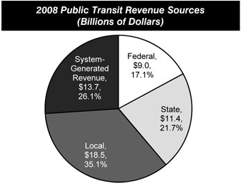
In 2008, $52.5 billion was generated from all sources to finance transit investment and operations. Transit funding comes from public funds allocated by Federal, State, and local governments and system-generated revenues earned by transit agencies from the provision of transit services. Of the funds generated in 2008, 73.9 percent ($38.8 billion) came from public sources and 26.1 percent came from passenger fares ($11.4 billion) and other system-generated revenue sources ($2.3 billion). The Federal share of this was $9.0 billion (23.1 percent of total public funding and 17.1 percent of all funding). Local jurisdictions provided the bulk of transit funds, $18.5 billion in 2008, or 47.5 percent of total public funds and 35.1 percent of all funding.
In 2008, total public transit agency expenditures for capital investment were $16.1 billion and accounted for 41.5 percent of total available funds. Federal funds were $6.4 billion in 2008, 39.8 percent of total transit agency capital expenditures. State funds provided an additional 12.4 percent and local funds provided the remaining 47.8 percent of total transit agency capital expenditures. Of total 2008 transit capital expenditures, 76.4 percent ($12.3 billion) was invested in rail modes of transportation, compared with 23.6 percent ($3.8 billion) invested in nonrail modes. This investment distribution has been consistent over the last decade.
| Transit Mode | Expenditure | Percent of Total |
|---|---|---|
| Rail | $12,292.5 | 76.4% |
| Commuter Rail | $2,686.2 | 16.7% |
| Heavy Rail | $6,125.8 | 38.1% |
| Light Rail | $3,458.3 | 21.5% |
| Other Rail | $22.2 | 0.1% |
| Nonrail | $3,796.3 | 23.6% |
| Motor Bus | $3,355.3 | 20.9% |
| Demand Response | $263.9 | 1.6% |
| Ferryboat | $113.2 | 0.7% |
| Trolley Bus | $44.6 | 0.3% |
| Other Nonrail | $19.3 | 0.1% |
| Total | $16,088.8 | 100.0% |
In 2008, $36.4 billion was available for transit operating expenses (wages, salaries, fuel, spare parts, preventive maintenance, support services, and leases). The Federal share of this has declined from the 2006 high of 8.2 percent to 7.1 percent. Similarly, the share generated from system revenues has decreased from 40.3 percent in 2006 to 37.6 percent. These decreases have been offset by the State share, which has increased from 22.5 percent in 2006 to 25.8 percent. The local share of operating expenditures has been close to 2008’s 29.7 percent for several years.
The average annual increase in operating expenditures per vehicle revenue mile for all modes combined between 2000 and 2008 was 4.1 percent. In 2008, the average operating expenditure across all transit modes was $8.60 per vehicle revenue mile. Analysis of National Transit Database reports for the largest 10 transit agencies (by ridership) shows that the growth in operating expenses is led by the cost of fringe benefits (36.0 percent of all operating costs for these agencies), which have been going up at a rate of 3.4 percent per year above inflation (constant dollars) since 2000. By comparison, average salaries at these ten agencies grew at an inflation-adjusted rate of only 0.1 percent per year in that period. Operating expenditures per passenger mile for all transit modes combined increased at an average annual rate of 4.3 percent between 2000 and 2008 (from $0.44 to $0.62).
Part II
Investment/Performance Analysis
The methods and assumptions used to analyze future highway, bridge, and transit investment scenarios for this report have evolved over time, to incorporate current research, new data sources, and improved estimation techniques relying on economic principles.
Traditional engineering-based analytical tools focus mainly on estimating transportation agency costs and the value of resources required to maintain or improve the conditions and performance of infrastructure. This type of analytical approach can provide valuable information about the cost effectiveness of transportation system investments from the public agency perspective, including the optimal pattern of investment to minimize life-cycle costs. However, this approach does not fully consider the potential benefits to users of transportation services from maintaining or improving the conditions and performance of transportation infrastructure.
The investment/performance analyses presented in Chapters 7 through 10 were developed using the Highway Economic Requirements System (HERS), the National Bridge Investment Analysis System (NBIAS), and the Transit Economic Requirements Model (TERM). Each of these tools has a broader focus than traditional engineering-based models and takes into account the value of services that transportation infrastructure provides to its users as well as some of the impacts of transportation activity on non-users. The methodologies used to analyze investment for highways, bridges, and transit are detailed in Appendices A, B, and C.
For purposes of computing a benefit-cost ratio for a transportation project, the “cost” (the denominator) is conventionally measured as the capital expenditures required to carry out the project. The “benefits” (the numerator) are generally measured in terms of reductions in costs experienced by (1) transportation agencies (such as for maintenance), (2) users of the transportation system (such as savings in travel time or vehicle operating costs, or reductions in crashes), and (3) others who are affected by the operation of the transportation system (such as reductions in environmental or other societal costs). Increases in any of these types of costs are treated as negative benefits.
An economics-based approach will likely result in different decisions about the catalog of desirable improvements than would a purely engineering-based approach. For example, if a highway segment, bridge, or transit system is greatly underutilized, benefit-cost analysis might suggest that it would not be worthwhile to fully preserve its condition or to address its engineering deficiencies. Conversely, a model based on economic analysis might recommend additional investments to expand capacity or improve travel conditions above and beyond the levels dictated by an analysis that simply minimized engineering life-cycle costs, if doing so would provide sufficient benefits to the users of the system. These types of considerations can potentially influence the establishment of standards as to what constitutes a “State of Good Repair” for different types of transportation assets.
An economics-based approach also provides a more sophisticated method for prioritizing potential improvement options when funding is constrained. By ranking investment opportunities in order of their benefit-cost ratios, economic analysis helps provide guidance in directing limited resources toward those improvements that provide the largest benefits to transportation system users. Projects selected for implementation can be limited to those having a benefit-cost ratio above the threshold that would result in all available funds being used; projects that produce lesser net benefits can be deferred for future consideration.
HERS, NBIAS, and TERM each use benefit-cost analysis as part of their decision-making process, but their approaches are very different. Each model relies on separate databases, making use of specific data available for only one part of the transportation network and addressing issues unique to that particular mode. The models have not evolved to the point where direct multimodal analysis is possible.
Chapter 7 analyzes the projected impacts of different levels of future capital investment on a series of measures of physical condition, operational performance, and other benefits to system users. These levels are described in terms of both average annual investment levels over 20 years, and the annual rate of increase or decrease in constant dollar investment that could generate these levels.
Chapter 8 presents a set of illustrative 20-year capital investment scenarios building upon the analysis presented in Chapter 7. The Department does not endorse or recommend any particular scenario. The investment levels associated with each scenario represent hypothetical levels of combined capital spending nationwide; the scenarios do not identify how much might be contributed by each level of government or from private sources to support such spending.
Some of these scenarios are oriented toward achieving a particular level of system performance. In considering the future system performance impacts identified for each scenario, it is important to note that they represent hypothetical models of what could be achievable assuming a particular level of investment rather than what would be achieved in reality. While the economics-based approach applied in HERS, NBIAS, and TERM would suggest that projects be implemented in order based on their benefit-cost ratios until the funding available under a given scenario is exhausted, the reality is that other factors influence Federal, State, and local decision making. If some projects with lower benefit-cost ratios were carried out in favor of projects with higher benefit-cost ratios, then the actual amount of investment required to achieve any given level of performance would be higher than the amount predicted in this report. Further, several assumptions, estimates, and projections are used to derive the investment scenarios and no effort to assess the predictive value of these models has been undertaken to date. As in any modeling process, simplifying assumptions have been adopted to make analysis practical and report within the limitations of available data.
Other scenarios are defined around funding all potential investments above a specified benefit-cost ratio threshold. It is important to note that simply increasing spending to the levels identified in these scenarios would not in itself guarantee that these funds would be expended in a cost-beneficial manner. Also, some potential capital investments selected by the models may be infeasible as a practical matter due to factors beyond those considered in the models. Because of this, the supply of feasible cost-beneficial projects could be exhausted at a lower level of investment than that indicated by these scenarios, and the projected improvements to future conditions and performance associated with these scenarios may not be fully obtainable in practice.
Chapter 9 provides supplemental scenario analyses, including comparisons of recent system performance and funding trends with projected future needs in order to identify consistencies and inconsistencies between what has occurred in the past and what is expected for the future. In addition, projections from selected prior editions are compared with actual spending and outcomes over time. Issues relating to the interpretation of scenarios, including the timing of future investment and the conversion of scenarios from constant dollars to nominal dollars, are also explored.
Chapter 9 includes a set of supplemental analyses that assume that any increases in highway and bridge spending above 2008 levels would be funded from user charges imposed on either a per-mile or a per-gallon basis. The general effect of such charges is to reduce future travel and reduce the projected level of investment needed to achieve a particular performance objective. These analyses also examine the potential impacts that the widespread adoption of congestion pricing might be expected to have on the level of investment required to achieve certain levels of future conditions and performance.
Chapter 10 explores the impact that changing some key technical assumptions could have on the overall results projected by HERS, NBIAS, and TERM.
Chapter 7
Potential Capital Investment Impacts: Highways and Bridges
Of the $91.1 billion of total capital outlay by all levels of government combined in 2008, $54.7 billion was used for types of capital improvements modeled in HERS, including pavement resurfacing, pavement reconstruction, and system expansion. (HERS models investments on Federal-aid highways only; $12.7 billion was spent on similar types of improvements to other roads.) In 2008, $12.8 billion was spent on improvement types modeled in NBIAS, including bridge repair, rehabilitation, and replacement. The remaining $11.0 billion went for system enhancements not captured by either model.
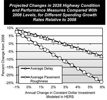
Sustaining HERS-modeled capital spending on Federal-aid highways at its base year 2008 level in constant dollar terms for 20 years (i.e., an annual change in spending of zero percent) is projected to result in a worsening of overall system performance in 2028 relative to 2008, including a 2.8 percent increase in pavement roughness, and a 6.7 percent increase in average delay per VMT; if annual spending growth were negative, HERS projects even larger increases in pavement roughness and delay by 2028.
HERS projects that if constant dollar spending were to grow by 5.90 percent per year, this would be sufficient to finance all potentially cost-beneficial capital improvements on Federal-aid highways by 2028; at this level of investment, average pavement roughness and delay are projected to improve by 24.3 percent and 7.7 percent, respectively, over the period 2008 through 2028.
The NBIAS model estimates that there was a backlog of potentially cost-beneficial bridge investments in 2008 of $121.2 billion, of which $102.1 billion was on Federal-aid highway bridges, $60.4 billion was on NHS bridges, and $38.1 billion was on Interstate System bridges. (These figures do not include costs associated with system expansion modeled separately in HERS.) In the absence of future capital investment, this backlog would grow over time as existing bridges age.
If spending by all levels of government for the types of improvements modeled in NBIAS were sustained at 2008 levels ($12.8 billion—all bridges; $9.4 billion—Federal-aid highway bridges; $5.4 billion—NHS bridges; $3.3 billion—Interstate System bridges) in constant dollar terms, NBIAS projects that this would be sufficient to reduce the backlog by 2028 for Interstate System bridges, NHS bridges, and all bridges; however, the backlog for Federal-aid highway bridges would increase by an estimated 6.5 percent, driven primarily by the subset of bridges on Federal-aid highways that are not on the NHS.
| System Subset | 2008 Bridge Backlog (Billions of 2008 Dollars) | Percent Change by 2028 |
|---|---|---|
| Interstate Bridges | $38.1 | -3.6% |
| NHS Bridges | $60.4 | -1.8% |
| Federal-Aid Highway Bridges | $102.1 | 6.5% |
| All Bridges | $121.2 | -11.2% |
NBIAS projects that eliminating the economic bridge investment backlog and addressing new bridge deficiencies as they arise over 20 years would require an annual increase in constant dollar spending of 4.31 percent for all bridges, 5.36 percent for Federal-aid highway bridges, 4.48 percent for NHS bridges, and 4.39 percent for Interstate System bridges.
Chapter 7
Potential Capital Investment Impacts: Transit
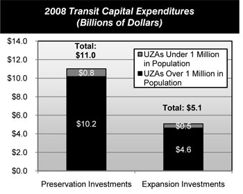
U.S. transit agencies spent a combined $16.1 billion in 2008 on capital improvements to the Nation’s transit infrastructure and vehicle fleets. This amount included $11.0 billion in the preservation (rehabilitation and replacement) of existing assets already in service and $5.1 billion to expand transit capacity—both to accommodate ridership growth and to improve performance for existing riders.
Sustaining TERM-modeled transit capital spending at these base year 2008 levels for 20 years is projected to result in an overall decline in both transit system conditions and performance. This includes an overall deterioration in the average physical condition of the Nation’s stock of transit assets, with consequent performance impacts on service reliability and potentially on safety, an estimated 50 percent increase in the size of the “State of Good Repair” (SGR) backlog by 2030, and increases in vehicle crowding on the order of 5 to 30 percent (depending on the magnitude of ridership growth).
For this edition of the report, the FTA developed an SGR benchmark scenario which estimates the investment required to attain and maintain a state of good repair for the Nation’s existing transit assets. Prior editions of this report included scenarios that were based on maintaining conditions or improving the condition of assets. Details of the new scenarios relative to past scenarios are provided in Chapter 9 and its Executive Summary.
Accordingly, for the SGR benchmark scenario, TERM estimates the average annual level of 20-year investment required to eliminate the existing investment backlog and bring all existing transit assets to the SGR benchmark to be roughly $18.0 billion (without consideration of investment cost-effectiveness) and closer to $17.0 billion if limited to those asset reinvestments passing TERM’s cost-benefit analysis. Similarly, an additional $4.2 billion to $7.3 billion in annual expansion investments are required to maintain transit performance (as measured by vehicle crowding) at 2008 levels, depending on the actual rate of growth in ridership.
When limited to urbanized areas (UZAs) with populations greater than 1 million, transit agencies expended $14.8 billion on capital projects in 2008, including $10.2 billion on asset preservation and $4.6 billion on transit capacity expansion. In contrast, the average annual investment level for these UZAs to attain SGR is estimated to be $15.6 billion over the next 20 years (without consideration of investment cost effectiveness) and closer to $14.5 billion to $15.1 billion if limited to those asset reinvestments passing TERM’s cost-benefit analysis. These scenarios suggest that an additional $2.6 billion to $6.1 billion are required to support projected increases in transit boardings while maintaining current service performance levels (as measured by the number of riders per peak vehicle).
Transit agencies operating outside of UZAs with populations greater than 1 million expended $1.3 billion on capital projects in 2008, including $0.8 billion on preservation and $0.5 billion on asset expansion. In contrast, the average annual investment level for these smaller UZAs and all rural areas to attain SGR is estimated to be $2.4 billion over the next 20 years (or approximately $2.0 billion if limited to those reinvestments passing TERM’s benefit-cost analysis), while the level of average annual investment required to address both SGR and asset expansion needs of these smaller UZAs and rural areas is estimated to be between $2.5 billion and $2.8 billion, depending on the level of ridership growth.
Chapter 8
Selected Capital Investment Scenarios: Highways
This report presents a set of illustrative 20-year capital investment scenarios; this report does not endorse any of these scenarios as a target level of funding, nor does it make any recommendations concerning future levels of Federal funding. The scenarios for highways and bridges build upon separate analyses developed using HERS and NBIAS and take into account other types of capital spending that are not currently modeled. The scenario criteria were applied separately to the Interstate System, the NHS, Federal-aid highways, and the highway system as a whole.
The Sustain Current Spending scenario assumes that capital spending is sustained in constant dollar terms at base year 2008 levels between 2009 and 2028. (In other words, spending would rise by exactly the rate of inflation over that period).
The Maintain Conditions and Performance scenario assumes that capital investment gradually changes in constant dollar terms over 20 years to the point at which selected measures of highway and bridge performance in 2028 are maintained at their base year 2008 levels. The average annual investment levels associated with meeting these goals are $24.3 billion for the Interstate System, $38.9 billion for the NHS, $80.1 billion for Federal-aid highways, and $101.0 billion for all roads. The cost to maintain value identified for the NHS is lower than the $42.0 billion spent by all levels of government combined on the NHS in 2008, indicating that sustaining NHS spending at 2008 levels could result in improved overall conditions and performance on the NHS.
The Improve Conditions and Performance scenario assumes that capital investment gradually rises in constant dollar terms to the point at which all potentially cost-beneficial investments could be implemented by 2028. This scenario can be thought of as an “investment ceiling” above which it would not be cost-beneficial to invest. The average annual investment level for this scenario is $170.1 billion for all roads, 86.6 percent higher than actual spending in 2008.
| System Subset | Sustain Current Spending | Maintain Conditions and Performance | Improve Conditions and Performance |
|---|---|---|---|
| Interstate | $20.0 | $24.3 | $43.0 |
| NHS | $42.0 | $38.9 | $71.8 |
| Federal-Aid Highways | $70.6 | $80.1 | $134.9 |
| All Roads | $91.1 | $101.0 | $170.1 |
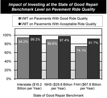
Of the $170.1 billion Improve Conditions and Performance scenario investment level for all roads, $85.1 billion (50 percent) would be directed toward improving the physical condition of existing infrastructure assets; this amount is identified as the State of Good Repair benchmark. The average annual State of Good Repair benchmark levels identified for Federal-aid highways, the NHS, and the Interstate System are $67.8 billion, $29.8 billion, and $16.2 billion, respectively. Investing at these levels could bring the share of Federal-aid highway VMT on pavements with good ride quality up from 46.4 percent in 2008 to 74.1 percent by 2028; the comparable percentages for the NHS and the Interstate System could be increased to 89.6 percent and 94.2 percent, respectively, by 2028. HERS projects that improving these measures beyond this point would not be cost-beneficial.
Chapter 8
Selected Capital Investment Scenarios: Transit
This report presents a set of illustrative 20-year transit capital investment scenarios. The scenarios for transit capital needs build upon analyses developed using TERM and were applied separately to the Nation’s transit assets as a whole, as well as for two separate groupings of transit operators based on the size of the UZAs they serve.The Sustain Current Spending scenario assumes that capital spending is sustained in constant dollar terms at year 2008 levels between 2009 and 2028. Transit operators spent $16.1 billion on capital projects in 2008. Of this amount, $11.0 billion was devoted to the preservation of existing assets while the remaining $5.1 billion was dedicated to investment in asset expansion to support ongoing ridership growth and to improve service performance. This scenario considers the expected impact on the physical conditions and performance of the Nation’s transit infrastructure if these expenditure levels are sustained in constant dollar terms. TERM analysis suggests that sustaining spending at 2008 levels would likely yield an overall decline in transit conditions, an estimated 50 percent increase in the SGR backlog by 2030, and an increase in crowding on transit passenger vehicles.
The State of Good Repair (SGR) benchmark estimates the level of annual capital investment required to eliminate the current transit investment backlog and then maintain all transit assets in a state of good repair thereafter, all without consideration of the cost-effectiveness of each investment (i.e., investments are not required to pass TERM’s benefit-cost test under this scenario). TERM estimates this annual level of investment to be $18.0 billion for the Nation as a whole. This includes $15.6 billion for UZAs with populations greater than 1 million (with most of these funds required for rail asset reinvestment), and $2.4 billion for the remaining smaller UZAs and rural areas currently served by transit.
The Low Growth and High Growth scenarios consider the level of investment to address both asset SGR and service expansion needs subject to two differing potential levels of growth (and with all investments now required to pass a benefit-cost analysis). The Low Growth scenario assumes transit ridership will grow as projected by the Nation’s metropolitan planning organizations (MPOs), while the High Growth scenario assumes the average rate of growth (by UZA) as experienced in the industry since 1999. The Low Growth scenario assumes that ridership will grow at an annual rate of 1.4 percent over the 20-year period from 2008 to 2028; conversely, the High Growth scenario assumes that ridership will increase at a rate of 2.8 percent per year over that time frame. TERM estimates this average annual level of investment to be between $20.8 billion and $24.5 billion for the Nation as a whole between 2008 and 2028, including from $16.6 billion to $17.2 billion for asset preservation and $4.2 billion to $7.3 billion for expansion needs, depending on the realized rate of ridership growth.
When limited to the UZAs with populations greater than 1 million, the average annual level of investment to address both SGR and expansion needs is $18.2 billion to $21.7 billion. The comparable range for the smaller UZAs and all rural areas with transit is $2.5 billion to $2.8 billion annually.
| Mode and Asset Type | Investment (Billions of 2008 Dollars) SGR |
Investment (Billions of 2008 Dollars) Low Growth |
Investment (Billions of 2008 Dollars) High Growth |
|---|---|---|---|
| UZAs Over 1 Million in Population | |||
| Nonrail | $4.9 | $5.6 | $6.9 |
| Rail | $10.7 | $12.7 | $14.8 |
| Total* | $15.6 | $18.2 | $21.7 |
| UZAs Under 1 Million in Population and Rural | |||
| Nonrail | $2.1 | $2.4 | $2.6 |
| Rail | $0.3 | $0.2 | $0.2 |
| Total* | $2.4 | $2.5 | $2.8 |
| Total* | $18.0 | $20.8 | $24.5 |
Chapter 9
Supplemental Scenario Analysis: Highways
As noted earlier, Chapter 8 includes scenarios for selected subsets of the overall highway system. The particular analyses from Chapter 9 discussed below apply to Federal-aid highways only, not to all roads.
The goal of the Maintain Conditions and Performance scenario is to maintain overall conditions and performance for the lowest cost possible, without regard to how various system components might be affected. In practice, the conditions and performance of higher-ordered functional systems such as principal arterials tend to improve under this scenario, offset by some deterioration on lower-ordered systems. Maintaining pavement condition, bridge condition, and operational performance for each individual functional class would be more expensive. While the average annual investment level associated with the Maintain Conditions and Performance scenario for Federal-aid highways is $80.1 billion, maintaining these specific performance measures on individual functional systems would cost $88.8 billion per year.
| Functional System | Cost to Maintain System Components | Maintain Conditions and Performance Scenario |
|---|---|---|
| Rural Arterials and Major Collectors | ||
| Interstate | $4.2 | $4.5 |
| Other Principal Arterial | $4.2 | $4.0 |
| Minor Arterial | $5.0 | $3.4 |
| Major Collector | $7.7 | $4.4 |
| Subtotal | $21.1 | $16.2 |
| Urban Arterials and Collectors | ||
| Interstate | $18.7 | $23.5 |
| Other Freeway and Expressway | $7.9 | $10.1 |
| Other Principal Arterial | $16.8 | $12.7 |
| Minor Arterial | $15.4 | $12.4 |
| Collector | $8.9 | $5.1 |
| Subtotal | $67.7 | $63.9 |
| All Federal-Aid Highways | $88.8 | $80.1 |
The baseline scenarios presented in this report assume no linkages between future investment needs and the types of financing mechanisms that might be utilized to address those needs. In reality, increasing user charges to support additional future spending would have an impact on the cost of driving, and hence would affect future VMT growth. The widespread adoption of congestion pricing would have a particularly significant impact on future system performance and investment needs.
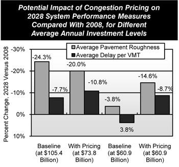
Of the average annual investment level associated with the Maintain Conditions and Performance scenario for Federal-aid highways, $60.9 billion was derived from HERS. At this level of investment, HERS projects that average pavement roughness would improve by 3.8 percent, while average delay per VMT would worsen by 3.8 percent. Assuming the widespread adoption of congestion pricing, the model predicts improvements of 14.6 percent in average pavement roughness and 8.7 percent in average delay. (Under this alternative, HERS changes its mix of spending in favor of pavements, resulting in improved pavement conditions.)
Of the $134.9 billion average annual investment level for the Improve Conditions and Performance scenario for Federal-aid highways, $105.4 billion was derived from HERS; assuming the widespread adoption of congestion pricing, HERS projects that an average annual investment level of only $73.8 billion would be needed to address all potentially cost-beneficial improvements.
Chapter 9
Supplemental Scenario Analysis: Transit
Prior editions of this report included scenarios that considered the level of investment required either to (1) maintain the condition of existing transit assets at current levels or to (2) improve the condition of those assets to an overall condition of “good” (i.e., 4.0 on TERM’s condition scale). For this edition, these “maintain” and “improve” conditions scenarios have been replaced by the SGR benchmark, which estimates the investment required to attain and maintain a state of good repair for the Nation’s existing transit assets. The SGR benchmark is financially unconstrained and considers the level of investment required to eliminate the current investment backlog and to address all reinvestment needs as they arise such that all asset conditions remain at 2.5 or higher on TERM’s condition scale. This change was found to have two key implications.
First, analysis has determined that, given a high proportion of existing long-lived assets currently in good or excellent condition, it is not realistic or rational to attempt to maintain asset conditions at current levels over the next 20 years. Assuming transit operators follow reasonable asset rehabilitation and replacement policies, asset conditions are likely to decline (even as the proportion of assets not in SGR is reduced) until existing transit assets attain a “steady state” average condition value that reflects a given set of rehabilitation and replacement practices.
Second, only a significant and ongoing investment in expansion assets can reverse this general downward trend in conditions. Moreover, it is just this type of ongoing expansion in new transit assets over the past two decades that has tended to reduce the rate of decline in average conditions across all transit assets (both new and existing). Analysis suggests that this effect has tended to mask somewhat the underlying decline in asset conditions for existing (as opposed to existing plus new) transit assets.
Also in contrast to prior report editions, which only considered a single ridership growth projection, this edition assesses transit capital expansion under both low and high ridership growth outcomes. Specifically, the Low Growth scenario assumed UZA-specific rates of PMT growth projected by the Nation’s MPOs, while the High Growth scenario assumed the UZA-specific average annual compound rates based on historical growth rate averages.
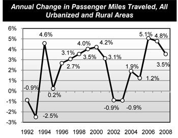
Analysis shows that historical rates of PMT growth have typically exceeded the MPO-projected rates of growth typically used for long-range transportation planning purposes. (In the past, the MPO-projected rates have been the only source of ridership growth estimates used to generate transit expansion needs in prior editions of this report.) For example, from 1992 to 2008, the historical compound annual PMT growth rate averaged roughly 2.1 percent compared with the 1.3 percent growth rate MPOs have projected for the upcoming 20-year period.
Given the difference between the two growth rates (and the relatively high rate of historic PMT growth as compared with other measures, such as UZA population growth), the 2.1 percent historical growth rate of PMT was identified as a reasonable input value for the High (or higher) Growth scenario. Similarly, the 1.3 percent MPO-projected growth rate was used as an input value for the Low (or lower) Growth scenario.
Chapter 10
Sensitivity Analysis: Highways and Bridges
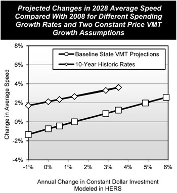
States provide forecasts of future VMT for each individual HPMS sample section evaluated in HERS; for 2008, the weighted average annual VMT growth rate based on these forecasts is 1.85 percent. HERS assumes that these forecasts represent the annual growth in travel over 20 years that would occur if a constant level of service is maintained on that facility. This assumption is reflected in the baseline analysis presented in this report, for which HERS estimates that an annual constant dollar spending increase of 5.90 percent could be sufficient to fund all potentially cost-beneficial investments by 2028, translating into an average annual investment level of $105.4 billion (compared with the $54.7 billion spent in 2008 on the types of capital spending modeled in HERS).
To explore the possibility that traffic might grow more slowly than assumed, an alternative HERS analysis was conducted assuming for illustration that VMT will grow at the average annual rate of 1.23 percent, the historical average from 1998 to 2008. Modifying the input forecasts to match this VMT growth rate would reduce the benefits associated with pavement and capacity improvements, so that an annual spending increase of only 3.52 percent (translating into an average annual investment level of $80.2 billion) would be sufficient to fund all potentially cost-beneficial projects by 2028. If spending were instead sustained at 2008 levels, HERS projects that average speeds would improve by 2.1 percent under this alternative compared with a decline of 0.7 percent under the baseline assumptions.
Another sensitivity test concerns the growth rate between 2008 and 2028 in motor fuel prices relative to general rate of inflation. The baseline HERS assumption is of no difference between these rates. An alternative assumption was based on the High Oil Price case from the Energy Information Administration, Annual Energy Outlook 2010. In this case, the ratio of gasoline prices to the consumer price index nearly regains its 2008 level by 2012 and increases thereafter through 2028 at the equivalent of 3.4 percent annually. The change in assumption from the baseline case causes HERS to reduce its projection of future travel growth and reduces the model’s estimate of the average annual investment level needed to fund all projects with a benefit-cost ratio of 1.0 or higher by 2028 to $96.9 billion.
Increases in travel time clearly impose costs on drivers, but it is difficult to precisely quantify the value of time, much less forecast changes. Increasing the baseline estimate of the value of time by 25 percent would cause HERS to attribute more benefits to projects (particularly widening projects) that would result in travel time savings. This in turn would increase the estimate of potentially cost-beneficial investment to $114.0 billion per year.
The HERS and NBIAS models each apply a discount rate to future benefits to reflect the implicit cost associated with directing resources to improve highways or bridges that could otherwise be used elsewhere in the public or private sector. Reducing the discount rate from the baseline 7 percent to 3 percent (reflecting lower interest rates) would increase the HERS estimate of the average annual investment level needed to fund all potentially cost-beneficial projects to $129.0 billion. The comparable average annual investment level projected by NBIAS for all bridges would be $24.8 billion assuming a 3 percent discount rate, about 21 percent more than the $20.5 billion baseline value computed based on a 7 percent discount rate.
Chapter 10
Sensitivity Analysis: Transit
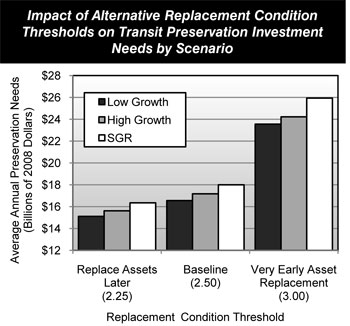
TERM relies on a number of key input values, variations of which can significantly impact the value of TERM’s capital needs projections. Each of the three unconstrained investment scenarios examined in Chapter 8—including the SGR benchmark and the Low Growth and High Growth scenarios—assumes that assets are replaced at a condition rating of 2.50 as determined by TERM’s asset condition decay curves. Analysis suggests that each of these scenarios is sensitive to changes in this replacement condition threshold, with the sensitivity increasing disproportionally the higher the replacement condition threshold is increased. For example, reducing the condition threshold to 2.25 tends to reduce preservation needs by just under $2 billion (close to 10 percent). In contrast, increasing the threshold to 2.75 increases preservation needs by more than $3 billion (just under 20 percent), while a further threshold increase to 3.00 increases preservation needs by nearly $8 billion (over 40 percent). This increasing sensitivity reflects the fact that ongoing, equal incremental changes to the replacement condition threshold yield greater proportionate reductions in the length of the asset life cycles as higher replacement condition values are reached.
Needs estimates for scenarios employing TERM’s benefit-cost analysis are also particularly sensitive to changes in capital costs (assuming no comparable increase in benefits), as these increases tend to reduce the value of the benefit-cost ratio, causing some previously acceptable projects to fail this test. For example, a 25 percent increase in capital costs increases investment costs by just under $3 billion (nearly 14 percent) for the Low Growth scenario and by just under $4 billion (over 15 percent) for the High Growth scenario. In contrast, needs under the SGR benchmark (which does not utilize TERM’s benefit-cost test) increase by more than $4 billion (precisely 25 percent) in response to a 25 percent increase in capital costs.
The most significant source of transit investment benefits as assessed by TERM’s benefit-cost analysis is the net cost savings to users of transit services, a key component of which is the value of travel time savings. Consequently, the per-hour value of travel time for transit riders is a key driver of total investment benefits for scenarios that employ TERM’s benefit-cost test. For example, a doubling of the value of time increases total needs for the Low Growth and High Growth scenarios by approximately $2 to $3 billion (8 to 10 percent) due to the increase in total benefits relative to costs. Similarly, a halving of the value of time decreases total investment needs for these scenarios by approximately $3 billion each (12 to 14 percent.
Finally, TERM’s benefit-cost test is responsive to the discount rate used to calculate the present value of the streams of investment costs and benefits. For example, reducing the discount rate from the base rate of 7 percent to 3 percent yields approximately $1 to $2 billion (6 to 8 percent) increase in total investment needs under the Low Growth and High Growth scenarios, respectively.
| Changes in Value of Time | Low Growth | High Growth |
|---|---|---|
| Reduce 50% ($5.60)* | $17.91 | $21.51 |
| Baseline ($11.20)* | $20.76 | $24.47 |
| Increase 100% ($22.40)* | $22.40 | $26.99 |
| Inflate to 2008 Dollars ($13.49) | $21.05 | $24.87 |
Chapter 11
Environmental Sustainability
The 1987 United Nations (UN) World Commission on Environment and Development defined sustainability as “development that meets the needs of the present without compromising the ability of future generations to meet their own needs.” While other organizations have defined sustainability differently, a common concept that has emerged is the “triple bottom line,” referring to the economy, the environment, and society. In transportation, the triple bottom line relates to sustainable solutions for the natural environmental systems surrounding the transportation system, the economic efficiency of the system, and societal needs (e.g., mobility, accessibility, and safety).
Transportation is crucial to our economy and quality of life, but the process of building, operating, and maintaining transportation systems has environmental consequences. Fostering more environmentally sustainable approaches to transportation is essential in order to avoid negative impacts in the near term and to ensure that future generations will be able to enjoy the same or better standards of living and mobility as exist today. Sustainable transportation focuses on environmental impacts such as improved energy efficiency, reduced dependence on oil, reduced greenhouse gas (GHG) emissions, and other improvements to the natural environment involving air quality and water quality.
From a sustainability perspective, the heavy reliance of the transportation system on fossil fuels is of significant concern, as they are non-renewable; generate air pollution; and contribute to the buildup of carbon dioxide (CO2) and other GHGs, which trap heat in the Earth’s atmosphere. The United States has relatively high GHG emissions per capita, even compared with other similarly affluent countries. The transportation sector consumes 29 percent of the total energy used in the United States; this represents 5 percent of global GHG emission.
Over the past four decades, progress has been made in reducing emissions of air pollutants both nationally and from the transportation sector in particular. However, many Americans continue to live in regions that exceed health-based air-quality standards. To seek more sustainable options, transportation programs will need to focus on designing, constructing, maintaining, and operating infrastructure in ways that accommodate multiple modes of transportation, promote connectivity, and minimize environmental impacts.
Establishing Sustainability Goals
At this time there is no widely recognized and accepted method for measuring sustainability in the transportation community. One of the challenges is the need to shift from operations-focused performance measures to more holistic indicators, even if they are more difficult to quantify.
At the Federal level, environmental sustainability has been adopted as a strategic goal in the U.S. DOT Strategic Plan 2010-2015. At the State level, transportation agencies are developing metrics that address various aspects of sustainability and monitoring progress toward specific goals—often in their long-range and project-level planning process. Some potential measures that have been identified for assessing progress in improving sustainability relate to reducing GHG emissions, improving system efficiency, reducing the growth of VMT, transitioning to fuel-efficient vehicles and alternative fuels, and increasing the use of recycled materials in transportation.
Sustainability in Transportation Planning
The transportation planning process provides a forum for discussion of environmental, economic, and community concerns and can facilitate the inclusion of sustainability considerations into transportation projects. One example of efforts to respond to the challenge of creating a sustainable transportation system is the increased use of context sensitive solutions (CSS). A CSS approach requires that transportation planning consider the interaction between transportation systems and tailor them to the local area’s human, cultural, and natural environment.
Chapter 12
Climate Change Adaptation
Climate change has received increased attention over the last decade, with a key concern being the impact on people and the planet. For the transportation community, policies to address climate change focus on GHG mitigation and climate change adaptation. Climate change adaptation focuses on anticipating potential future changes (e.g., higher sea levels, increased temperatures, altered precipitation patterns, greater storm intensity) and the potential impact on transportation (e.g., damaged or flooded facilities).
Impacts of Climate Change Adaptation on Transportation
Research efforts regarding the potential impacts of climate change on highway infrastructure are ongoing. U.S. DOT released a report on projected changes in climate over the century, used geographical information systems to map areas with transportation infrastructure along the Atlantic coast that will be potentially vulnerable to sea level rise, and is conducting a second adaptation study focused on the Gulf Coast region. These studies identify potential climate change impacts that are widespread and modally diverse and that would stress transportation systems in ways beyond which they were designed.
Temperature and sea levels have risen in recent decades, and these rates of change may accelerate in the future as GHG concentrations rise. Climate change has the potential to cause real damage to transportation infrastructure and services.
Steps for Assessing Adaptation Needs
Transportation agencies across the Nation are addressing climate change mitigation issues at various levels; however, the issue of adapting transportation infrastructure to climate change impacts has received less widespread attention. Discussions to date have focused primarily on coastal States.
Adapting to the impacts of climate change starts with inventorying critical infrastructure, understanding potential future climate change impacts, and assessing vulnerabilities and risks.
Once adaptation needs are assessed, adaptation options can be classified in one of five broad categories. “Maintain, manage, and operate” strategies make no changes to the base transportation facility and focus on repairing damages as they occur. A “protect and strengthen” approach involves proactively strengthening a facility to meet new design standards that can withstand climate change effects. “Relocate and avoid” strategies move existing facilities to areas less threatened by climate change. An “abandon and disinvest” approach involves discontinuing service on facilities when it is no longer financially feasible to continue investment in them given current or potential threats. “Promote redundancy” strategies are aimed at adding assets that could serve as backup facilities if primary facilities fail.
Barriers to Action
A critical obstacle to creating adaptation strategies is the lack of adequate information on how and when the climate will change. Without this type of information, assessment of risk and designing development strategies are difficult. Transportation design, maintenance, and replacement will need to be more flexible to incorporate climate adaptation considerations.
Adaptation Activities
Adaptation activities are underway at both the Federal and State levels. The U.S. DOT is working to develop models to assess and identify climate change vulnerabilities and risks to critical transportation assets. Additional studies on regional impacts of climate changes are also in process. At the State level, climate change adaptation action plans to consider necessary adaptation and mitigation strategies are being developed by several States.
Chapter 13
Livability
Fostering livable communities—places where transportation, housing, and development have been coordinated to provide access to adequate, affordable, and environmentally sustainable transportation options—is a goal of the U.S. DOT.
Transportation plays an important role in creating safer, healthier communities with the strong economies needed to support our families.
A key component of livable communities is having transportation choices. A multimodal system that integrates walking, bicycling, transit, and automobile access provides residents with more choices of where to live, work, and play. Integrating land use planning with transportation improves livability by fostering a balance of mixed-use neighborhoods that recognizes the importance of proximity, layout, and design to help keep people close to home, work, services, and recreation.
Benefits of Livable Communities
The following are some of the many benefits to considering the role of transportation in creating livable communities:
- Provides more transportation options and integrates land use planning
- Promotes healthy living
- Improves pedestrian safety
- Proves popular with citizens
- Increases economic competitiveness
- Incentivizes business investment
- Lowers transportation costs
- Saves community infrastructure costs.
HUD/DOT/EPA Partnership
In June 2009, the U.S. DOT, HUD, and EPA initiated an Interagency Partnership for Sustainable Communities (Partnership) to improve access to affordable housing, provide more transportation options, and lower transportation costs while protecting the environment in communities nationwide. The Partnership established six livability principles as follows:
- Provide more transportation choices
- Promote equitable, affordable housing
- Enhance economic competitiveness
- Support existing communities
- Coordinate policies and leverage investment
- Value communities and neighborhoods.
Livability Performance Measures
Communities across the United States have begun tracking the implementation process and accessibility outcomes of livability investments that expand transportation options. However, it is easier to articulate the benefits of livable communities than to quantify them; work is continuing to reach a consensus in terms of what data should be collected on a consistent basis nationwide to track progress in improving livability.
Given the limitations of the data that are currently available, the U.S. DOT has identified some interim measures to begin tracking progress in meeting the goal of fostering livable communities. The President’s FY 2012 Budget includes the following measures and targets relating to livability:
- Increase the number of States with policies that improve transportation choices for walking and bicycling from 21 in 2010 to 23 in 2012.
- Increase access to convenient and affordable transportation choices as reflected by the average percentage change in transit boarding per transit market by 2.0 percent per year from 2010 to 2012.
- Improve access to transportation for special needs populations as reflected by the percentage of bus fleets compliant with the Americans with Disabilities Act (ADA) from 97 percent in 2007 to 98 percent in 2012 and increase the percentage of key rail stations that are ADA compliant from 93 to 95 percent between 2007 and 2012.