


- Potential Highway Capital Investment Impacts
- Types of Capital Spending Projected by HERS and NBIAS
- Alternative Levels of Future Capital Investment Analyzed
- Highway Economic Requirements System
- Impacts of Federal-Aid Highway Investments Modeled by HERS
- Impacts of NHS Investments Modeled by HERS
- Impacts of Interstate System Investments Modeled by HERS
- National Bridge Investment Analysis System
- Impacts of Systemwide Investments Modeled by NBIAS
- Impacts of Federal-Aid Highway Investments Modeled by NBIAS
- Impacts of NHS Investments Modeled by NBIAS
- Impacts of Interstate Investments Modeled by NBIAS
- Potential Transit Capital Investment Impacts
Potential Highway Capital Investment Impacts
The analyses presented in this section use a common set of assumptions to derive relationships between alternative levels of future highway capital investment and various measures of future highway and bridge conditions and performance. A subsequent section within this chapter provides comparable information for different types of potential future transit investments.
The analyses in this section focus on the types of investment within the scopes of the Highway Economic Requirements System (HERS) and the National Bridge Investment Analysis System (NBIAS), and form the building blocks for the capital investment scenarios presented in Chapter 8. The accuracy of the projections in this chapter depends on the validity of the technical assumptions underlying the analysis, some of which are varied in the sensitivity analysis in Chapter 10. The analyses presented in this section do not make any explicit assumptions regarding how future investment in highways might be funded.
Types of Capital Spending Projected by HERS and NBIAS
The types of investments evaluated by HERS and NBIAS can be related to the system of highway functional classification introduced in Chapter 2 and to the broad categories of capital improvements introduced in Chapter 6 (system rehabilitation, system expansion, and system enhancement). NBIAS relies on the NBI database, which covers bridges on all highway functional classes, and evaluates improvements that generally fall within the system rehabilitation category.
HERS evaluates pavement improvements—resurfacing or reconstruction—and highway widening; the types of improvements included in these categories roughly correspond to system rehabilitation and system expansion as described in Chapter 6. In estimating the per-mile costs of widening improvements, HERS recognizes a typical number of bridges and other structures that would need modification. Thus, the estimates from HERS are considered to represent system expansion costs for both highways and bridges. Coverage of the HERS analysis is limited, however, to Federal-aid highways, as the Highway Performance Monitoring System (HPMS) sample does not include data for rural minor collectors, rural local roads, or urban local roads.
The term “non-modeled spending” refers in this report to spending on highway and bridge capital improvements not evaluated in HERS or NBIAS; while these types of spending are absent from the analyses presented in this chapter, the capital investment scenarios presented in Chapter 8 are adjusted to account for them. Non-modeled spending includes capital improvements on highway classes omitted from the HPMS sample and hence the HERS model. Development of future investment scenarios for the highway system as a whole thus requires separate estimation outside the HERS modeling process.
Non-modeled spending also includes types of capital expenditures classified in Chapter 6 as system enhancements, which neither HERS nor NBIAS currently evaluate. Although HERS incorporates assumptions about future operations investments, whose capital components would be classified as system enhancements, the model does not directly evaluate the need for these deployments. In addition, HERS does not identify specific safety-oriented investment opportunities, but instead considers the ancillary safety impacts of capital investments that are directed primarily toward system rehabilitation or capacity expansion. This limitation of the model owes to the HPMS database containing no information on the location of crashes or of safety devices such as guardrails or rumble strips.
| How closely do the types of capital improvements modeled in HERS and NBIAS correspond to the specific capital improvement type categories presented in Chapter 6? | |
|
Exhibit 6-12 in Chapter 6 provides a crosswalk between a series of specific capital improvement types for which data are routinely collected from the States, and three major summary categories: system rehabilitation, system expansion, and system enhancement. The types of improvements covered by the HERS and NBIAS model are assumed to correspond with the system rehabilitation and system expansion categories. As in Exhibit 6-12, HERS splits spending on “reconstruction with added capacity” between these categories.
The assumed correspondence is close overall, but for some of the detailed categories in Exhibit 6-12 not exact. In particular, the extent to which HERS covers construction of new roads and bridges is ambiguous. While not directly modeled in HERS, such investments are often motivated by a desire to alleviate congestion on existing facilities in a corridor, and thus would be captured indirectly by the HERS analysis in the form of additional normal-cost or high-cost lanes. As described in Appendix A, the costs per mile assumed in HERS for high-cost lanes are based on typical costs of tunneling, double-decking, or building parallel routes, depending on the functional class and area population size for the section being analyzed. To the extent that investments in the “new construction” and “new bridge” improvement types identified in Chapter 6 are motivated by desires to encourage economic development or accomplish other goals aside from the reduction of congestion on the existing highway network, such investments would not be captured in the HERS analysis. Some other comparability issues include:
|
|
Exhibit 7-1 shows that systemwide in 2010, highway capital spending amounted to $100.2 billion, of which $56.4 billion went for types of improvements modeled in HERS and $17.1 billion for types of improvement modeled in NBIAS. The other $26.7 billion that went for non-modeled highway capital spending was divided fairly evenly between system enhancement expenditures and capital improvements to classes of highways not reported in HPMS.
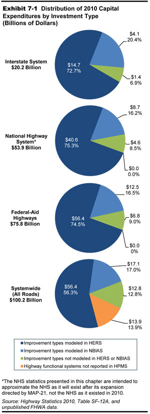
Because the HPMS sample data are available only for Federal-aid highways, the percentage of capital improvements classified as non-modeled spending is lower for Federal-aid highways than is the case systemwide. Of the $75.8 billion spent by all levels of government on capital improvements to Federal-aid highways in 2010, 74.5 percent fell within the scope of HERS, 16.5 percent fell within the scope of NBIAS, and 9.0 percent was for spending captured by neither model. The percent distribution is similar for the Interstate Highway System.
It should be noted that the statistics presented in this chapter and Chapter 8 relating to future National Highway System (NHS) investment are based on an estimate of what the NHS will look like after it is expanded pursuant to MAP-21, rather than the system as it existed in 2010. As indicated in Chapter 6, combined highway capital spending by all levels of government on the NHS in 2010 totaled $44.4 billion. The $53.9 billion NHS spending figure referenced in Exhibit 7-1 includes amounts spent on other principal arterials, as much of this mileage will be added to the NHS.
|
Treatment of the NHS in 20-Year Projections Pursuant to MAP-21, the NHS will be expanded to include additional principal arterial and connector mileage that was not part of the original system. In light of this change, projecting future NHS investment needs over 20 years based on the system as it existed in 2010 would not produce particularly useful results. Rather than dropping the NHS projections from the C&P report series until such time as the system as the formal NHS re-designation is completed, this report includes projections based on an estimate of what the system would ultimately look like, by adding in principal arterials that are not currently part of the NHS. Once the revised NHS designations have been coded into the HPMS and NBI, future editions of this report will use them for all NHS-based analyses. |
Alternative Levels of Future Capital Investment Analyzed
The HERS and NBIAS analyses presented in this chapter each assumes that capital investment within the scope of the model will grow over the 20 years at a constant annual percentage rate, which could be positive, negative, or zero. The starting point for each analysis is the level of investment in 2010, which includes one-time funding under the American Recovery and Reinvestment Act of 2009 (Recovery Act). Because future levels are measured in constant 2010 dollars, the percent rates of growth are real (inflation-adjusted). This “ramped” approach to analyzing alternative investment levels was introduced in the 2008 C&P Report. Previous editions had either assumed a fixed amount would be spent in each year or set funding levels based on benefit-cost ratios, which tended to front-load the investment within the 20-year analysis period. Chapter 9 includes an analysis of the impacts on conditions and performance of these alternative investment timing patterns, as well as an example of how the ramping approach impacts year-by-year funding levels for some of the highway investment scenarios presented in Chapter 8.
This chapter provides a quantitative picture of potential highway and bridge system outcomes under alternative assumptions about the rate of ramped investment growth. The particular investment levels identified were selected from among the results of a much larger number of model simulations. Each investment level shown corresponds to a particular target outcome, such as funding all potential capital improvements with a benefit-cost ratio above a certain threshold or attaining a certain performance standard for highways or bridges. While each of the particular rates of change selected has some specific analytical significance, the analyses presented in this chapter do not constitute complete investment scenarios, but rather form the building blocks for such scenarios, which are presented in Chapter 8.
Highway Economic Requirements System
Simulations conducted with the HERS model provide the basis for this reports analysis of investment in highway resurfacing and reconstruction as well as for highway and bridge capacity expansion. HERS employs incremental benefit-cost analysis to evaluate highway improvements based on data from the HPMS. The HPMS includes State-supplied information on current roadway characteristics, conditions, and performance and anticipated future travel growth for a nationwide sample of more than 120,000 highway sections. HERS analyzes individual sample sections only as a step toward providing results at the national level; the model does not provide definitive improvement recommendations for individual sections.
Simulations with the HERS model start by evaluating the current state of the highway system using data from the HPMS sample. These data provide information on pavements, roadway geometry, traffic volume and composition (percent trucks), and other characteristics of the sampled highway sections. For sections with one or more deficiencies identified, the model then considers potential improvements, including resurfacing, reconstruction, alignment improvements, and widening or adding travel lanes. HERS selects the improvement (or combination of improvements) with the greatest net benefits, where benefits are defined as reductions in direct highway user costs, agency costs for road maintenance, and societal costs from vehicle emissions of greenhouse gases and other pollutants. (The model uses estimates of emission costs that include damage to property and human health and, in the case of greenhouse gases, certain other potential impacts such as loss of outdoor recreation amenities.) The model allocates investment funding only to the sections where at least one of the potential improvements are projected to produce benefits exceeding construction costs.
| How closely does the HERS model simulate the actual project selection processes of State and local highway agencies? | |
|
While the HERS model is a powerful tool for projecting future investment/performance relationships, the process of project selection in the model differs from reality in several respects. HERS assumes that the allocation of total national spending on highway investment will be “economically efficient,” meaning that the projects selected will be the set that maximizes total benefits to society. The model takes no account of the division of funding authority among States and localities. For example, it could program a large increase in highway investment in a State that lacks the needed budgetary resources. The model does not attempt to simulate the influence on project selection decisions of evaluation criteria other than economic efficiency, such as perceptions of fairness and political considerations. To the extent that these other factors shape the project selection decisions, HERS may underestimate the level of investment needed to achieve a given performance or conditions target, such as maintaining average pavement ride quality.
In addition, HERS lacks access to the full array of information that governments would need to determine what is economically efficient. It relies on the HPMS database, which provides only a limited amount of information on each sampled highway section. For example, while the HPMS includes information regarding the potential for adding lanes to each highway section, and obstacles to further widening, it does not currently include information on the feasibility of alternative approaches to added capacity in a given location (construction of parallel routes, double-decking, tunneling, investments in other transportation modes, etc.). This issue is discussed further in Appendix A. |
|
HERS normally considers highway conditions and performance over a period of 20 years from the base (“current”) year, which is the most recent year for which HPMS data are available. This analysis period is split into four funding periods of equal length. After HERS performs its analysis for the first funding period, it updates the database to reflect the influences of what is predicted to happen during the first period, including the effects of the selected highway improvements. The updated database is the foundation for the analysis of conditions and performance in the second period, and so on through the fourth and last period. Appendix A contains a more detailed description of the project selection and implementation process used by HERS.
HPMS Database
The analyses presented in the 2010 C&P report relied on the 2008 HPMS database. The HPMS has subsequently been significantly modified, incorporating major changes in database structure and data items. These changes emerged from a comprehensive reassessment of how well the database was meeting user and customer needs; for details, see the HPMS Reassessment 2010+ Final Report issued in September 2008.
Changes to the HPMS
The new HPMS structure organizes data into program areas and links them together through a Geographic Information System (GIS) using spatial relationships. The revised procedures include those for creating the statistical population of highway sections from which the HPMS sample is drawn (to better ensure homogeneity over each section’s length with respect to traffic volume, number of through lanes, and other key variables) and those for averaging or summarizing measures from which different values have been estimated over a section’s length (e.g., for pavement roughness). A number of new data items have been added to the HPMS, particularly in regards to pavement characteristics and different types of pavement distresses, which are intended to support more robust analysis of pavement performance in HERS. Another key change from the HERS perspective was the replacement of an old data item regarding widening feasibility with two new items intended to provide more specific information on widening potential in terms of the specific number of lanes that could be added to a given location and obstacles to further widening; these data items are intended to support more robust analysis of widening alternatives. Appendix D discusses possible enhancements to HERS to make use of new data items on highway ramps and on measures of pavement distress other than pavement roughness.
Assessment of 2010 HPMS Sample Database’s Suitability for HERS
With the data requirements for the C&P report in mind, the initial timetable for the HPMS reassessment implementation called for States to start submitting data in the new format for the 2009 data year, in the hopes that any problems with the changeover could be addressed and resolved in time for the 2010 data submittal. However, the timetable was delayed, and only 15 States reported using the new HPMS format in 2009; for most States, 2010 was the first year in which they submitted data items under the new format.
The initial Federal Highway Administration (FHWA) data reviews conducted on the 2010 HPMS data focused on addressing issues pertaining to the types of statistics on current system characteristics and system conditions that are presented in Chapters 2 and 3. While these national-level data are considered reasonably reliable, subsequent examination of the more detailed HPMS sample data identified a large number of omissions and seemingly implausible coding for some individual items and for some combinations of data reported in different fields. Of particular concern were the large numbers of:
- Blank entries for both the International Roughness Index (IRI) and Present Serviceability Rating (PSR)
- Blank entries for pavement surface type or inconsistent entries relative to what is coded in other fields
- Miscoded responses for widening potential (at most, 20 States coded the field correctly)
- Seemingly implausible entries for the numbers of peak, counterpeak, and total lanes relative to each other
- Missing entries for single unit and combination truck traffic.
The data omissions in particular present a problem for the HERS model, which relies on having a completely populated sample data set for each individual sample record that it analyzes. In order to make use of the 2010 HPMS data, a significant effort was undertaken to impute logical values for some of the omitted data, and to develop additional screens to adjust apparent data outliers. Based on these procedures, a modified data set was then tested in HERS. This testing found anomalies in the pavement performance analysis; this was not wholly unexpected, as this was the first full national-level test of both new pavement data items and new pavement performance models that had been introduced into HERS to take advantage of these data. More puzzling were anomalies in the operational performance analysis, as these aspects of HERS had not been significantly modified, so that the changes in results could be attributed solely to the HPMS data.
In light of these issues, the FHWA has determined that for the purposes of this report, the 2008 HPMS sample data would serve as a better proxy for the “current” conditions and performance of the highway system than would the 2010 HPMS sample data set in its present form. Based on this decision, the analyses presented in this report have been developed using an older version of HERS very similar to that used for the 2010 C&P report, rather than utilizing the newer version of HERS that is customized for use with the new HPMS data format.
The FHWA will be working with the States to address issues with the HPMS sample data reporting to improve its utility for supporting future editions of the C&P report. As States become more familiar with the new HPMS data structure and data fields over time, the completeness and quality of the data should improve. To the extent that the modified HPMS structure facilitates the reporting of better data, some degree of inconsistency with the data reported in previous years can be expected.
Implications of Database Selection
Although this edition uses the same 2008 HPMS database as was used in the 2010 C&P report, other input variables were updated from 2008 to 2010, resulting in significantly different projections than those presented in the 2010 C&P report. Base-year values were updated to 2010 for prices and unit costs, average vehicle fuel efficiency, vehicle emission rates, and the level on highway investment (for runs that assume highway investment to remain at the base-year level in constant dollars). Inputs in the form of projections for fuel efficiency and vehicle emissions rates were updated to the analysis period used throughout Part II of this report, 2011-2030.
On the basis of these updates, this report considers the base year for the HERS analyses to be 2010 and the projection period to be the subsequent two decades through 2030. However, the reliance on the 2008 HPMS database should be borne in mind when interpreting the exhibits in this and following chapters. Except as noted, the base year values reported for conditions and performance indicators are actually HERS-computed values for 2008 serving as proxies for 2010 values.
Operations Strategies
Starting with the 2004 C&P report, the HERS model has considered the impacts of certain types of highway operational improvements, in which intelligent transportation systems (ITS) feature prominently. The types of strategies currently evaluated by HERS include:
- Freeway management (ramp metering, electronic roadway monitoring, variable message signs, integrated corridor management, variable speed limits, queue warning systems, lane controls)
- Incident management (incident detection, verification, and response)
- Arterial management (upgraded signal control, electronic monitoring, variable message signs)
- Traveler information (511 systems and advanced in-vehicle navigation systems with real-time traveler information).
Appendix A describes these strategies in more detail and their treatment in the HERS model. It is important to note that HERS does not subject these types of investments to benefit-cost analysis and does not directly analyze tradeoffs between them and the pavement improvements and widening options also considered by the model. Instead, operations strategies are modeled via a separate preprocessor that estimates their impact on the performance of highway sections where they are deployed. The analyses presented in this chapter assume a package of investments representing the continuation of existing deployment trends, while a sensitivity analysis presented in Chapter 10 considers the impacts of a more aggressive deployment pattern. HERS does not currently model various applications of vehicle-to-vehicle and vehicle-to-infrastructure communications that are under development because it is too early to reliably predict their impacts and patterns of deployment.
| How will Vehicle-to-Vehicle (V2V) and Vehicle-to-Infrastructure (V2I) communications potentially impact future investment needs? | |
|
Cellular, Wi-Fi, and other dedicated short-range communication technologies are expanding the possibilities for a Connected Vehicle Environment. Communications among vehicles on the road (V2V), and between these vehicles and infrastructure (V2I) hold promise for substantial reductions in crashes and vehicle emissions, and enhanced mobility through more efficient transportation systems management and operations. Adding to this potential are rapid advances in vehicle automation. For example, under advanced speed harmonization, vehicle speed would adjust automatically to speed limits that vary based on road, traffic, and weather conditions (an existing V2I application).
Additional examples of connectivity applications include blind spot monitoring/lane change warning, smart parking, forward collision warning, do-not-pass warning, curve speed warning, red light violation warning, transit pedestrian warning, cooperative adaptive cruise control, breaking assist, and dynamic lane closure management. To reach the full potential of connected vehicles will require investment, coordination, and partnership with public and private entities. As development and implementation of connected vehicle applications proceeds, additional information should make possible their representation in HERS. Research efforts by FHWA, FTA, NHTSA, AASHTO and others that will measure benefits and costs of these applications include: (1) Applications for the Environment: Real-Time Information Synthesis (AERIS) Program; (2) AASHTO Connected Vehicle Field Infrastructure Footprint Analysis; (3) Connected and Automated Vehicle Benefit Cost Analysis; and (4) Measuring Local, Regional and Statewide Economic Development Associated with the Connected Vehicle program. |
|
HERS Treatment of Traffic Growth
For each HPMS sample highway section, States provide the actual traffic volume in the base year and a forecast of traffic volume for a future year, based on available information concerning the particular section and the corridor of which it is a part. These forecasts are interpreted by HERS as having been made under the assumption that the average user cost per mile of travel, including costs of travel time, vehicle operation, and crash risk, would remain unchanged over the 20-year analysis period.
Because the present HERS analysis uses the HPMS sample data for 2008, the traffic volumes for the base and forecast years pertain to 2008 and 2028. In the 2008 database, the composite weighted average annual VMT growth rate between the 2008 base year and the forecast year is 1.85 percent. Projected VMT growth in rural areas averages 2.15 percent per year, somewhat higher than the average of 1.70 percent in urban areas.
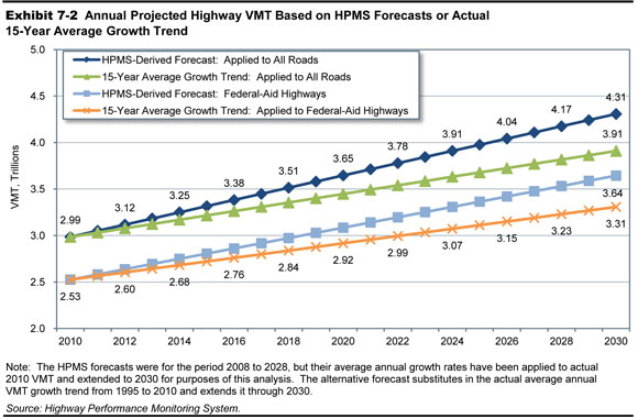
To allow for the possibility that future traffic growth will be lower than forecast in the HPMS, the HERS analysis presented in this report considers an alternative in which VMT grows at the trend rate of 1.36 percent per annum that prevailed from 1985 to 2010. In this case, the section-level forecasts of VMT from the HPMS are reduced in uniform proportion to bring the growth rate of VMT down to this level from the 1.85 percent assumed in the baseline. Exhibit 7-2 applies the alternative forecast growth rates, 1.36 percent and 1.85 percent, to actual Federal-aid highway and systemwide VMT for 2010 to derive year-by-year estimates through 2030. An underlying assumption is that VMT will grow in a linear fashion (so that 1/20th of the additional VMT is added each year), rather than geometrically (growing at a constant annual rate). With linear growth, the annual percent rate of growth gradually declines over the forecast period.
| What are some of the technical limitations associated with the analysis of alternative trend-based travel growth rates included in this section? | |
|
One of the strengths of the State-provided VMT forecasts used in the baseline analysis is their geographic specificity. Separate forecasts are provided for the more than 100,000 HPMS sample sections. The 1.85 percent average annual VMT growth rate referenced as the “forecast VMT growth” in this section reflects a compilation of these forecasts for individual sample sections.
In forming their section-specific forecasts, States can take account of specific local influences on travel growth and their own long-range planning assumptions about future travel patterns on particular routes or corridors. The inclusion of these section-level forecasts, as opposed to regional or statewide travel estimates, allows for more refined analyses of projected future investment/performance relationships. The analyses based on the alternative “trend VMT growth”, adjust the HPMS-derived forecasts for the next 20 years to match the 15-year trend from 1995 to 2010 when average VMT increased at an average annual rate of 1.36 percent. These analyses use a top-down, rather than a bottom-up approach; while they use the HPMS forecasts for individual highway sections as a starting point, these forecasts are adjusted downward in uniform proportion on a national basis. In reality, if VMT were to grow more slowly than the State projections, these differences would not be uniform, and could be heavily concentrated in particular corridors, regions, or States. Moreover, these differences could significantly impact the level of investment that might be required to achieve particular systemwide performance targets. The assumption of uniformity thus limits the reliability of this section’s analysis of the trend-based alternative VMT growth rates. |
|
Travel Demand Elasticity
One of the key features of the economic analysis in HERS is the influence of the cost of travel on the demand for travel. HERS represents this relationship as a travel demand elasticity that relates demand, measured by VMT, to average user cost per VMT. The model applies this elasticity to the forecasts of future travel (VMT) found in the HPMS sample data, which are interpreted as constant user cost forecasts. Any change that HERS projects in user cost relative to the base-year level will, through the mechanism of the travel demand elasticity, affect the model’s projection for future travel growth. For any highway investment scenario that predicts average user cost to decrease, the projected growth rate will be higher than the baseline rate derived from HPMS. The demand for travel induced by the reduction in cost could arise from various traveler responses in various ways—for example, changing route or mode of travel, or even the total amount of travel undertaken. Conversely, for scenarios in which highway user cost increases, the projected VMT growth rate will tend to be lower than the baseline rate.
HERS also allows the induced demand predicted through the elasticity mechanism to influence the cost of travel to highway users. On congested sections of highway, the initial congestion relief afforded by an increase in capacity will reduce the average user cost per VMT, which in turn will stimulate demand for travel and this increased demand will reverse a portion of the initial congestion relief. The elasticity feature operates likewise with respect to improvements in pavement quality by allowing for induced traffic that adds to pavement wear. (Conversely, an initial increase in user costs can start a causal chain with effects in the opposite direction). By capturing these offsets to initial impacts on highway user costs, HERS is able to estimate the net impacts.
Impacts of Federal-Aid Highway Investments Modeled by HERS
The present HERS analysis starts with an evaluation of the state of Federal-aid highways in the 2010 base year. Exhibit 7-1 showed that capital spending on these highways for the types of improvements modeled in HERS then amounted to $56.4 billion (out of total highway capital spending of $100.2 billion). The analysis next goes on to consider the potential impacts on system performance of raising or lowering the amount of investment within the scope of HERS at various annual rates over 20 years. Spending in any year is measured in constant 2010 dollars, so that spending and its rate of growth are both measured in real rather than nominal terms. Chapter 9 includes an illustration of how future spending levels could be converted from real to nominal dollars levels under alternative assumptions about the future inflation rate.
Selection of Investment Levels for Analysis
Exhibit 7-3 describes the significance of the 10 funding levels selected for presentation in this chapter. Some of these funding levels over the 20-year analysis period are geared toward the attainment of a specific minimum value over that period for the benefit-cost ratio (BCR). As explained in the introduction to Part II of this report, HERS ranks potential projects in order of BCR and implements them until the funding constraint is reached. The lowest BCR among the projects selected, the “marginal BCR” will vary across the four funding periods, and HERS refers to the lowest of these values across the funding periods as the “minimum BCR”. For each minimum BCR target, 1.0 or 1.5, the requisite amount of investment is determined under the alternative baseline assumptions about the future growth rate of VMT: the HPMS forecast rate (1.85 percent per annum) or the historical trend rate (1.36 percent per annum). The highest level of spending shown in Exhibit 7-3 corresponds to the annual growth rate in real spending, 3.95 percent, associated with a minimum BCR of 1.0 in the forecast VMT growth case. The attainment of this minimum BCR can be interpreted as having implemented all potentially cost-beneficial projects (BCR≥1.0). The next highest level of spending shown in Exhibit 7-3 is the estimate of what would achieve this target assuming trend-based VMT growth and averages $70.5 billion per year, which is about 18 percent less than in the forecast-based VMT growth case ($86.9 billion per year).
| HERS-Modeled Capital Investment | Minimum BCR 2 | Funding Level Description Assuming Future VMT Growth Consistent With HPMS Forecast ("Forecast") or Consistent with VMT Growth Trend "(Trend)" | ||||
|---|---|---|---|---|---|---|
| Annual Percent Change in Spending |
Average Annual Spending (Billions of 2010 Dollars) Total 1 | Assuming Forecast VMT Growth3 |
Assuming Trend VMT Growth4 | |||
| 3.95% | $86.9 | 1.00 | – | Minimum BCR=1.0 (Forecast) | ||
| 2.08% | $70.5 | 1.42 | 1.00 | Minimum BCR=1.0 (Trend) | ||
| 1.71% | $67.8 | 1.50 | 1.06 | Minimum BCR=1.5 (Forecast) | ||
| 0.72% | $60.9 | 1.73 | 1.27 | Average Delay per VMT in 2030 Matches 2010 Level (Forecast) | ||
| 0.00% | $56.4 | 1.92 | 1.42 | Constant Dollar Investment Sustained at 2010 Level | ||
| -0.32% | $54.6 | 2.01 | 1.50 | Minimum BCR=1.5 (Trend) | ||
| -0.66% | $52.7 | 2.09 | 1.58 | Average Speed in 2030 Matches 2010 Level (Forecast) | ||
| -0.95% | $51.1 | 2.17 | 1.64 | “Cost to Maintain” (Forecast) 5 | ||
| -2.62% | $43.2 | 2.64 | 2.08 | Average IRI in 2030 Matches 2010 Level (Forecast) | ||
| -4.60% | $35.7 | 2.83 | 2.53 | “Cost to Maintain” (Trend) 5 6 | ||
2 The minimum BCR represents the lowest benefit-cost ratio for any project implemented by HERS during the 20-year analysis period at the level of funding shown.
3 The “Forecast” VMT growth is computed by comparing the current average annual daily traffic (AADT) with the future AADT that are reported by the States for individual HPMS sample sections; nationally this comes out to an average annual growth rate of 1.85% . HERS assumes this represents the VMT that would occur at a constant price (i.e., highway user costs do not increase or decrease), but adjusts the growth for individual sections during its analysis in response to changes in user costs.
4 The average annual growth rate assumed in the “Trend” VMT growth analyses is 1.36%, matching the average growth rate for the 15-year period from 1995 to 2010. To implement this assumption, the future AADT values reported for each HPMS sample section in HPMS were proportionally reduced; the resulting values were assumed to be the VMT that would occur at a constant price.
5 The “Cost to Maintain” represents the average of the investment levels associated with maintaining average delay per VMT and maintaining IRI, and is used in the “Maintain Conditions and Performance” investment scenarios in Chapter 8.
6 Assuming VMT growth follows its 15-Year Trend, the annual percent change in spending at which average delay per VMT in 2030 matches the 2010 level is negative 4.61 percent, while the annual rate of spending change at which average IRI in 2030 matches the 2010 level is negative 4.60 percent. Since these values are so close, their investment levels are not identified separately, and the “Cost to Maintain” is defined around an annual change of negative 4.60 percent.
Other funding levels shown in Exhibit 7-3 are geared toward achieving a specific level of performance for a particular indicator for 2030—average congestion delay per VMT, average speed, or the average IRI. For each such indicator, the requisite amount of investment to maintain the base-year level is shown for the forecast-based VMT growth case. Shown for the cases of both forecast-based and trend-based VMT, growth is the “Cost to Maintain,” which is the average of the investment levels associated with maintaining the congestion delay and pavement roughness indicators. (Separate values are not shown for the investment levels associated with maintaining average delay per VMT and maintaining average IRI in the trend-based VMT growth case, as coincidentally they are virtually identical). In the trend-based VMT growth case, this level of investment averages $35.7 billion per year, the lowest amount shown in Exhibit 7-3, and associated rate with negative 4.3-percent annual growth in investment. (The connections between funding growth rates and performance indicators are identifiable from the exhibits presented later in this section).
The other rate of investment growth in Exhibit 7-3 is zero, for the case where average annual spending over 2010–2030 remains at the actual level of spending in 2010 in constant dollar terms.
| Why are many of the spending growth rates associated with meeting performance targets negative in this report, when they were positive in the 2010 C&P report? | |
|
Actual highway capital investment for capital improvements modeled in HERS rose from $54.7 billion in 2008 (base year for the 2010 C&P report) to $56.4 billion in 2010, a 3 percent increase in nominal dollar terms. However, this coincided with a steep drop in highway construction costs, estimated in this report to have been about 18 percent. Factoring in this price change, real spending within the scope of HERS is estimated to have increased between 2008 and 2010 by almost 26 percent. This does much to explain why the present analysis indicates that maintaining target performance indicators at their base-year levels would be consistent with spending less than in the base year, whereas the analysis presented in the 2010 C&P report indicated that spending more than in the base year would be required.
It should also be noted that 2010 highway capital investment was supplemented by one-time funding under the Recovery Act, which would make it more challenging to sustain this level of investment in the future. |
|
Investment Levels and BCRs by Funding Period
Exhibit 7-4 illustrates how the 10 alternative funding growth rates for Federal-aid highways that were selected for further analysis in this chapter would translate into cumulative spending in 5-year intervals (corresponding to 5-year analysis periods used in HERS), along with the marginal benefit-cost ratios associated with that investment. The marginal BCR is generally higher for earlier than for later subperiods, resulting in the minimum BCR over the entire analysis period, shown in the last column, equaling the marginal BCR in the last subperiod. This pattern reflects the tendency in HERS for implementing the most worthwhile improvements first. The exception to this pattern occurs when funding is assumed to decline at an annual real rate of negative 2.62 percent or more; in this case, the relative scarcity of funding toward the end of the analysis period limits what can be implemented to relatively high-return projects.
| Annual Percent Change in HERS Capital Spending | Spending Modeled in HERS (Billions of 2010 Dollars) | Marginal BCR 2 |
Minimum BCR 20-Year 2011 to 2030 | ||||||||
|---|---|---|---|---|---|---|---|---|---|---|---|
| Cumulative 5-Year 2011 to 2015 |
Cumulative 5-Year 2016 to 2020 |
Cumulative 5-Year 2021 to 2025 |
Cumulative 5-Year 2026 to 2030 |
Cumulative 5-Year 2011 to 2030 | Average Annual Spending Over 20 Years 1 | 5-Year 2011 to 2015 | 5-Year 2016 to 2020 | 5-Year 2021 to 2025 | 5-Year 2026 to 2030 | ||
| Assuming Forecast VMT Growth | |||||||||||
| 3.95% | $317 | $385 | $468 | $568 | $1,738 | $86.9 | 2.30 | 1.73 | 1.30 | 1.00 | 1.00 |
| 2.08% | $300 | $333 | $369 | $409 | $1,411 | $70.5 | 2.40 | 1.97 | 1.63 | 1.42 | 1.42 |
| 1.71% | $297 | $323 | $352 | $383 | $1,355 | $67.8 | 2.42 | 2.03 | 1.70 | 1.50 | 1.50 |
| 0.72% | $288 | $299 | $310 | $321 | $1,218 | $60.9 | 2.47 | 2.17 | 1.89 | 1.73 | 1.73 |
| 0.00% | $282 | $282 | $282 | $282 | $1,129 | $56.4 | 2.51 | 2.28 | 2.04 | 1.92 | 1.92 |
| -0.32% | $279 | $275 | $271 | $266 | $1,092 | $54.6 | 2.54 | 2.33 | 2.10 | 2.01 | 2.01 |
| -0.66% | $277 | $268 | $259 | $250 | $1,054 | $52.7 | 2.56 | 2.39 | 2.17 | 2.09 | 2.09 |
| -0.95% | $274 | $261 | $249 | $238 | $1,023 | $51.1 | 2.58 | 2.43 | 2.24 | 2.17 | 2.17 |
| -2.62% | $261 | $228 | $200 | $175 | $864 | $43.2 | 2.68 | 2.72 | 2.64 | 2.72 | 2.64 |
| -4.60% | $246 | $194 | $153 | $121 | $714 | $35.7 | 2.83 | 3.12 | 3.18 | 3.38 | 2.83 |
| Assuming Trend VMT Growth | |||||||||||
| 2.08% | $300 | $333 | $369 | $409 | $1,411 | $70.5 | 2.18 | 1.66 | 1.22 | 1.00 | 1.00 |
| 1.71% | $297 | $323 | $352 | $383 | $1,355 | $67.8 | 2.20 | 1.71 | 1.28 | 1.06 | 1.06 |
| 0.72% | $288 | $299 | $310 | $321 | $1,218 | $60.9 | 2.27 | 1.84 | 1.44 | 1.27 | 1.27 |
| 0.00% | $282 | $282 | $282 | $282 | $1,129 | $56.4 | 2.32 | 1.93 | 1.57 | 1.42 | 1.42 |
| -0.32% | $279 | $275 | $271 | $266 | $1,092 | $54.6 | 2.34 | 1.98 | 1.64 | 1.50 | 1.50 |
| -0.66% | $277 | $268 | $259 | $250 | $1,054 | $52.7 | 2.36 | 2.03 | 1.70 | 1.58 | 1.58 |
| -0.95% | $274 | $261 | $249 | $238 | $1,023 | $51.1 | 2.38 | 2.07 | 1.75 | 1.64 | 1.64 |
| -2.62% | $261 | $228 | $200 | $175 | $864 | $43.2 | 2.49 | 2.33 | 2.10 | 2.08 | 2.08 |
| -4.60% | $246 | $194 | $153 | $121 | $714 | $35.7 | 2.62 | 2.67 | 2.53 | 2.63 | 2.53 |
2 The marginal BCR represents the lowest benefit-cost ratio for any project implemented during the period identified at the level of funding shown. The minimum BCRs, indicated by bold font and also shown in the last column, are the smallest of the marginal BCRs across the funding periods.
As shown in Exhibit 7-4, achieving a minimum BCR of 1.0 is estimated to require $1.738 trillion over the analysis period when forecast VMT growth is assumed and about $1.411 trillion when trend VMT growth is assumed. Applying the more restrictive minimum BCR target of 1.50 would require, respectively, 15 percent and 20 percent less than these amounts ($1.355 trillion and $1.092 trillion over the analysis period).
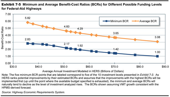
Further evident in Exhibits 7-3 and 7-4 is the inverse relationship described in the introduction to Part II between the minimum BCR and the level of investment. Exhibit 7-5 graphs this inverse relationship, as well as that between the average BCR and the level of investment. At any given level of average annual investment, the average BCR always exceeds the marginal BCR. For example, at the lowest level of investment considered, $714 billion over 20 years, the average BCR of 5.82 exceeds the minimum BCR of 2.83, assume forecast VMT growth.
Impact of Future Investment on Highway Pavement Ride Quality
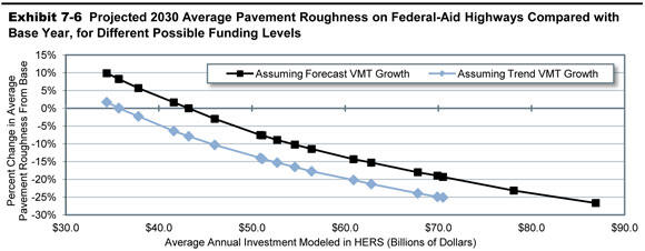
The primary measure in HPMS of highway physical condition is pavement ride quality as measured by the IRI index of pavement roughness (defined in Chapter 3). The HERS analysis presented in this report focuses on VMT-weighted IRI values; the average IRI values shown thus reflect the pavement ride quality experienced on a typical mile of travel. Exhibit 7-6 shows how the projection for the average IRI on Federal-aid highways in 2030 varies with the total amount of HERS-modeled investment and between the assumptions regarding VMT growth. Also shown is the portion of investment that HERS allocates to system rehabilitation, which is more significant than investment in system expansion in influencing average pavement ride quality.
| HERS-Modeled Capital Investment | Projected Impacts on Federal-Aid Highways 3 Average IRI (VMT-Weighted) | |||||||
|---|---|---|---|---|---|---|---|---|
| Annual Percent Change in Spending |
Average Annual Spending (Billions of 2010 Dollars) Total 1 | Average Annual Spending (Billions of 2010 Dollars) System Rehabilitation 2 If Forecast VMT Growth |
Average Annual Spending (Billions of 2010 Dollars) System Rehabilitation 2 |
Projected 2030 Level If Forecast VMT Growth |
Projected 2030 Level If Trend VMT Growth | Percent Change Relative to Base Year If Forecast VMT Growth | Percent Change Relative to Base Year If Trend VMT Growth |
|
| 3.95% | $86.9 | $43.9 | – | 83.9 | – | -26.7% | – | |
| 2.08% | $70.5 | $36.7 | $40.6 | 92.3 | 85.7 | -19.3% | -25.1% | |
| 1.71% | $67.8 | $35.6 | $39.3 | 93.8 | 87.0 | -18.0% | -24.0% | |
| 0.72% | $60.9 | $32.6 | $35.8 | 98.0 | 91.3 | -14.3% | -20.2% | |
| 0.00% | $56.4 | $30.6 | $33.6 | 101.3 | 94.1 | -11.5% | -17.7% | |
| -0.32% | $54.6 | $29.7 | $32.6 | 102.7 | 95.5 | -10.2% | -16.5% | |
| -0.66% | $52.7 | $28.9 | $31.6 | 104.2 | 96.9 | -8.9% | -15.3% | |
| -0.95% | $51.1 | $28.1 | $30.8 | 105.7 | 98.1 | -7.6% | -14.2% | |
| -2.62% | $43.2 | $24.2 | $26.6 | 114.4 | 105.4 | 0.0% | -7.9% | |
| -4.60% | $35.7 | $20.6 | $22.6 | 123.8 | 114.4 | 8.2% | 0.0% | |
| Base Year Value: | 114.4 | |||||||
2 The amounts shown represent the portion of HERS-modeled spending directed toward system rehabilitation, rather than system expansion, which is influenced by the assumption made about future VMT growth rates.
3 The HERS model relies on information from the HPMS sample section database, which is limited to those portions of the road network that are generally eligible for Federal funding (i.e., “Federal-aid highways”) and excludes roads classified as rural minor collectors, rural local, and urban local.
For each of the funding levels analyzed, HERS would direct a greater share of total spending toward system rehabilitation assuming the trend rate of VMT growth (1.36 percent per annum) rather than the forecast rate of VMT growth (1.85 percent per annum). The lower VMT under the trend growth case also results in less pavement damage from traffic. Consequently, for any given level of investment in Federal-aid highways, Exhibit 7-6 indicates the average IRI projected for 2030 to be lower in the trend than in the forecast case. For example, assuming that real investment in highways remains at the 2010 base year level of $56.4 billion, the projection is for the average IRI to decline by 17.7 percent to 94.1 in the trend VMT growth case, while it would only decline by 11.5 percent to 101.3 for the forecast VMT growth case.
For almost all combinations of investment level and traffic growth that Exhibit 7-6 presents, pavements on Federal-aid highways are projected to be smoother on average in 2030 than in 2010. The exception combines spending declining at an average annual rate of 4.6 percent with traffic growing at the forecast rate (1.85 percent per annum). For those circumstances, HERS projects an 8.2-percent increase in average pavement roughness. The same rate of decline in spending combined with the trend rate of traffic growth (1.36 percent per annum) is projected to maintain the average IRI at the base year level. The rate of spending growth that would maintain average IRI at the 2010 level case is higher when traffic is assumed to grow at the forecast rate, but still negative (-2.62 percent per annum).
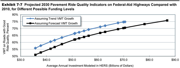
Exhibit 7-7 shows the HERS projections for the percentage of travel occurring on pavements with ride quality that would be rated good or acceptable based on the IRI thresholds set in Chapter 3. Under all circumstances represented in the exhibit, the 2030 projection for the percent of travel occurring on pavements with good ride quality exceeds the 50.6 percent that occurred in 2010. With traffic assumed to grow at the forecast rate, the projection for 2030 ranges from 75.8 percent at the highest level of investment modeled, which implements all projects with BCR≥1.0, to 51.0 percent at the lowest level, which would reduce investment at an average annual rate of 4.6 percent. When zero change from the 2010 level of investment is modeled, the projections for 2030 in the forecast growth case are for pavements with good ride quality to carry 64.7 percent of travel. In the trend traffic case, the corresponding projections are 4 to 5 percentage points higher, reflecting the greater share of investment directed toward system rehabilitation.
| HERS-Modeled Capital Investment | Projected Impacts on Federal-Aid Highways | ||||||
|---|---|---|---|---|---|---|---|
| Annual Percent Change in Spending | Average Annual Spending (Billions of 2010 Dollars) Total | Average Annual Spending (Billions of 2010 Dollars) System Rehabilitation If Forecast VMT Growth | Average Annual Spending (Billions of 2010 Dollars) System Rehabilitation If Trend VMT Growth |
Percent of 2030 VMT on Roads With IRI<95 (Good Ride Quality)1 If Forecast VMT Growth |
Percent of 2030 VMT on Roads With IRI<95 (Good Ride Quality)1 If Trend VMT Growth |
Percent of 2030 VMT on Roads With IRI<170 (Acceptable Ride Quality)1 If Forecast VMT Growth | Percent of 2030 VMT on Roads With IRI<170 (Acceptable Ride Quality)1 If Trend VMT Growth |
| 3.95% | $86.9 | $43.9 | – | 75.8% | – | 93.4% | – |
| 2.08% | $70.5 | $36.7 | $40.6 | 70.5% | 74.8% | 90.8% | 93.1% |
| 1.71% | $67.8 | $35.6 | $39.3 | 69.5% | 74.0% | 90.4% | 92.6% |
| 0.72% | $60.9 | $32.6 | $35.8 | 66.8% | 71.2% | 89.1% | 91.3% |
| 0.00% | $56.4 | $30.6 | $33.6 | 64.7% | 69.2% | 88.1% | 90.3% |
| -0.32% | $54.6 | $29.7 | $32.6 | 63.9% | 68.3% | 87.6% | 89.9% |
| -0.66% | $52.7 | $28.9 | $31.6 | 62.9% | 67.3% | 87.2% | 89.5% |
| -0.95% | $51.1 | $28.1 | $30.8 | 62.1% | 66.5% | 86.7% | 89.1% |
| -2.62% | $43.2 | $24.2 | $26.6 | 56.6% | 61.6% | 84.0% | 86.8% |
| -4.60% | $35.7 | $20.6 | $22.6 | 51.0% | 55.8% | 81.5% | 84.0% |
| Base Year Values 2: | 50.6% | 82.0% | |||||
2 Base Year values shown are 2010 values reported in Chapter 3, rather than those reflected in the 2008 HPMS sample dataset.
In almost all the circumstances considered, Exhibit 7-7 also shows increases relative to the base year level of 82.0 percent in the proportion of travel occurring on pavements with ride quality rated as acceptable. With traffic assumed to grow at the forecast rate, the projection for 2030 ranges from 93.4 percent at the highest level of investment modeled to 81.5 percent at the lowest. When no change from the 2010 level of investment is modeled, 88.1 percent of travel in 2030 in the forecast traffic growth case is projected to occur on pavements with acceptable ride quality. In the trend traffic growth case, the corresponding projections are 2 to 3 percentage points higher. As noted in Chapter 3, the IRI threshold of 170 used to identify acceptable ride quality was originally set to measure performance on the NHS and may not be fully applicable to non-NHS routes, which tend to have lower travel volumes and speeds.
Impact of Future Investment on Highway Operational Performance
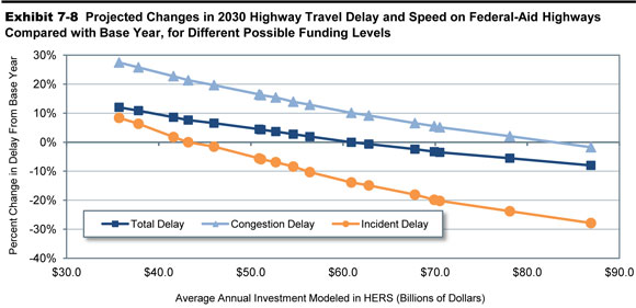
Exhibit 7-8 shows the HERS projections for travel time-related indicators of highway performance for the case where traffic grows as forecast in the HPMS. As noted above, HERS assumes the continuation of existing trends in the deployment of certain system management and operations strategies. Among these strategies are several, such as freeway incident management programs, that can be expected to mitigate delay associated with isolated incidents more than the delay associated with recurring congestion (“congestion delay”). In line with this, Exhibit 7-8 shows the amount of incident delay decreasing relative to congestion delay over the period 2010-2030. Assuming that investment within the scope of HERS remains in real terms at its 2010 level, the model projects incident delay per VMT on Federal-aid highways to decrease 10.3 percent between 2010 and 2030, and congestion delay to increase 12.9 percent.
| HERS-Modeled Capital Investment | Projected Impacts on Federal-Aid Highways1 | ||||||
|---|---|---|---|---|---|---|---|
| Annual Percent Change in Spending | Average Annual Spending (Billions of 2010 Dollars) Total2 |
Average Annual Spending (Billions of 2010 Dollars) System Expansion3 |
Annual Hours of Delay per Vehicle4 |
Percent Change Relative to Baseline Total Delay per VMT |
Percent Change Relative to Baseline Congestion Delay per VMT |
Percent Change Relative to Baseline Incident Delay per VMT | Average Speed in 2030 (mph) |
| 3.95% | $86.9 | $43.0 | 47.3 | -8.0% | -1.7% | -27.9% | 44.3 |
| 2.08% | $70.5 | $33.9 | 49.6 | -3.5% | 5.2% | -20.2% | 43.8 |
| 1.71% | $67.8 | $32.2 | 50.2 | -2.4% | 6.6% | -18.1% | 43.7 |
| 0.72% | $60.9 | $28.3 | 51.4 | 0.0% | 10.1% | -13.9% | 43.5 |
| 0.00% | $56.4 | $25.9 | 52.4 | 1.9% | 12.9% | -10.3% | 43.3 |
| -0.32% | $54.6 | $24.9 | 52.8 | 2.8% | 14.0% | -8.4% | 43.3 |
| -0.66% | $52.7 | $23.8 | 53.3 | 3.7% | 15.4% | -6.9% | 43.2 |
| -0.95% | $51.1 | $23.0 | 53.6 | 4.3% | 16.2% | -5.9% | 43.1 |
| -2.62% | $43.2 | $19.0 | 55.3 | 7.6% | 21.4% | 0.0% | 42.8 |
| -4.60% | $35.7 | $15.1 | 57.6 | 12.0% | 27.5% | 8.4% | 42.3 |
| Base Year Values: | 51.4 | 43.2 | |||||
2 The amounts shown represent the average annual investment over 20 years by all levels of government combined that would occur if such spending grows annually in constant dollar terms by the percentage shown in each row of the first column.
3 The amounts shown represent the portion of HERS-modeled spending directed toward system expansion, rather than system rehabilitation, which is influenced by the assumption made about future VMT growth rates.
4 The values shown were computed by multiplying HERS estimates of average delay per VMT by 11,853, the average VMT per registered vehicle in 2010. HERS does not forecast changes in VMT per vehicle over time. The HERS delay figures include delay attributable to stop signs and signals, as well as delay resulting from congestion and incidents.
The results in Exhibit 7-8 also reveal investment within the scope of HERS to be a potent instrument for reducing congestion delay. Exhibit 7-8 splits out the portion of that investment that HERS programs for system expansion (such as the widening of existing highways or building new routes in existing corridors), which will tend to reduce congestion delay more than spending on system rehabilitation.
When average annual total investment is assumed to be sustained at the 2010 level of $56.4 billion, total delay per VMT in 2030 is projected to be 1.9 percent higher than in 2010. If instead annual total investment is assumed to average the $86.9 billion that HERS estimates would be needed to fund all improvements with BCR≥1.0, the projected change in total delay per VMT is a reduction of 8.0 percent from the 2010 level. For annual congestion delay per vehicle in 2030, the projections indicate that the effect of this difference in investment levels is to save 5.1 hours (47.1 hours assuming $86.9 billion per year versus 52.4 hours at actual 2010 spending). In contrast, at assumed investment levels much lower than what was spent in 2010, the projections are for significant increases in congestion delay per VMT—12.0 percent at the lowest level of investment considered, an annual average of $35.7 billion.
| How large is the investment backlog estimated by HERS? | |
|
The investment backlog represents all improvements that could be economically justified for immediate implementation, based solely on the current conditions and operational performance of the highway system (without regard to potential future increases in VMT or potential future physical deterioration of pavements).
The HERS model does not routinely produce rolling backlog figures over time as an output, but is equipped to do special analyses to identify the base year backlog. To determine which action items to include in the backlog, HERS evaluates the current state of each highway section before projecting the effects of future travel growth on congestion and pavement deterioration. Any potential improvement that would correct an existing pavement or capacity deficiency and that has a BCR greater than or equal to 1.0 is considered part of the current highway investment backlog. HERS estimates the size of the backlog as $486.6 billion for Federal-aid highways, stated in constant 2010 dollars. The estimated backlog for the Interstate System is $145.9 billion; adding in other principal arterials produces an estimated backlog of $344.8 billion for the expanded NHS. The investment levels associated with a minimum BCR of 1.0 presented in this chapter would fully eliminate this backlog, as well as addressing other deficiencies that arise over the next 20 years, when it is cost beneficial to do so. It should be noted that these figures reflect only a subset of the total highway investment backlog; they do not include the types of capital improvements modeled in NBIAS (presented later in this chapter) or the types of capital improvements not currently modeled in HERS or NBIAS. Chapter 8 presents an estimate of the combined backlog for all types of improvements. |
|
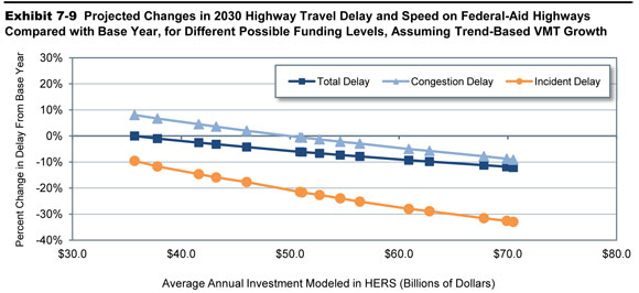
Exhibit 7-9 presents results from HERS simulations in which the baseline VMT growth conforms to 15-year historical trend rather than the HPMS forecasts. Because this reduces the rate of VMT growth, the projections of delay for 2030 are lower than in Exhibit 7-8. For the case where spending continues at the 2010 level, annual delay per vehicle is projected at 47.4 hours versus the 52.4 hours that was projected in Exhibit 7-8 when forecast traffic growth was assumed. The impacts on delay of varying the level of investment are somewhat smaller, as well. For example, increasing average annual investment from the 2010 level to $68.4 billion reduces the 2030 projection of annual delay per vehicle by 1.8 hours (from 47.4 to 45.6), whereas the corresponding reduction in Exhibit 7-8 was 2.2 hours.
| HERS-Modeled Capital Investment | Projected Impacts on Federal-Aid Highways1 | ||||||
|---|---|---|---|---|---|---|---|
| Annual Percent Change in Spending | Average Annual Spending (Billions of 2010 Dollars) Total2 |
Average Annual Spending (Billions of 2010 Dollars) System Expansion 3 |
Annual Hours of Delay per Vehicle 4 |
Percent Change Relative to Baseline Total Delay per VMT |
Percent Change Relative to Baseline Congestion Delay per VMT |
Percent Change Relative to Baseline Incident Delay per VMT | Average Speed in 2030 (mph) |
| 2.08% | $70.5 | $30.0 | 45.2 | -12.1% | -9.1% | -33.0% | 44.6 |
| 1.71% | $67.8 | $28.5 | 45.6 | -11.2% | -7.8% | -31.6% | 44.5 |
| 0.72% | $60.9 | $25.1 | 46.6 | -9.3% | -5.0% | -28.0% | 44.3 |
| 0.00% | $56.4 | $22.8 | 47.4 | -7.8% | -2.9% | -25.2% | 44.2 |
| -0.32% | $54.6 | $22.0 | 47.6 | -7.3% | -2.2% | -23.9% | 44.2 |
| -0.66% | $52.7 | $21.1 | 48.0 | -6.7% | -1.3% | -22.6% | 44.1 |
| -0.95% | $51.1 | $20.3 | 48.2 | -6.2% | -0.7% | -21.6% | 44.0 |
| -2.62% | $43.2 | $16.6 | 49.7 | -3.2% | 3.6% | -15.9% | 43.8 |
| -4.60% | $35.7 | $13.1 | 51.4 | 0.0% | 8.0% | -9.5% | 43.4 |
| Base Year Values: | 51.4 | 43.2 | |||||
2 The amounts shown represent the average annual investment over 20 years by all levels of government combined that would occur if such spending grows annually in constant dollar terms by the percentage shown in each row of the first column.
3 The amounts shown represent the portion of HERS-modeled spending directed toward system expansion, rather than system rehabilitation, which is influenced by the assumption made about future VMT growth rates.
4 The values shown were computed by multiplying HERS estimates of average delay per VMT by 11,853, the average VMT per registered vehicle in 2010. HERS does not forecast changes in VMT per vehicle over time. The HERS delay figures include delay attributable to stop signs and signals, as well as delay resulting from congestion and incidents.
Whichever the traffic growth assumption, forecast or trend, it is important to bear in mind some traffic basics when interpreting these results. In addition to congestion and incident delay, some delay inevitably results from traffic control devices. For this reason, and because traffic congestion occurs only at certain places and times, Exhibits 7-8 and 7-9 show the variation in the level of investment as having less of an impact on projections for total delay and average speed than on the projections for congestion and incident delay. In addition, while the impacts of additional investment on average speed are proportionally small—when trend traffic growth is assumed, investing enough to implement all cost beneficial projects rather than at the 2010 level increases average speed projected for 2030 from 44.2 mph to 44.6 mph—these impacts apply to a vast amount of travel, so that the associated savings in user cost are not necessarily small relative to the cost of the investment.
Impact of Future Investment on Highway User Costs
In the HERS model, the benefits from highway improvements are the reductions in highway user costs, agency costs, and societal costs of vehicle emissions. In measuring the highway user costs, the model includes the costs of travel time, vehicle operation, and crashes, but excludes from vehicle operating costs taxes imposed on highway users (such as motor fuel taxes and vehicle registration fees). As discussed in the Introduction to Part II, the exclusion of these taxes conforms with the principle in benefit-cost analysis of measuring the costs of transportation inputs as their opportunity cost to society. The exclusion also makes the measure of user costs more of an indicator of highway conditions and performance, of which the amount paid in highway-user taxes provides no indication.
Impact on Overall User Cost
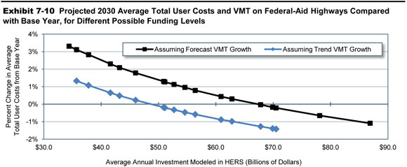
For Federal-aid highways, HERS estimates that user costs—the costs of travel time, vehicle operation, and crashes—averaged $1.030 per mile of travel in the base year (Exhibit 7-10). When baseline traffic is assumed to grow as forecast, the average user cost is generally higher in the 2030 projection than in the base year estimate. Average user cost is projected to increase between 2010 and 2030 by 0.8 percent and by 2.1 percent under the assumptions that real annual spending remains at the base year level or, alternatively, decreases annually at the rate geared toward maintaining average pavement roughness (2.62 percent). Decreases in average user cost are projected for the two highest levels of spending considered. At the level HERS indicates would be needed to fund all cost-beneficial projects (averaging $86.9 billion annually), average user cost per mile of travel in 2030 is projected to be $1.018, or 1.1 percent less than in the base year. Exhibit 7-10 also reveals that assuming baseline traffic growth to follow trend rather than the HPMS forecasts reduces the projections of average user cost at a given level of investment by 1 to 2 percent.
| HERS-Modeled Capital Investment | Projected Impacts on Federal-Aid Highways* | ||||||
|---|---|---|---|---|---|---|---|
| Annual Percent Change in Spending |
Average Annual Spending (Billions of 2010 Dollars) |
Average Total User Costs ($/VMT) If Forecast VMT Growth |
Average Total User Costs ($/VMT) If Trend VMT Growth |
Percent Change in User Costs per VMT, Relative to Base Year If Forecast VMT Growth |
Percent Change in User Costs per VMT, Relative to Base Year If Trend VMT Growth |
Projected 2030 VMT on Federal-aid Highways (Trillions of VMT)* If Forecast VMT Growth |
Projected 2030 VMT on Federal-aid Highways (Trillions of VMT)* If Trend VMT Growth |
| 3.95% | $86.9 | $1.018 | – | -1.1% | – | 3.629 | – |
| 2.08% | $70.5 | $1.027 | $1.015 | -0.2% | -1.4% | 3.612 | 3.303 |
| 1.71% | $67.8 | $1.029 | $1.017 | 0.0% | -1.3% | 3.608 | 3.300 |
| 0.72% | $60.9 | $1.034 | $1.021 | 0.4% | -0.9% | 3.599 | 3.293 |
| 0.00% | $56.4 | $1.038 | $1.024 | 0.8% | -0.6% | 3.592 | 3.287 |
| -0.32% | $54.6 | $1.040 | $1.025 | 1.0% | -0.5% | 3.589 | 3.285 |
| -0.66% | $52.7 | $1.041 | $1.026 | 1.1% | -0.3% | 3.586 | 3.282 |
| -0.95% | $51.1 | $1.043 | $1.028 | 1.3% | -0.2% | 3.584 | 3.280 |
| -2.62% | $43.2 | $1.051 | $1.035 | 2.1% | 0.5% | 3.568 | 3.268 |
| -4.60% | $35.7 | $1.062 | $1.043 | 3.1% | 1.3% | 3.550 | 3.253 |
| Base Year Values: | $1.030 | 2.520 | |||||
| How much does HERS modify the baseline projections of VMT? | |
|
The modification is largest at the lowest investment level presented in Exhibit 7-10, which averages $35.7 billion per year and corresponds to negative 4.6 percent annual growth in spending. At this investment level, average user costs are projected to increase between 2010 and 2030 by 3.1 percent when the baseline traffic growth is assumed to be as forecast in HPMS. The projected increase in average user cost operates through the HERS elasticity mechanism to reduce the VMT projection for 2030. The increase from 2.520 trillion VMT in the base year to 3.550 trillion VMT in 2030 translates into an average annual VMT growth rate of 1.73 percent, which falls below the 1.85 percent growth rate forecast in HPMS.
Similarly, when traffic growth is assumed to follow the 15-year trend, average user costs per VMT are projected to increase by 1.3 percent; the increase from 2.520 trillion VMT to 3.253 trillion VMT translates into an average annual VMT growth rate of 1.28 percent, rather than the 1.36 percent annual growth rate assumed if user costs remained constant. In the present analysis, the percent changes in average user cost are relatively small. For this reason, and because HERS incorporates the indications from available evidence that travel demand is not highly sensitive to price, HERS only slightly modifies the baseline projection of VMT. |
|
The projections in Exhibit 7-10 for VMT on Federal-aid highways incorporate the effects on travel demand of changes in average user cost. These outputs from the HERS analysis differ from the “trend” and “forecast” projections of VMT on Federal-aid highways that are inputs to the analysis. The input projections, which were shown in Exhibit 7-2, are interpreted as representing the baseline levels of traffic in the absence of any change in average user cost from the 2010 level. The 2030 traffic levels presented in Exhibit 7-10 are thus higher or lower than these baseline levels according to whether average user cost is projected to decrease or increase.
Impact on User Cost Components
Exhibit 7-11 shows the projected changes from 2010 to 2030 in average user cost of travel on Federal-aid highways by cost component. The cost of crashes is the component least sensitive to the assumed level of highway investment, which as an annual average varies between $35.7 billion and $86.9 billion or $70.5 billion depending on whether baseline VMT growth is assumed to follow the HPMS forecast or the 15-year trend. Compared with the lowest level, the highest level of spending reduces the crash cost per VMT by 0.7 percent (forecast case) or 0.1 percent (trend case). These levels of spending are limited to the types of improvements that HERS evaluates, which are basically system rehabilitation and expansion. Because the HPMS lacks detailed information on the current location and characteristics of safety-related features (e.g., guardrail, rumble strips, roundabouts, yellow change intervals at signals), safety-focused investments are not evaluated. Thus, the findings presented in Exhibit 7-11 establish nothing about how such investments affect highway safety.
| HERS-Modeled Capital Investment | Projected Impacts on Federal-Aid Highways Percent Change in User Costs per VMT in 2030, Relative to Base Year | ||||||
|---|---|---|---|---|---|---|---|
| Annual Percent Change in Spending |
Average Annual Spending (Billions of 2010 Dollars) |
Travel Time Costs If Forecast VMT Growth |
Travel Time Costs If Trend VMT Growth |
Vehicle Operating Costs1 If Forecast VMT Growth |
Vehicle Operating Costs 1 If Trend VMT Growth |
Crash Costs 2 If Forecast VMT Growth |
Crash Costs 2 If Trend VMT Growth |
| 3.95% | $86.9 | -3.0% | – | 0.2% | – | 1.1% | – |
| 2.08% | $70.5 | -1.8% | -3.9% | 1.0% | 0.8% | 1.3% | 0.1% |
| 1.71% | $67.8 | -1.6% | -3.7% | 1.1% | 0.9% | 1.3% | 0.1% |
| 0.72% | $60.9 | -0.9% | -3.2% | 1.6% | 1.3% | 1.4% | 0.2% |
| 0.00% | $56.4 | -0.4% | -2.8% | 1.8% | 1.5% | 1.5% | 0.3% |
| -0.32% | $54.6 | -0.2% | -2.7% | 2.0% | 1.7% | 1.5% | 0.3% |
| -0.66% | $52.7 | 0.1% | -2.5% | 2.1% | 1.8% | 1.5% | 0.4% |
| -0.95% | $51.1 | 0.2% | -2.4% | 2.3% | 1.9% | 1.6% | 0.4% |
| -2.62% | $43.2 | 1.2% | -1.5% | 3.2% | 2.7% | 1.6% | 0.4% |
| -4.60% | $35.7 | 2.5% | -0.6% | 4.1% | 3.7% | 1.8% | 0.6% |
2 The HPMS does not contain the type of detail that would be needed to conduct an analysis of targeted safety enhancements. The crash costs estimated by the HERS model represent ancillary impacts associated with pavement and capacity improvements and are heavily influenced by traffic volume and speed.
Crash costs also form the smallest of the three components of highway user costs. For 2010 travel on Federal-aid highways, HERS estimates the breakdown by cost component to be crash cost, 13.6 percent; travel time cost, 44.9 percent, and vehicle operating cost, 41.5 percent. Research under way to update the vehicle operating cost equations in HERS (see Appendix D) may somewhat alter the split among these costs, but crash costs will remain a small component. Although highway trips always consume traveler time and resources for vehicle operation, only a small fraction involve crashes. In addition, most crashes are non-catastrophic: particularly on urban highways, many involve only damage to property without anyone being injured.
The projections for the travel time costs are somewhat more sensitive to the assumed level of investment than are the projections for vehicle operating costs. When baseline VMT growth is based on HPMS forecasts, the projected 2010-2030 change in travel cost per VMT ranges from a decrease of 3.5 percent at the highest level of assumed investment to an increase of 2.5 percent at the lowest. This implies that investing at the highest rather than the lowest level would reduce the per VMT cost of travel in 2030 by 5.4 percent (= (035+.025)/(1-.025)). For vehicle operating cost, the corresponding estimate is a reduction of 3.3 percent. When VMT growth is based on trend rather than forecasts, the projections of travel time and vehicle operating cost are lower and less sensitive to variation in the assumed investment level. Investing at the highest level shown for the trend forecast case rather than at the lowest level reduces the projected time cost of travel in 2030 by 3.7 percent and the projected vehicle operating cost by 2.8 percent.
For vehicle operating costs per VMT, all the projections in Exhibit 7-11 show levels in 2030 to exceed those for 2010. This uniformity contrasts with the mixed pattern in the projections for travel time cost and reflects the assumption of future increases in motor fuel prices. For these prices and for vehicle fuel economy, the assumptions are based on projections from the Energy Information Administration (EIA) Annual Energy Outlook 2012. The weighted average price of gasoline and diesel fuel is assumed to increase between 2010 and 2030 by 45 percent more than the consumer price index. This increase outweighs the fuel cost savings that would result from the improvements in vehicle energy efficiency that the EIA projects for this same period; these equate to increases in average MPG of 32.8 percent for light-duty vehicles, 30.0 percent for two-axle trucks, and 19.4 percent for 3+ axle trucks. These projections incorporate the effect of increases in Corporate Average Fuel Economy (CAFE) standards and U.S. Environmental Protection Agency (EPA) standards for emissions of greenhouse gases by automobiles and light trucks through model year 2016, as well as new standards for fuel efficiency and greenhouse gas emissions for medium- and heavy-duty trucks through model year 2018 adopted by U.S. Department of Transportation (DOT) and EPA.
| What changes in CAFE standards have recently been adopted, and what impacts are these changes expected to have? | |
|
On May 7, 2010, NHTSA and EPA jointly adopted Corporate Average Fuel Economy (CAFE) and carbon dioxide (CO2) emission standards for cars and light trucks produced during model years 2012 through 2016. In combination with NHTSA’s previous actions, this rule raised required fuel economy levels for cars from 27.5 miles per gallon (mpg) in model year 2010 to 37.8 mpg for model year 2016, and those for light trucks from 23.5 mpg in 2010 to 28.8 mpg for 2016. On August 28, 2012, the two agencies adopted new rules that further increased CAFE standards for model year 2021 to 46.1 to 46.8 mpg for automobiles and to 32.6 to 33.3 mpg for light trucks; this most recent action also established tentative CAFE standards for model year 2025 of 55.3 to 56.2 mpg for cars and 39.3 to 40.3 mpg for light trucks.
The impacts of these standards on the fuel economy of the overall vehicle fleet will continue to grow for many years beyond 2025, as new vehicles meeting the higher fuel economy requirements gradually replace older, less-fuel-efficient vehicles. In announcing the most recent increases in CAFE standards, NHTSA estimated that the cumulative effects of its actions would be to save more than 500 billion gallons of fuel and reduce carbon dioxide emissions by 6 billion metric tons over the lifetimes of cars and light trucks produced in 2011 through 2025. The agency also estimated that its standards would save the Nation’s drivers more than $1.7 trillion in fuel costs over these vehicles’ lifetimes. In 2011, NHTSA and EPA also established new fuel efficiency and CO2 emission standards for medium- and heavy-duty trucks produced from 2014 through 2018. These standards are expected to reduce fuel consumption by an additional 22 billion gallons, while further reducing CO2 emissions by nearly 270 million metric tons. |
|
Impacts of NHS Investments Modeled by HERS
As described in Chapter 2, the NHS includes the Interstate System as well as other routes most critical to national defense, mobility, and commerce. As noted earlier, the NHS analyses presented in this chapter are based on an estimate of what the NHS will look like after it is expanded pursuant to MAP-21, rather than the actual system as it existed in 2010.
This section examines the total spending modeled in HERS, identifying the portion of this investment that is directed by the model to the NHS, and the impacts that such investment could have on future NHS conditions and performance. For Federal-aid highways, the preceding analysis in this chapter examined the effect on the HERS projections of replacing the HPMS traffic forecasts with trend traffic growth. In analyzing investments in the NHS portion of Federal-aid highways, this section assumes traffic growth as forecast in the HPMS.
HERS allocates a portion of future investment in Federal-aid highways to the NHS based on the model’s engineering and economic criteria, which give funding priority to high-BCR projects. The levels of future investment in Federal-aid highways considered in this section’s analysis are either identical to or counterparts of levels considered in this chapter’s preceding sections. Carried over from the preceding analysis are the investment levels tied to a specific minimum BCR among all improvements to the Federal-aid highways that HERS programs over the analysis period. Also included are levels of investment in Federal-aid highways tied to one of the goals considered in the preceding analysis, such as maintaining average pavement roughness at the base year level, except that the goals are now limited to the NHS. In the simulations with these investment levels, HERS allocates to the NHS the amount needed to achieve the goal for the NHS without regard to whether or not the same goal is met for other Federal-aid highways.
| How were the seven NHS investment levels presented in Exhibits 7-12 and 7-13 selected? | |
|
As MAP-21 directs that the NHS be expanded, the 20-year NHS projections presented in this report were based on all sections coded in HPMS as being on the NHS, plus those other principal arterials that are not currently part of the NHS. While this will not exactly match the scope of the NHS in the future (some sections currently coded as principal arterials may not be ultimately be included in the NHS, and some additional connector mileage may be included), it represents a reasonably close approximation for purposes of the types of analyses presented.
The investment levels associated with minimum BCR cutoffs of 1.00 and 1.50 were derived from the same HERS runs identified in Exhibit 7-3 as associated with these cutoffs assuming VMT growth consistent with the HPMS-derived forecast. The investment levels shown reflect the portion of spending in those runs that was directed to the NHS. The remaining five levels were selected using comparable criteria to those identified in Exhibit 7-3, but in terms of the NHS in particular, rather than Federal-aid highways in general. The 20-year investment level associated with a minimum BCR cutoff of 1.78 results in an average annual investment level of $40.6 billion, consistent with spending on the NHS in 2010 on types of capital improvements modeled in HERS. The investment level associated with a minimum BCR cutoff of 2.49 was selected to be included because it results in projected average speed in 2030 matching the base year level. Investing at the level associated with a minimum BCR cutoff of 2.19 is projected to result in average delay being maintained, while applying a minimum BCR cutoff of 2.88 would maintain average IRI. The minimum BCR cutoff of 2.74 was selected as it results in a level of NHS spending that equals the average of the levels associated with maintaining average delay and maintaining average IRI. |
|
Impact of Future Investment on NHS Pavement Ride Quality
Exhibit 7-12 shows the portions of the levels of Federal-aid highway investment considered that HERS allocates to the NHS. To throw light on the projections for NHS pavement quality that are presented, the exhibit also shows the sub-portions of modeled NHS spending that HERS allocates to rehabilitation projects (which influence average pavement quality more than expansion projects). At the assumed level of Federal-aid investment that would cause HERS to allocate to the NHS an annual average of $40.6 billion, matching the level invested in 2010, the model projects average pavement roughness on the NHS will be 23.7 percent lower in 2030 than in 2010. For HERS to project average pavement roughness to remain unchanged between these years would require assuming an annual average NHS spending level of $22.5 billion, an amount that could be achieved if NHS spending declined by 6.01 percent per year beginning in 2010.
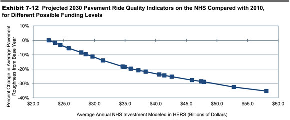
| Minimum BCR Cutoff | HERS-Modeled NHS Capital Investment 1 2 | Projected Impact of HERS-Modeled Capital Investment on the NHS1 | |||||
|---|---|---|---|---|---|---|---|
| Computed Average Annual Percent Change in Spending 3 |
Average Annual Spending (Billions of 2010 Dollars) Total |
Average Annual Spending (Billions of 2010 Dollars) System Rehabilitation 4 |
Percent of 2030 VMT on Roads With...5 IRI<95 |
Percent of 2030 VMT on Roads With...5 IRI<170 |
Average IRI Projected 2030 Level |
Average IRI Change Relative to Base Year |
|
| 1.00 | 3.30% | $58.1 | $24.0 | 89.6% | 96.7% | 69.0 | -35.3% |
| 1.50 | 1.17% | $45.9 | $20.0 | 83.5% | 94.9% | 77.1 | -27.7% |
| 1.78 | 0.00% | $40.6 | $18.2 | 80.2% | 93.9% | 81.3 | -23.7% |
| 2.19 | -1.54% | $34.6 | $16.0 | 75.6% | 92.6% | 87.2 | -18.2% |
| 2.49 | -2.51% | $31.4 | $14.7 | 72.2% | 91.7% | 91.7 | -14.0% |
| 2.73 | -3.73% | $27.9 | $13.2 | 67.7% | 90.5% | 97.6 | -8.4% |
| 2.88 | -6.01% | $22.5 | $11.2 | 61.6% | 88.8% | 106.6 | 0.0% |
| Base Year Values: | 54.7% | 88.8% | 106.6 | ||||
2 The seven NHS capital investment levels identified were derived from systemwide HERS runs with the minimum BCR cutoff identified in the first column, based on the portion of these runs directed to the NHS. While the systemwide capital investment for these runs grew at a constant annual rate, this was not the case for the subset of the total spending that was directed to the NHS.
3 The amounts shown represent the average annual growth rate in NHS spending that would generate a cumulative 20-year spending level consistent with the average annual HERS-modeled NHS investment levels identified in the third column. The HERS runs were not actually developed using these growth rates.
4 The portion of HERS-modeled spending directed toward system rehabilitation varies by funding level and is not directly linked to actual spending for this purpose in the baseline year.
5 As discussed in Chapter 3, IRI values of 95 and 170 inches per mile, respectively, are the thresholds associated with “good” and “acceptable” pavement ride quality on the NHS. The base year values shown are 2010 values reported in Chapter 3, rather than those reflected in the 2008 HPMS sample data set.
At the other end of the investment spectrum in Exhibit 7-12, implementing all cost-beneficial improvements would require annual average spending on the NHS estimated at $58.1 billion, which is projected to reduce the average IRI over the analysis period by 35.3 percent. At this level of investment in the system, the model also projects that pavements with an IRI below 95, which was the criterion in Chapter 3 for rating ride quality as “good”, will carry 89.6 percent of the VMT on the NHS, up from the 54.7 percent estimated for 2010. Based on these modeling results, additional investment to bring this percentage closer to 100 percent would be economically inefficient, as the costs would exceed the benefits.
Impact of Future Investment on NHS Travel Times and User Costs
Exhibit 7-13 presents the projections of NHS averages for time-related indicators of performance, along with the amount that HERS programs for NHS expansion projects (which more than preservation projects affect these indicators). For HERS to project average speed on the NHS to be the unchanged from 2010 to 2030, an annual average of $31.4 billion of NHS spending would be required, a level that could be achieved if annual NHS spending declines by 2.51 percent per year. In contrast, when average annual investment on the NHS is what would be needed to implement all cost-beneficial improvements, an estimated $58.1 billion, HERS projects average NHS speed to be 4.4 percent higher in 2030 than in 2010 (50.8 mph versus 48.7 mph). At this investment level, HERS also projects for the NHS that average delay will decline by 18.4 percent, and average user cost by 2.4 percent, over the analysis period. For the case where investment in the NHS would remain at the 2010 level, average delay decreases by 5.9 percent, while average user costs are projected to decrease by 0.6 percent.
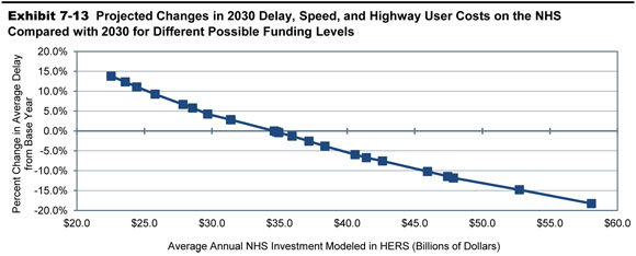
| Minimum BCR Cutoff | HERS-Modeled NHS Capital Investment 1 | Projected Impact of HERS-Modeled Capital Investment on the NHS 1 | |||||
|---|---|---|---|---|---|---|---|
| Computed Average Annual Percent Change in Spending |
Average Annual Spending (Billions of 2010 Dollars) Total |
Average Annual Spending (Billions of 2010 Dollars) System Expansion2 |
Percent Change Relative to Baseline per VMT Average User Costs |
Percent Change Relative to Baseline per VMT Average Delay |
Average Speed Projected 2030 Level (mph) |
Average Speed Change Relative to Base Year |
|
| 1.00 | 3.30% | $58.1 | $34.1 | -2.4% | -18.3% | 50.8 | 4.4% |
| 1.50 | 1.17% | $45.9 | $25.9 | -1.2% | -10.2% | 50.0 | 2.7% |
| 1.78 | 0.00% | $40.6 | $22.4 | -0.6% | -5.9% | 49.6 | 1.9% |
| 2.19 | -1.54% | $34.6 | $18.6 | 0.2% | 0.0% | 49.0 | 0.6% |
| 2.49 | -2.51% | $31.4 | $16.7 | 0.7% | 2.8% | 48.7 | 0.0% |
| 2.73 | -3.73% | $27.9 | $14.6 | 1.5% | 6.7% | 48.3 | -0.9% |
| 2.88 | -6.01% | $22.5 | $11.4 | 2.7% | 13.8% | 47.5 | -2.5% |
| Base Year Value: | 48.7 | ||||||
2 The portion of HERS-modeled spending directed toward system expansion varies by funding level and is not directly linked to actual spending for this purpose in the baseline year. System expansion expenditures have a more direct impact on delay and speed, while both system expansion and system rehabilitation expenditures impact highway user costs.
Impacts of Interstate System Investments Modeled by HERS
The Interstate System, unlike the broader NHS of which it is a part, has standard design and signing requirements, which makes it the most recognizable subset of the highway network. This section examines the amount of investment that HERS directs to the Interstate System, and the potential impacts of this investment on future Interstate System conditions and performance. For this analysis, the funding levels presented were selected in the same way as those for the preceding section’s analysis of investment in the NHS.
| How were the seven Interstate System investment levels presented in Exhibits 7-14 and 7-15 selected? | |
|
The investment levels associated with minimum BCR cutoffs of 1.00 and 1.50 were derived from the same HERS runs identified in Exhibit 7-3 as associated with these cutoffs assuming VMT growth consistent with the HPMS-derived forecast. The investment levels shown reflect the portion of spending in those runs that was directed to the Interstate System.
The remaining five levels were selected using comparable criteria to those identified in Exhibit 7-3, but in terms of the Interstate System in particular, rather than Federal-aid highways in general. The 20-year investment level associated with a minimum BCR cutoff of 2.72 results in an average annual investment level of $14.7 billion, consistent with spending on the Interstate System in 2010 on types of capital improvements modeled in HERS. The investment level associated with a minimum BCR cutoff of 2.66 was selected to be included because it results in projected average speed in 2030 matching the base year level. Investing at the level associated with a minimum BCR cutoff of 2.70 is projected to result in average delay being maintained, while applying a minimum BCR cutoff of 2.97 would maintain average IRI. The minimum BCR cutoff of 2.84 was selected as it results in a level of Interstate System spending that equals the average of the levels associated with maintaining average delay and maintaining average IRI. |
|
Impact of Future Investment on Interstate Pavement Ride Quality
Exhibit 7-14 shows the levels of Federal-aid highway investment that HERS allocates to the Interstate System. To throw light on the projections for Interstate System pavement, the exhibit also shows the portion of modeled Interstate System spending that HERS allocates to system rehabilitation projects. At the assumed level of Federal-aid investment that would cause HERS to allocate to the Interstate System an annual average of $14.7 billion, matching the level invested in 2010, the model projects average pavement roughness on the Interstate System to be 12.7 lower in 2030 than in 2010. For HERS to project average pavement roughness to remain unchanged between these years would require assuming a level of Federal-aid highway investment out of which the model would allocate to the Interstate System an annual average of $11.1 billion, which could be achieved with an average annual reduction in spending of 2.71 percent per year starting in 2010.
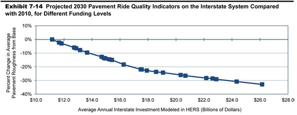
| Minimum BCR Cutoff | HERS-Modeled Interstate Capital Investment 1 | Projected Impact of HERS-Modeled Capital Investment on the Interstate System | |||||
|---|---|---|---|---|---|---|---|
| Computed Average Annual Percent Change in Spending2 |
Average Annual Spending (Billions of 2010 Dollars) Total |
Average Annual Spending (Billions of 2010 Dollars) System Rehabilitation 3 |
Percent of 2030 VMT on Roads With...4 IRI<95 |
Percent of 2030 VMT on Roads With...4 IRI<170 |
Average IRI Projected 2030 Level |
Average IRI Change Relative to Base Year |
|
| 1.00 | 5.22% | $26.2 | $8.5 | 94.2% | 99.6% | 62.3 | -32.9% |
| 1.50 | 3.77% | $22.2 | $7.7 | 90.8% | 98.9% | 66.6 | -28.2% |
| 2.66 | 0.35% | $15.2 | $5.9 | 81.6% | 96.5% | 79.3 | -14.5% |
| 2.70 | 0.17% | $15.0 | $5.9 | 81.0% | 96.3% | 79.9 | -13.9% |
| 2.72 | 0.00% | $14.7 | $5.8 | 80.3% | 96.2% | 81.0 | -12.7% |
| 2.84 | -1.28% | $12.9 | $5.3 | 76.8% | 95.4% | 86.8 | -6.5% |
| 2.97 | -2.71% | $11.1 | $4.6 | 72.1% | 94.4% | 92.8 | 0.0% |
| Base Year Values: | 69.5% | 90.3% | 92.8 | ||||
2The amounts shown represent the average annual growth rate in Interstate System spending that would generate a cumulative 20-year spending level consistent with the average annual HERS-modeled Interstate System investment levels identified in the third column. The HERS runs were not actually developed using these growth rates.
3 The portion of HERS-modeled spending directed toward system rehabilitation varies by funding level and is not directly linked to actual spending for this purpose in the baseline year.
4 As discussed in Chapter 3, IRI values of 95 and 170 inches per mile, respectively, are the thresholds associated with “good” and “acceptable” pavement ride quality on the NHS. The base year values shown are based on 2010 values reported in Chapter 3, rather than those reflected in the 2008 HPMS sample data set.
At the other end of the investment spectrum in Exhibit 7-14, implementing all cost-beneficial improvements would require annual average spending on the Interstate System estimated at $26.2 billion; this level of investment is projected to reduce the average IRI over the analysis period by 32.9 percent. At this economically efficient level of investment in the Interstate System, the model also projects that pavements with an IRI below 95, which was the criterion in Chapter 3 for rating ride quality as “good”, will carry 94.2 percent of the VMT on the Interstate System, up from the 69.5 percent estimated for 2010.
Impact of Future Investment on Interstate System Travel Times and User Costs
Exhibit 7-15 presents the projections of Interstate System averages for time-related indicators of performance, along with the amount that HERS programs for Interstate System expansion projects. For HERS to project average speed on the Interstate System to be unchanged from 2010 to 2030, an annual average of $15.2 billion of Interstate System spending would be required, which could be achieved if spending increases by 0.35 percent per year beginning in 2010. In contrast, when average annual investment in the Interstate System is what would be needed to implement all cost-beneficial improvements, an estimated $26.2 billion, HERS projects average Interstate System speed to be 7.5 percent higher in 2030 than in 2010 (64.6 mph versus 60.1 mph). At this investment level, HERS also projects for the Interstate System that average congestion delay will decline by 39.5 percent, and average user cost by 2.9 percent, over the analysis period. For the case where investment in the Interstate System would remain at the 2010 level, average congestion delay and average user cost are each projected to decrease by about one percent.
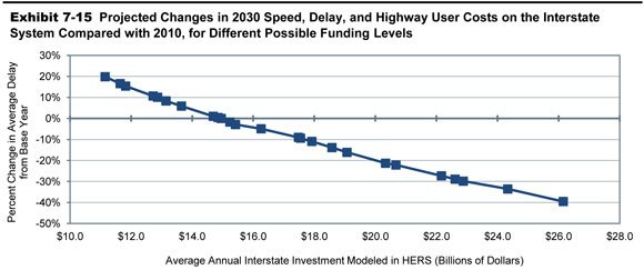
| Minimum BCR Cutoff | HERS-Modeled Interstate Capital Investment | Projected Impact of HERS-Modeled Capital Investment on the Interstate System | |||||
|---|---|---|---|---|---|---|---|
| Computed Average Annual Percent Change in Spending |
Average Annual Spending (Billions of 2008 Dollars) Total |
Average Annual Spending (Billions of 2008 Dollars) System Expansion1 |
Percent Change Relative to Baseline per VMT Average User Costs |
Percent Change Relative to Baseline per VMT Average Delay |
Average Speed Projected 2030 Level (mph) |
Average Speed Change Relative to Baseline |
|
| 1.00 | 5.22% | $26.2 | $17.6 | -2.9% | -39.5% | 64.6 | 7.5% |
| 1.50 | 3.77% | $22.2 | $14.5 | -1.9% | -27.3% | 63.1 | 5.0% |
| 2.66 | 0.35% | $15.2 | $9.3 | 0.6% | -1.7% | 60.1 | 0.0% |
| 2.70 | 0.17% | $15.0 | $9.1 | 0.8% | 0.0% | 60.0 | -0.3% |
| 2.72 | 0.00% | $14.7 | $8.9 | 0.9% | 1.0% | 59.8 | -0.5% |
| 2.84 | -1.28% | $12.9 | $7.6 | 2.0% | 10.1% | 58.6 | -2.5% |
| 2.97 | -2.71% | $11.1 | $6.5 | 3.1% | 19.8% | 57.6 | -4.2% |
| Base Year Values: | 60.1 | ||||||
National Bridge Investment Analysis System
The scenario estimates relating to bridge repair and replacement shown in this report are derived primarily from NBIAS, which accepts detailed structural data on individual bridge elements. Because such detailed information is not currently available at the national level, NBIAS also has the capability to synthesize element level data from the general condition ratings reported for individual bridges in the National Bridge Inventory (NBI). The analyses presented in this report are based on synthesized element level data. Examples of bridge elements include the bridge deck, a steel girder used for supporting the deck, a concrete pier cap on which girders are placed, a concrete column used for supporting the pier cap, or a bridge railing.
The NBIAS model uses a probabilistic approach to model bridge deterioration for each synthesized bridge element. It relies on a set of transition probabilities to project the likelihood that an element will deteriorate from one condition state to another over a given period of time. Another key input to the model is the overall objective assumed for maintenance, repair, and rehabilitation (MR&R) policies. Previous C&P reports assumed that the bridge owners would follow MR&R policies aimed at minimizing costs, but NBIAS has recently been enhanced to allow alternative assumptions. In this report, the standard assumption is that bridge owners will pursue MR&R policies aimed at achieving a steady state of bridge performance; other assumptions are considered for sensitivity analysis in Chapter 10. Given the assumed policy objective, NBIAS determines an optimal set of MR&R actions to take for each bridge element based on the condition of the element.
To estimate functional improvement needs, NBIAS applies a set of improvement standards and costs to each bridge in the NBI. The model then identifies potential improvements—such as widening existing bridge lanes, raising bridges to increase vertical clearances, and strengthening bridges to increase load-carrying capacity—and evaluates their potential benefits and costs. NBIAS evaluates potential bridge replacements by comparing their benefits and costs with what could be achieved through MR&R work alone. Appendix B discusses the NBIAS model in more detail.
In using the NBIAS model to project conditions and performance of the Nation’s bridges over 20 years, this section considers the alternatives of continuing to invest in bridge rehabilitation at the 2010 level (in constant dollars) and at higher or lower levels. The expenditures modeled pertain only to bridge system rehabilitation; expenditures associated with bridge system expansion are modeled separately as part of the capacity expansion analysis in the HERS model. (The NBIAS-modeled investments presented here should be considered as additive to the HERS-modeled investments presented above; each of the capital investment scenarios presented in Chapter 8 combines one of the HERS analyses with one of the NBIAS analyses, and makes adjustments to account for non-modeled spending.)
Performance Measures
The NBIAS model considers bridge deficiencies at the level of individual bridge elements based on engineering criteria and computes an initial value for the cost of a set of corrective actions that would address all such deficiencies. The economic bridge investment backlog represents the combined cost of these corrective actions in those cases where NBIAS estimates it would be cost-beneficial to implement them. Changes in this economic bridge investment backlog over time can be viewed as a proxy for changes in overall bridge conditions.
Previous editions of the C&P report used the economic bridge investment backlog as the sole indicator of bridge system performance. For a more comprehensive view of the impacts of various levels of investment, two new additional metrics have been added for this edition, the average Sufficiency Rating and the average Health Index.
| How does the NBIAS definition of bridge deficiencies compare with the information on structurally deficient bridges reported in Chapter 3? | |
|
NBIAS considers bridge deficiencies and corrective improvements at the level of individual bridge elements. The economic backlog of bridge deficiencies estimated by NBIAS thus consists of the cost of all improvements to bridge elements that would be justified on both engineering and economic grounds. It includes many improvements on bridges with certain components that may warrant repair, rehabilitation, or replacement, but whose overall condition is not sufficiently deteriorated for them to be classified as structurally deficient.
The corrective actions recommended by NBIAS would include those aimed at addressing structural deficiencies, as well as some functional deficiencies. System expansion needs for both highways and bridges are addressed separately as part of the HERS model analysis. |
|
Prior to MAP-21, under the Highway Bridge Program (HBP), the Sufficiency Rating of a bridge served as a factor for determining funding eligibility and as an initial prioritization. This initial prioritization, which was provided annually to the States and known as the “Selection List,” was a listing of bridges that were eligible for programming for replacement and rehabilitation (other activities under the HBP with separate and different eligibility criteria such as systematic preventive maintenance were also eligible for programming). The Sufficiency Rating is a numeric value that ranges from 100 to 0, in which 100 represents an entirely sufficient bridge and 0 represents an entirely insufficient or deficient bridge. Its calculation is based on a complex formula involving a number of NBI data fields relating to: structural adequacy and safety (in terms of bridge component condition ratings and a load capacity rating), serviceability and functional obsolescence (in terms of bridge geometric features and appraisal ratings, volume of traffic carried, approach roadway features, deck condition rating, structural evaluation, and whether the bridge is on the Strategic Highway Network [STRAHNET]), and essentiality for public use (in terms of volume of traffic carried, detour length, and whether the bridge is on the STRAHNET). For this report, the investment scenarios presented in Chapter 8 focus on the Sufficiency Rating rather than the economic bridge investment backlog.
The Bridge Health Index is a 0-100 ranking system typically used in the context of decision making for bridge preventative maintenance. Although element condition states are categorical; it is useful to think of the condition of an element at a given time as a point along a continuous timeline from 100 percent in the best state to 100 percent in the worst state. The Health Index merely indicates where the element is along this continuum. To aggregate the element-level result to the bridge level, weights are assigned to the elements according to the economic consequences of element failure. Thus, elements whose failure has relatively little economic effect, such as railings, receive less weight than elements whose failure could close the bridge, such as girders. In general, the lower the Health Index number, the higher the priority for rehabilitation or maintenance of the structure, though other factors also come into play when determining priority of work on bridges.
Impacts of Systemwide Investments Modeled by NBIAS
As referenced in Chapter 6, of the $100.2 billion invested in highways in 2010, $17.1 billion was used for bridge system rehabilitation, an increase of more than one-third compared to 2008. This sharp increase is attributable in part to the use of Recovery Act funds to repair and replace bridges.
For investments of the types modeled by NBIAS, Exhibit 7-16 shows how the total amount invested over the 20-year analysis period influences the bridge performance levels projected for the final year, 2030. If spending were sustained at its 2010 level in constant dollar terms, projected performance for 2030 would improve relative to 2010 for each of the three measures considered. The average Sufficiency Rating would increase from 81.7 in 2010 to 84.1 in 2030, the average Health Index would rise from 92.1 to 92.7; and the economic investment backlog would decrease by 92.6 percent relative to its 2010 level of $106.4 billion. The highest level of spending shown in Exhibit 7-16 averages $20.2 billion per year, which is the estimate of what would be needed to eliminate the economic backlog by 2030.
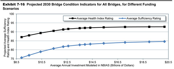
| NBIAS-Modeled Capital Investment | Projected Impact of NBIAS-Modeled Capital Investment | ||||
|---|---|---|---|---|---|
| Annual Percent Change in Spending | Average Annual Spending1 (Billions of 2010 Dollars) |
2030 Average Sufficiency Rating |
2030 Average Health Index |
Economic Investment Backlog2 2030 (Billions of 2010 Dollars) |
Economic Investment Backlog 2 Change Relative to Baseline |
| 1.57% | $20.2 | 84.6 | 92.8 | $0.0 | -100.0% |
| 0.00% | $17.1 | 84.1 | 92.7 | $7.9 | -92.6% |
| -1.70% | $14.3 | 83.2 | 92.3 | $20.6 | -80.6% |
| -2.30% | $13.5 | 82.7 | 92.1 | $26.4 | -75.2% |
| -3.33% | $12.2 | 81.7 | 91.3 | $39.5 | -62.9% |
| -6.72% | $8.9 | 75.6 | 87.1 | $106.4 | 0.0% |
| 2010 Baseline Values: | 81.7 | 92.1 | $106.4 | ||
2 The amounts shown do not reflect system expansion needs; the bridge components of such needs are addressed as part of the HERS model analysis.
Exhibit 7-16 also indicates that bridge investment spending could be reduced from the 2010 level while maintaining bridge performance. If average annual spending declined by 2.30 percent to an average annual investment level of $13.5 billion, this would still be sufficient to maintain the average Health Index at its 2010 level through 2030. An annual decrease in investment of 3.33 percent to an average investment level of $12.2 billion would be adequate to maintain the average Sufficiency Rating at its 2010 level. The economic bridge investment backlog could be maintained at its 2010 level even if annual bridge investment declined by 6.72 percent per year to an average annual level of $8.9 billion.
| Why does the economic backlog estimated by NBIAS differ from bridge backlog figures estimated by some other organizations? | |
|
One major reason for such differences is that the backlog estimated by NBIAS is not intended to constitute a complete bridge investment estimate backlog. The NBIAS figures relate only to investment needs associated with the condition of existing structures, and not capacity expansion needs. The backlog estimated by HERS includes estimates of capacity-related needs for highways and bridges combined.
Some estimates of bridge backlog produced by other organizations do attempt to combine estimates of needs relating to bridge capacity with those relating to existing structures. |
|
Impacts of Federal-Aid Highway Investments Modeled by NBIAS
For bridges on Federal-aid highways, Exhibit 7-17 compares performance projections for 2030 at various levels of investment with measured performance in 2010. If spending on types of improvements modeled in NBIAS were sustained at the 2010 level of $12.5 billion (in constant dollars), the projections show performance improving. The average Sufficiency Rating would increase from 82.0 in 2010 to 83.6 in 2030 and the average Health Index would rise from 92.0 to 92.5; the economic investment backlog would decrease by 84.8 percent from its 2010 level of $86.8 billion. If spending increases by 2.61 percent per year to an average annual level of $16.6 billion, the economic investment backlog would fall to zero by 2030, while the average Sufficiency Rating would increase to 84.7 and the average Health Index would increase to 92.9.
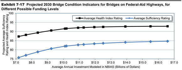
| NBIAS-Modeled Capital Investment on Federal-Aid Highway Bridges |
Projected Impact of NBIAS-Modeled Capital Investment on Federal-Aid Highway Bridges | ||||
|---|---|---|---|---|---|
| Annual Percent Change in Spending | Average Annual Spending1 (Billions of 2010 Dollars) |
2030 Average Sufficiency Rating |
2030 Average Health Index |
Economic Investment Backlog 2 2030 (Billions of 2010 Dollars) |
Economic Investment Backlog 2 Change Relative to Baseline |
| 2.61% | $16.6 | 84.7 | 92.9 | $0.0 | -100.0% |
| 0.00% | $12.5 | 83.6 | 92.5 | $13.2 | -84.8% |
| -0.44% | $12.0 | 83.3 | 92.4 | $16.2 | -81.3% |
| -1.31% | $10.9 | 82.7 | 92.0 | $22.8 | -73.7% |
| -2.09% | $10.1 | 82.0 | 91.6 | $30.8 | -64.5% |
| -5.67% | $7.2 | 75.7 | 87.3 | $86.8 | 0.0% |
| 2010 Baseline Values: | 82.0 | 92.0 | $86.8 | ||
2 The amounts shown do not reflect system expansion needs; the bridge components of such needs are addressed as part of the HERS model analysis.
If spending declined by 1.31 percent per year to an average annual investment level of $10.9 billion, this would still be sufficient to maintain the average Health Index at its 2010 level through 2030. An annual decrease in investment of 2.09 percent to an average investment level of $10.1 billion would be adequate to maintain the average Sufficiency Rating at its 2010 level. The economic bridge investment backlog could be maintained at its 2010 level even if annual bridge investment declined by 5.67 percent per year to an average annual level of $7.2 billion.
Impacts of NHS Investments Modeled by NBIAS
Exhibit 7-18 shows the impact of varying funding levels on the performance of bridges on the NHS. As noted earlier, the NHS analyses presented in this chapter are based on an estimate of what the NHS will look like after it is expanded pursuant to MAP-21, rather than the actual system as it existed in 2010.
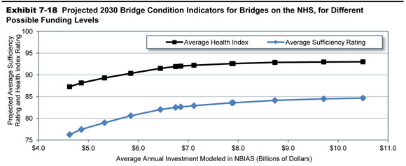
| NBIAS-Modeled Capital Investment on NHS Bridges1 |
Projected Impact of NBIAS-Modeled Capital Investment on NHS Bridges1 | ||||
|---|---|---|---|---|---|
| Annual Percent Change in Spending | Average Annual Spending2 (Billions of 2010 Dollars) |
2030 Average Sufficiency Rating |
2030 Average Health Index |
Economic Investment Backlog 3 2030 (Billions of 2010 Dollars) |
Economic Investment Backlog 2 Change Relative to Baseline |
| 1.72% | $10.5 | 84.7 | 93.0 | $0.0 | -100.0% |
| 0.00% | $8.7 | 84.1 | 92.9 | $4.9 | -91.7% |
| -0.97% | $7.9 | 83.6 | 92.6 | $10.3 | -82.6% |
| -2.38% | $6.8 | 82.6 | 92.0 | $18.9 | -68.2% |
| -2.53% | $6.7 | 82.5 | 91.9 | $19.9 | -66.4% |
| -6.55% | $4.6 | 76.3 | 87.3 | $59.2 | 0.0% |
| 2010 Baseline Values: | 82.5 | 92.0 | $59.2 | ||
2 The amounts shown represent the average annual investment over 20 years by all levels of government combined that would occur if annual investment grows in constant dollar terms by the percentage shown in each row of the first column. Bridges on roadways functionally classified as rural minor collector, rural local, and urban local are not included in these figures.
3 The amounts shown do not reflect system expansion needs; the bridge components of such needs are addressed as part of the HERS model analysis.
If spending on types of improvements modeled in NBIAS on NHS bridges were sustained at the 2010 level of $8.7 billion in constant dollar terms, projected performance for 2030 would improve relative to 2010. The average Sufficiency Rating would increase from 82.5 in 2010 to 84.1 in 2030, the average Health Index would rise from 92.0 to 92.9, and the economic investment backlog would decrease by 91.7 percent relative to its 2010 level of $59.2 billion. If spending were to increase by 1.72 percent per year to an average annual level of $10.5 billion, this is estimated to be sufficient to reduce the economic investment backlog to zero by 2030, while increasing the average Sufficiency Rating to 84.7 and increasing the average Health Index to 93.0.
If spending declined by 2.38 percent per year to an average annual investment level of $6.8 billion, this would still be sufficient to maintain the average Health Index at its 2010 level through 2030. An annual decrease in investment of 2.53 percent to an average investment level of $6.7 billion would be adequate to maintain the average Sufficiency Rating at its 2010 level. The economic bridge investment backlog could be maintained at its 2010 level even if annual bridge investment declined by 6.55 percent per year to an average annual level of $4.6 billion.
Impacts of Interstate Investments Modeled by NBIAS
Exhibit 7-19 shows the impact of varying funding levels on the performance of those bridges on the Interstate System. If spending on types of improvements modeled in NBIAS on Interstate bridges were sustained at the 2010 level of $4.1 billion in constant dollar terms, projected performance for 2030 would improve relative to 2010. The average Sufficiency Rating would increase from 82.3 in 2010 to 84.0 in 2030, the average Health Index would rise from 91.7 to 92.9, and the economic investment backlog would decrease by 91.4 percent relative to its 2010 level of $30.4 billion. If spending were to increase by 1.23 percent per year to an average annual level of $4.7 billion, this is estimated to be sufficient to reduce the economic investment backlog to zero by 2030, while increasing the average Sufficiency Rating to 84.5 and increasing the average Health Index to 93.1.

| NBIAS-Modeled Capital Investment on Interstate Bridges |
Projected Impact of NBIAS-Modeled Capital Investment on Interstate Bridges | ||||
|---|---|---|---|---|---|
| Annual Percent Change in Spending | Average Annual Spending1 (Billions of 2010 Dollars) |
2030 Average Sufficiency Rating |
2030 Average Health Index |
Economic Investment Backlog 2 2030 (Billions of 2010 Dollars) |
Economic Investment Backlog 2 Change Relative to Baseline |
| 1.23% | $4.7 | 84.5 | 93.1 | $0.0 | -100.0% |
| 0.00% | $4.1 | 84.0 | 92.9 | $2.6 | -91.4% |
| -0.93% | $3.7 | 83.4 | 92.6 | $5.7 | -81.1% |
| -2.20% | $3.3 | 82.3 | 91.9 | $11.3 | -62.7% |
| -2.60% | $3.2 | 82.0 | 91.7 | $12.8 | -57.7% |
| -5.94% | $2.3 | 76.8 | 87.7 | $30.4 | 0.0% |
| 2010 Baseline Values: | 82.3 | 91.7 | $30.4 | ||
2 The amounts shown do not reflect system expansion needs; the bridge components of such needs are addressed as part of the HERS model analysis.
If annual spending declined by 2.20 percent per year to an average annual investment level of $3.3 billion, this would still be adequate to maintain the average Sufficiency Rating at its 2010 level through 2030. An annual decrease in investment of 2.60 percent to an average investment level of $3.2 billion would be sufficient to maintain the average Health Index at its 2010 level. The economic bridge investment backlog could be maintained at its 2010 level even if annual bridge investment declined by 5.94 percent per year to an average annual level of $2.3 billion.
Potential Transit Capital Investment Impacts
This section examines how different types and levels of annual capital investments would likely affect transit system condition and performance by the year 2030. It begins with an overview of the types of capital spending projected by the Federal Transit Administration’s (FTA’s) Transit Economic Requirements Model (TERM), which is the primary analysis tool used to assess transit investment needs and impacts in Part II of this report. The section then examines how variations in the level of annual capital spending are likely to impact future transit conditions and performance—both at the national level and for urbanized areas (UZAs) with populations greater than 1 million.
Types of Capital Spending Projected by TERM
TERM is an analysis tool that uses engineering and economic concepts to forecast total capital investment needs for the U.S. transit industry through a 20-year time horizon. Specifically, TERM is designed to forecast the following types of investment needs:
- Preservation: The level of investment in the rehabilitation and replacement of existing transit capital assets required to attain specific investment goals (e.g., to attain a state of good repair [SGR]) subject to potentially limited capital funding.
- Expansion: The level of investment in the expansion of transit fleets, facilities, and rail networks required to support projected growth in transit demand (i.e., maintain performance at current levels as demand for service increases).
TERM includes a benefit-cost test that is applied to expansion scenarios to determine which investments are cost effective and which are not; TERM reports investment costs only for investments that pass the test. The SGR benchmark, described in Chapter 8, uses a zero-growth assumption and turns off the cost-benefit test. It estimates the cost of maintaining what is currently in service as an analytical exercise and is not considered to be a realistic scenario.
The data used to support TERM’s needs estimates are derived from a variety of sources—including asset inventory data provided by local transit agencies (at FTA’s request), fleet investment and transit performance data obtained from the National Transit Database (NTD), and transit travel demand forecast data provided by metropolitan planning organizations (MPOs). Appendix C contains a detailed description of the analysis methodology used by TERM.
Preservation Investments
TERM estimates current and future preservation investment needs by first assessing the age and current condition of the Nation’s existing stock of transit assets (the results of this analysis were presented in Chapter 3 of this report). TERM then uses this information to assess both current reinvestment needs (i.e., the reinvestment backlog) as well as the expected level of ongoing investment required to meet the life-cycle needs of the Nation’s transit assets over the next 20 years, including all required rehabilitation and replacement activities.
Condition-Based Reinvestment. Rather than relying on age alone in assessing the timing and cost of current and future reinvestment activities, TERM uses a set of empirical asset deterioration curves that estimate asset condition (both current and future) as a function of asset type, age, past rehabilitation activities, and possibly past maintenance and utilization levels (depending on asset type). The timing of specific rehabilitation and replacement activities is determined by an asset’s estimated condition at the start of each year over the 20-year forecast horizon, with asset condition declining as the asset ages, triggering reinvestment events at different levels of deterioration and leading ultimately to outright replacement.
Financial Constraints, the Investment Backlog, and Future Conditions. TERM is designed to estimate investment needs with or without annual capital funding constraints. When run without funding constraints, TERM estimates the total level of investment required to complete all of the rehabilitation and replacement needs identified by the model at the time when those investment needs come due (hence, there is no appreciable investment backlog with unconstrained analyses after any initial deferred investment is addressed). In contrast, when TERM is run in a financially constrained mode, there may not be sufficient funding to cover the reinvestment needs of all assets, in which case some reinvestment activities are deferred until a future period when sufficient funds become available. The lack of sufficient funds to address all reinvestment needs for some or all years of the 20-year model results in varying levels of investment backlog during this time period. Most analyses presented in this chapter were completed using funding constraints. Similarly, TERM’s ability to estimate asset conditions—both current and future—allows for assessment of how future asset conditions are likely to improve or decline given varying levels of capital reinvestment. Finally, note that TERM’s benefit-cost analysis is utilized to determine the order in which reinvestment activities are completed when funding capacity is limited, with investments with the highest benefit-cost ratios addressed first.
Expansion Investments
In addition to ongoing reinvestment in existing assets, most transit agencies also invest in the expansion of their vehicle fleets, maintenance facilities, fixed guideway, and other assets. Investments in expansion assets can be thought of as serving two distinct purposes. First, the demand for transit services typically increases over time in line with population growth, employment, and other factors. To maintain current levels of performance in the face of expanding demand, transit operators must similarly expand the capacity of their services (e.g., by increasing the number of vehicles in their fleets). Failure to accommodate this demand would result in increased vehicle crowding, increased dwell times at passenger stops, and decreased operating speeds for existing services. Second, transit operators also invest in expansion projects with the aim of improving current service performance. Such improvements include capital expansion projects (e.g., a new light rail segment) to reduce vehicle crowding or increase average operating speeds. TERM is designed to assess investment needs and impacts for both types of expansion investments.
Expansion Investments: Maintain Performance
To assess the level of investment required to maintain existing service quality, TERM estimates the rate of growth in transit vehicle fleets required to maintain current vehicle occupancy levels given the projected growth rate in transit passenger miles. In addition to assessing the level of investment in new fleet vehicles required to support this growth, TERM also forecasts investments in the expansion of other assets needed to support projected fleet growth, including bus maintenance facilities and, in the case of rail systems, additional investment in guideway, track work, stations, maintenance facilities, train control, and traction power systems. Asset expansion investment needs are assessed for all agencies reporting to the NTD on a mode-by-mode basis. However, cost-benefit constraints prevent TERM from investing in asset expansion for those agency-modes with low ridership (per vehicle) as compared with the national average.
Expansion Investments: Improve Performance
In prior editions of the C&P report, TERM was used to estimate the level of investment required to improve current transit performance by (1) reducing crowding in higher-utilization transit systems and (2) expanding existing investment in rail as a means of improving average operating speeds in urbanized areas with average operating speeds (across all transit modes) well below the national average. For this edition, the impact of increased investment on system performance is assessed by developing TERM scenarios where the rate of investment in transit asset expansion exceeds the projected rate of growth in transit passenger miles. This difference between the rate of asset expansion and actual growth in travel demand represents projected long-term reductions in in-vehicle crowding and potential increases in average operating speed.
Recent Investment in Transit Preservation and Expansion
Exhibit 7-20 shows the broad composition of the 2010 spending by U.S. transit agencies on capital projects that correspond to the investment types modeled in TERM. Of the total spending amounting to $16.5 billion, $10.3 billion or 62.5 percent was devoted to preserving existing assets, and the rest was spent on expansion investments.
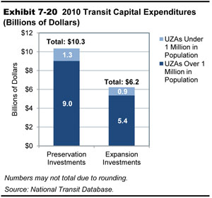
As expected, preservation and expansion spending were concentrated in the large urban systems. In combination, urbanized areas with populations greater than 1 million in 2010 accounted for 87.1 percent of preservation spending and 86.1 percent of expansion spending. Smaller urbanized areas and rural areas accounted for the rest.
Impacts of Systemwide Investments Modeled by TERM
This section uses TERM analyses to assess how different levels of investment in the preservation and expansion of the Nation’s transit asset base can be expected to impact transit conditions and performance over the next 20 years. A key objective here is to place a broad range of potential future investment levels—and the consequences of those levels of investment—within the context of both the current expenditures on transit preservation and expansion and of some potential investment goals (e.g., attainment of an SGR within 20 years). More specifically, these analyses consider the impact of different levels of transit capital expenditures on the following:
- Preservation Investments—Average condition rating of U.S. transit assets and state of good repair backlog
- Expansion Investments—Additional ridership (boardings) capacity.
Each of these analyses is completed first at the national level (the remainder of this section) and then repeated (in the following section) for two different segments of urbanized areas, including the following:
- Urbanized areas with populations greater than 1 million
- All other urbanized areas and rural areas with existing transit services.
Impact of Preservation Investments on Transit Backlog and Conditions
This subsection considers the expected impact of varying levels of aggregate capital reinvestment by all levels of government on the future investment backlog and physical condition (as of 2030) for the Nation’s existing stock of transit assets.
Transit Backlog. The 2010 Conditions and Performance Report introduced the concept of reinvestment backlog as an indication of the amount of near-term investment needed to replace assets that are past their expected useful lifetime. It focuses attention on assets that are in the worst condition rather than on the average condition of all assets, which is reported below and has been the primary measure in previous editions. This additional perspective is needed since average condition has become less meaningful in the current environment with high levels of investment in new assets for transit system expansion. Investment backlog is a measure of the need for investment in infrastructure preservation. TERM estimates that investment backlog is $85.9 billion (see Chapter 8).
Exhibit 7-21 focuses on the impact of future spending levels on this investment backlog. Specifically, Exhibit 7-21 presents the estimated impact of differing levels of annual capital reinvestment on the expected size of the investment backlog in 2030. The investment backlog is defined here as the level of investment required to bring all of the Nation’s assets to a state of good repair. This includes replacement of those assets that currently exceed their useful lives (the $85.9 billion) and the performance of all major rehabilitation activities and replacement of assets that will exceed their useful lives during the analysis period. If future reinvestment rates are insufficient to address these ongoing reinvestment needs as they arise, then the size of the backlog will increase over time. Reinvestment at a rate above that required to address new needs as they arise will ultimately result in elimination of the existing backlog.
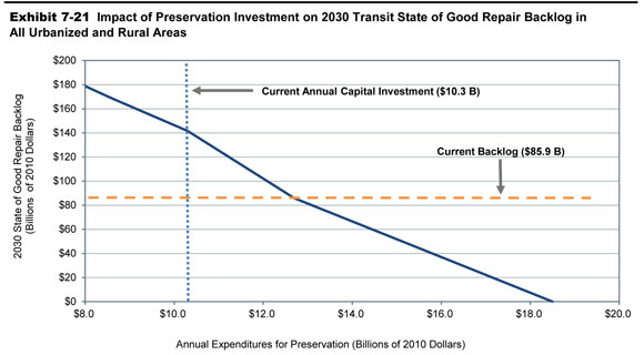
| Average Annual Investment (Billions of 2010 Dollars) | Average Annual Percent Change vs. 2010 |
Average Condition Rating in 2030 |
Backlog in 2030 (Billions of 2010 Dollars) | Percent Change From Current Backlog |
Funding Level Description |
|---|---|---|---|---|---|
| $18.5 | 5.5% | 3.54 | $0.0 | -100% | SGR (Unconstrained, Replace at 2.50) |
| $12.7 | 2.0% | 3.48 | $85.9 | 0% | Maintain Current Backlog |
| $10.3 | 0.0% | 3.39 | $141.7 | 65% | 2010 Capital Expenditures (Sustain 2010 Spending) |
| $8.6 | -1.9% | 3.34 | $168.7 | 96% | Reduce 2.5 Percent |
| $6.8 | -5.1% | 3.28 | $199.0 | 132% | Reduce 5 Percent |
| $4.4 | -9.9% | 3.20 | $239.5 | 179% | Reduce 10 Percent |
| $2.2 | -22.2% | 3.13 | $275.6 | 221% | Reduce 20 Percent |
As shown in Exhibit 7-21, TERM analysis suggests that the current rate of capital reinvestment of $10.3 billion is insufficient to keep pace with ongoing rehabilitation and replacement needs and, if maintained over the next 20 years, would result in a reinvestment backlog of roughly $141.7 billion by 2030. In contrast, increasing the annual rate of reinvestment to an average of $18.5 billion will completely eliminate the backlog by 2030. The annual level of reinvestment would need to be increased to roughly $12.7 billion just to maintain the backlog at roughly its current size.
Transit Conditions. Exhibit 7-22 presents the estimated impact of differing levels of annual rehabilitation and replacement investments on the average physical condition of all existing assets nationwide as of 2030. It shows ongoing improvements to the overall condition of the Nation’s existing transit asset base from increasing levels of transit capital reinvestment. It should be emphasized here that average condition provides a measure of asset conditions in the aggregate. Hence, while overall conditions improve with additional expenditures, it should nonetheless be expected that the condition of some individual assets will still deteriorate (given the length of asset lives and the timing of their replacement cycles) while the condition of other assets improves. The value of the aggregate measure lies in providing an overall, single measure of aggregate conditions. Moreover, given the relationship between asset condition and asset reliability, any general improvement in overall asset conditions should also be associated with related improvements to service quality, reliability, and possibly safety.
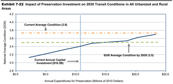
| Average Annual Investment (Billions of 2010 Dollars) Total Capital Outlay | Average Annual Percent Change vs. 2010 | Average Transit Conditions in 2030 Asset Categories | Notes | |||||
|---|---|---|---|---|---|---|---|---|
| Guideway | Facilities | Systems | Stations | Vehicles | All Transit Assets | |||
| $23.3 | 7.5% | 3.68 | 3.80 | 3.80 | 3.78 | 3.37 | 3.70 | Unconstrained, Replace at 3.00 |
| $20.2 | 6.3% | 3.65 | 3.43 | 3.70 | 3.76 | 3.33 | 3.62 | Unconstrained, Replace at 2.75 |
| $18.5 | 5.5% | 3.58 | 3.06 | 3.59 | 3.74 | 3.31 | 3.54 | SGR (Unconstrained, Replace at 2.50) |
| $12.7 | 2.0% | 3.45 | 2.85 | 3.55 | 3.74 | 3.36 | 3.48 | Maintain Current Backlog |
| $10.3 | 0.0% | 3.31 | 2.77 | 3.40 | 3.69 | 3.37 | 3.39 | 2010 Capital Expenditures |
| $8.6 | -1.9% | 3.26 | 2.73 | 3.30 | 3.67 | 3.27 | 3.34 | |
| $6.8 | -4.4% | 3.22 | 2.73 | 3.19 | 3.66 | 3.04 | 3.28 | |
| $4.4 | -9.9% | 3.21 | 2.70 | 3.08 | 3.64 | 2.65 | 3.20 | |
| $2.2 | -22.2% | 3.17 | 2.70 | 2.96 | 3.63 | 2.35 | 3.13 | |
Note that this preservation analysis is intended to consider reinvestment needs only for existing transit assets (as of 2010), not for expansion assets to be added to the existing capital stock in future years.
The table portion of Exhibit 7-22 presents the same investment and average condition information as in the chart. This table also presents the impact of reinvestment on asset conditions for five key transit asset categories (i.e., guideway and track, facilities, systems, stations, and vehicles) as well as the average annual percent change in constant dollar funding from 2010 levels to achieve each projected condition level.
Further review of Exhibit 7-22 reveals several observations. First, note that none of the selected reinvestment rates presented (including the current level of reinvestment, which was $10.3 billion in 2010) is sufficient to maintain aggregate conditions at or near the current national average condition rating of 3.8. Even the highest reinvestment rate presented here of $23.3 billion annually (replacement at condition rating 3.0), which represents a fairly aggressive reinvestment rate, is not quite sufficient to maintain aggregate conditions at current levels. A primary factor driving this result is the ongoing expansion investment in new rail systems over the past several decades, which has tended to maintain or even increase the average condition rating of assets nationwide (despite the ongoing deterioration of older assets), but has also resulted in an average condition rating that is not sustainable in the long term (i.e., without including the influence of further expansion investments or replacing assets at an unreasonably early age). Second, note that reinvestment at roughly $18.5 billion annually is required to attain a condition of SGR by 2030 and that this level of reinvestment is estimated to yield an average condition value of roughly 3.5 by 2030. Given the definition of the SGR benchmark (described in more detail in Chapter 8), which seeks to eliminate the existing investment backlog and then address all subsequent rehabilitation and replacement activities “on time” thereafter, the 3.5 value could be considered representative of the expected long-term average condition of a well-maintained and financially unconstrained national transit system. Hence, an average condition rating of roughly 3.5 represents a more reasonable long-term condition target for existing transit infrastructure than the current aggregate rating of 3.8.
A final observation is that a significant level of reinvestment is required to alter the estimated 2030 average condition measure by a point or more. This result is also driven in part by a large proportion of transit assets with expected useful lives of up to 80 years or more that will not require significant reinvestment over the 20-year period of this analysis (regardless of the level of reinvestment). These assets tend to contribute a high weighting in the average condition measure, making the measure somewhat insensitive to the rate of reinvestment (note that a high proportion of reinvestment activity is focused on the replacement of those assets with relatively shorter useful lives, such as vehicles).
Impact of Expansion Investments on Transit Ridership
While capital spending on preservation primarily benefits the physical condition of existing transit assets, expansion investments are typically undertaken to expand the asset base to accommodate projected growth in ridership and potentially to improve service performance for existing transit system users.
Exhibit 7-23 shows the relationship between aggregated annual capital spending by all levels of government on expansion investments and the additional number of annual passenger boardings that transit systems would be able to support by 2030. More precisely, this chart presents the level of expansion investment required to ensure that transit vehicle occupancy rates are maintained at current levels over the next two decades for a broad range of the potential rates of growth in transit passenger miles traveled (PMT). As the upward sloping curve of the chart indicates, higher levels of investment are required to support greater numbers of additional riders at a constant level of service. If investment levels are insufficient to fully support the projected growth in ridership, then vehicle occupancy rates will tend to increase, leading to increased crowding on high-utilization systems and potentially leading to increased dwell times at stops, reduced average operating speeds, and increased rates of vehicle wear. Conversely, if the rate of transit capacity expansion exceeds the actual rate of ridership growth, then occupancy rates will tend to decline and service performance would likely also improve.
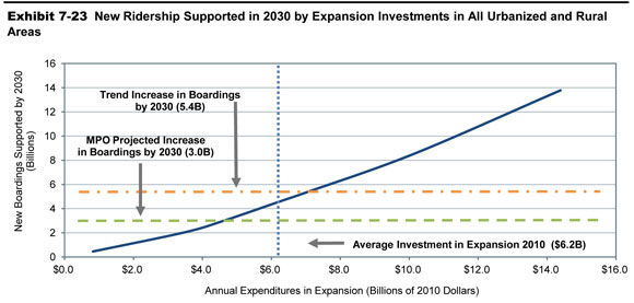
| Average Annual Investment (Billions of 2010 Dollars) | Average Annual Percent Change vs. 2010 | Total New Boardings by 2030 | Funding Level Description | |
|---|---|---|---|---|
| New Riders Supported (Billions of Annual Boardings) | Average Annual Growth in Boardings* | |||
| $14.4 | 7.7% | 13.8 | 4.3% | |
| $10.2 | 4.6% | 8.5 | 3.0% | |
| $7.1 | 1.3% | 5.4 | 2.1% | Trend Growth in PMT (1995 to 2010) |
| $6.2 | 0.0% | 4.6 | 1.8% | 2010 Capital Expenditures (Maintain Current Spending) |
| $4.6 | -3.5% | 3.0 | 1.3% | MPO Projected Increase in PMT |
| $3.5 | -6.3% | 2.0 | 0.9% | |
| $0.8 | -36.0% | 0.4 | 0.2% | |
The findings presented in Exhibit 7-23 suggest the following trends. First, the recent rate of investment in asset expansion ($6.2 billion in 2010) could support roughly 4.6 billion additional boardings by 2030 (approximately a 1.8 percent annual growth in ridership). This amount is greater than that required to support the level of growth projected by the Nation’s MPOs (roughly 1.3 percent when adjusted to exclude expansion investments that do not pass TERM’s benefit-cost test). As discussed in further detail in Chapter 9, MPO projections of transit growth (which are financially constrained) have typically fallen well short of actual growth in recent years. Assuming that the actual rate of ridership growth is close to the trend rate of growth for the last 15 years, then an average of $7.1 billion in annual transit capital expansion investment would be required over the next 20 years to support an additional 5.4 billion annual boardings (again after excluding expansion investments that do not pass TERM’s benefit-cost test). Hence, while the existing levels of transit capital expansion investment may be sufficient to maintain current service performance (i.e., vehicle occupancy rates) if ridership growth is relatively low, this level of investment is roughly two-thirds that required to support a level of ridership growth consistent with that experienced over the most recent 15-year period.
Impacts of Urbanized Area Investments Modeled by TERM
The remainder of this chapter focuses on how different levels of annual capital investment in the U.S. transit infrastructure affect urbanized areas with dissimilar transit investment needs. Specifically, this section explores the impact of capital expenditures by transit agencies sorted into two distinct UZA groupings: (1) the urbanized areas with populations greater than 1 million and (2) all other urbanized and rural areas with existing transit services.
Urbanized Areas Over 1 Million in Population
The Nation’s largest urbanized areas own and operate the majority of the Nation’s existing transit assets. These urbanized areas also typically have the highest levels of investment in older rail assets.
In 2010, transit agencies operating in urbanized areas with populations greater than 1 million expended $14.4 billion on capital projects, consisting of $9.0 billion on preservation investments intended to rehabilitate or replace existing assets, and $5.4 billion on expansion investments designed to increase service capacity. The following is a discussion of the transit asset preservation and expansion needs of these urbanized areas with populations greater than 1 million.
Preservation Investments
Exhibit 7-24 shows the estimated impact of varying levels of preservation investments on the future condition of existing transit assets located in urbanized areas with populations greater than 1 million. As with the earlier chart covering the entire industry, this chart clearly indicates that due to significant recent investments in long-lived expansion assets the current average condition rating for transit assets located in the largest urbanized areas is not sustainable in the long term without replacing assets on a fairly aggressive schedule (i.e., replacement at or before condition rating 3.0). At the same time, the 2010 level of reinvestment ($9.0 billion) is less than that required to attain a state of good repair ($16.0 billion), with the latter supporting a more sustainable long-term average condition rating of roughly 3.6.
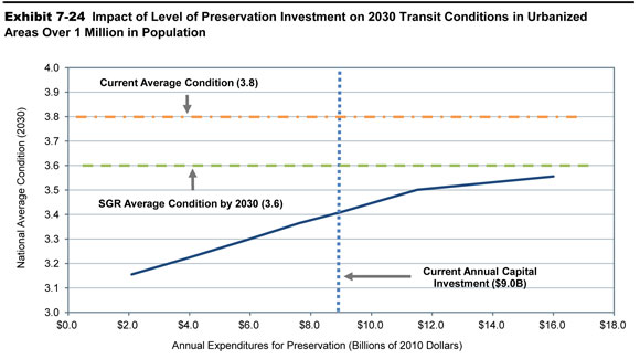
| Average Annual Investment (Billions of 2010 Dollars) Total Capital Outlay | Average Annual Percent Change vs. 2010 | Average Transit Conditions in 2030 Asset Categories | Notes | |||||
|---|---|---|---|---|---|---|---|---|
| Guideway | Facilities | Systems | Stations | Vehicles | All Transit Assets | |||
| $16.0 | 5.4% | 3.54 | 3.13 | 3.59 | 3.74 | 3.31 | 3.56 | SGR (Unconstrained Condition, Replace at 2.50) |
| $11.5 | 2.4% | 3.42 | 2.87 | 3.55 | 3.74 | 3.38 | 3.50 | Maintain Current Backlog |
| $9.0 | 0.0% | 3.30 | 2.75 | 3.41 | 3.69 | 3.37 | 3.41 | 2010 Capital Expenditures (Maintain Current Spending) |
| $7.6 | -1.7% | 3.25 | 2.70 | 3.30 | 3.67 | 3.28 | 3.36 | Reduce 2.5 Percent |
| $6.0 | -4.3% | 3.21 | 2.69 | 3.20 | 3.66 | 3.03 | 3.30 | Reduce 5 Percent |
| $4.0 | -9.4% | 3.19 | 2.65 | 3.09 | 3.64 | 2.68 | 3.22 | Reduce 10 Percent |
| $2.1 | -20.2% | 3.15 | 2.65 | 2.96 | 3.63 | 2.41 | 3.15 | Reduce 20 Percent |
As shown in Exhibit 7-25, the 2010 level of capital reinvestment of $9.0 billion for the largest urbanized areas is insufficient to keep pace with ongoing rehabilitation and replacement needs and, if maintained over the next 20 years, would result in a larger SGR backlog of roughly $120.4 billion by 2030 compared with the current $73.8 billion backlog. In contrast, increasing the rate of reinvestment to an annual average of roughly $16.0 billion will completely eliminate the entire backlog by 2030. The annual level of reinvestment would need to be increased to roughly $11.5 billion to maintain the backlog at roughly its current size.
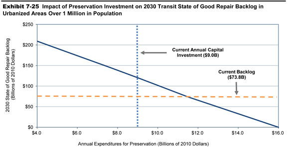
| Average Annual Investment (Billions of 2010 Dollars) | Average Annual Percent Change vs. 2010 |
Replacement Condition |
Average Condition Rating in 2030 |
Backlog in 2030 (Billions of 2010 Dollars) |
Funding Level Description |
|---|---|---|---|---|---|
| $16.0 | 5.4% | 2.50 | 3.56 | $0.0 | SGR (Unconstrained, Replace at 2.50) |
| $11.5 | 2.4% | 2.50 | 3.50 | $73.8 | Current Backlog |
| $9.0 | 0.0% | 2.50 | 3.41 | $120.4 | 2010 Capital Expenditures |
| $7.6 | -1.7% | 2.50 | 3.36 | $145.7 | |
| $6.0 | -4.3% | 2.50 | 3.30 | $173.9 | |
| $4.0 | -9.4% | 2.50 | 3.22 | $209.2 | |
Expansion Investments
Although urbanized areas with populations greater than 1 million tend to be cities with slower rates of increase in population and transit ridership (e.g., Boston, Philadelphia, and Chicago), this group also includes urbanized areas expected to experience relatively high rates of growth in transit boardings and PMT over the next two decades, including Los Angeles, Atlanta, and Seattle. Given the high numbers of existing riders and transit capacity in these higher-growth large urbanized areas, they will require significant increases in expansion investments to maintain current service performance during this time period.
Exhibit 7-26 presents estimates of the level of expansion investment required to support varying levels of growth in transit demand while maintaining current performance levels (as measured by vehicle capacity utilization) for these large urbanized areas. Note that the 2010 level of investment for these urbanized areas ($5.4 billion) was more than that required to support the rate of increase in transit demand as projected by the Nation’s MPOs (low growth) but well short of that required to support a rate of growth comparable to the trend rate of increase as experienced in recent years.
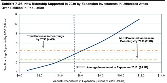
| Average Annual Investment (Billions of 2010 Dollars) | Average Annual Percent Change vs. 2010 | Total New Boardings by 2030 | Funding Level Description | |
|---|---|---|---|---|
| New Riders Supported (Billions of Annual Boardings) | Average Annual Growth in Boardings* | |||
| $11.8 | 7.3% | 11.0 | 4.0% | |
| $8.6 | 4.5% | 6.9 | 2.8% | |
| $6.1 | 1.3% | 4.4 | 2.0% | Trend Growth in PMT (1995 to 2010) |
| $5.4 | 0.0% | 3.7 | 1.7% | Maintain Spending (2010) |
| $4.1 | -2.8% | 2.5 | 1.2% | MPO Projected Growth |
| $3.2 | -5.6% | 1.7 | 0.8% | |
| $0.8 | -31.8% | 0.4 | 0.2% | |
Other Urbanized and Rural Areas
The following analysis considers the combined preservation and expansion needs of urbanized areas under 1 million in population and those of all rural areas with existing transit service. This diverse group therefore includes a large number of mid- and small-sized urbanized and rural transit operators offering only bus and/or paratransit services.
In 2010, transit agencies operating outside of the largest urbanized areas expended $2.2 billion on capital projects, consisting of $1.3 billion on preservation investments intended to rehabilitate or replace existing assets, and $0.9 billion on expansion investments designed to increase service capacity. The following is a discussion of the transit asset preservation and expansion needs of transit agencies in these areas.
Preservation Investments
Exhibit 7-27 shows the estimated impact of varying levels of preservation investments on the future condition of existing transit assets located in urbanized areas with populations less than 1 million and in rural areas. As with the earlier analyses for the largest urbanized areas, this chart also indicates that the current average condition rating for transit assets in these smaller urbanized and rural areas is not sustainable in the long term without replacing assets on a fairly aggressive schedule (i.e., replacement at or before condition rating 3.0). At the same time, the 2010 level of reinvestment ($1.3 billion) is significantly less than that required to attain an SGR ($2.5 billion), with the latter supporting a more sustainable long-term average condition rating of roughly 3.4.
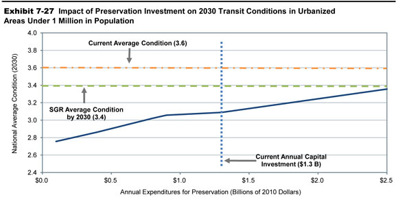
| Average Annual Investment (Billions of 2010 Dollars) Total Capital Outlay | Average Annual Percent Change vs. 2010 | Average Transit Conditions in 2030 Asset Categories | Notes | |||||
|---|---|---|---|---|---|---|---|---|
| Guideway | Facilities | Systems | Stations | Vehicles | All Transit Assets | |||
| $2.5 | 7.5% | 4.45 | 2.93 | 3.73 | 3.87 | 3.30 | 3.36 | SGR (Unconstrained, Replace at 2.5) |
| $1.3 | 0.0% | 3.57 | 2.79 | 3.11 | 3.75 | 3.32 | 3.09 | 2010 Capital Expenditures (Maintain Current Spending) |
| $0.90 | -2.1% | 3.57 | 2.78 | 3.05 | 3.51 | 3.23 | 3.06 | Reduce 2.5 Percent |
| $0.8 | -3.3% | 3.57 | 2.78 | 3.03 | 3.41 | 3.09 | 3.02 | Reduce 5 Percent |
| $0.4 | -12.2% | 3.57 | 2.78 | 2.99 | 3.38 | 2.37 | 2.86 | Reduce 10 Percent |
| $0.1 | -52.1% | 3.57 | 2.78 | 2.98 | 3.35 | 1.88 | 2.76 | Reduce 20 Percent |
As shown in Exhibit 7-28, the 2010 level of capital reinvestment of $1.3 billion for rural areas and smaller urbanized areas is insufficient to keep pace with ongoing rehabilitation and replacement needs. If maintained over the next 20 years, this rate of investment would result in a larger SGR backlog of roughly $21.3 billion by 2030, as compared with the current backlog of $6.8 billion for this group. In contrast, increasing the rate of reinvestment to an annual average of roughly $2.5 billion will completely eliminate the entire backlog by 2030. The annual level of reinvestment would need to be increased to roughly $1.8 billion annually to maintain the backlog at roughly its current size.
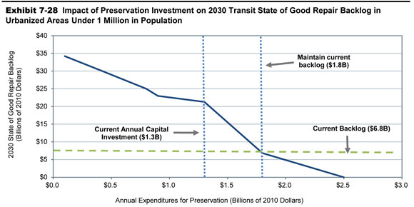
| Average Annual Investment (Billions of 2010 Dollars) | Average Annual Percent Change vs. 2010 |
Replacement Condition |
Average Condition Rating in 2030 |
Backlog in 2030 (Billions of 2010 Dollars) |
Funding Level Description |
|---|---|---|---|---|---|
| $2.5 | 7.5% | 2.50 | 3.36 | $0.0 | SGR (Unconstrained, Replace at 2.50) |
| $1.8 | 4.7% | 2.50 | 3.17 | $6.8 | Current Backlog |
| $1.3 | 0.0% | 2.50 | 3.09 | $21.3 | 2010 Capital Expenditures |
| $0.9 | -2.1% | 2.50 | 3.06 | $23.0 | |
| $0.8 | -3.3% | 2.50 | 3.02 | $25.0 | |
| $0.4 | -12.2% | 2.00 | 2.86 | $30.3 | |
| $0.1 | -52.2% | 2.50 | 2.76 | $34.2 | |
Expansion Investments
While the urbanized and rural areas in this group represent a smaller number of riders and a smaller existing transit asset base, these areas are also expected to have a higher projected rate of increase in transit ridership.
Exhibit 7-29 presents estimates of the level of expansion investment required to support varying levels of growth in transit demand while maintaining current performance levels (as measured by transit passenger miles per peak vehicle) for the smaller urbanized and all rural areas. Note that the 2010 level of investment for these areas ($0.9 billion) was the same as that required to support the rate of increase in transit demand as projected by the Nation’s MPOs and slightly less than the trend rate of increase as experienced over the last several years. Such investments should yield improvements in transit performance in these urbanized areas and also help promote transit-led urban development in urbanized areas subject to above average rates of population and transit growth.
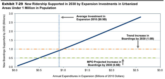
| Average Annual Investment (Billions of 2010 Dollars) | Average Annual Percent Change vs. 2010 | Total New Boardings by 2030 | Funding Level Description | |
|---|---|---|---|---|
| New Riders Supported (Billions of Annual Boardings) | Average Annual Growth in Boardings* | |||
| $2.6 | 9.9% | 2.8 | 6.4% | |
| $1.5 | 5.1% | 1.6 | 4.5% | |
| $1.0 | 1.4% | 1.0 | 3.2% | Trend Growth in PMT (1995 to 2010) |
| $0.9 | 0.0% | 0.9 | 2.8% | Maintain Spending (2010) |
| $0.5 | -7.3% | 0.5 | 1.6% | MPO Projected Growth |
| $0.3 | -11.6% | 0.3 | 1.3% | |
| $0.1 | -68.0% | 0.1 | 0.3% | |