
The differences shown in the previous sections do not indicate which version is performing better with respect to measured data. In order to determine how well a given version performs, comparisons of measured and modeled data are required. Because measured data were not available for the CTS sites, only the sites described in Section 2 are included in these comparisons.
In the following sections, four sets of comparisons to measured data are performed using modeled results from: 1) TNM 2.5 with Average pavement, 2) TNM 3.0 with Average pavement, 3) TNM 2.5 with specific pavements, and 4) TNM 3.0 with specific pavements10. (Note that since the goal of this section is to evaluate performance and not to identify root causes, TNM 2.6 analyses is omitted.) Although other factors are confounded with pavement type, comparing predicted and measured data modeled with specific pavement type can provide additional insight by accounting for one known deviation between sites as modeled and actual measurements. Assuming that study sites are well represented by the REMELs database, one would expect sites that had PCC roadways to be under-predicted (at least near the source) and sites that had DGAC or OGAC to be over-predicted when Average pavement is used.
Section 7.1 compares the performance of TNM 2.5 and TNM 3.0 relative to measured data for all data analyzed. However, in order to determine if TNM 3.0 is performing better or worse for a specific type of site, a more detailed analysis is required. To this end, the performances of TNM 2.5 and TNM 3.0 relative to measured data were also compared, for sites with acoustically hard or soft ground, for sites with or without a barrier, and receivers at near, medium and far distances, and on a site-by-site basis. The results of these comparisons are summarized in Sections 7.2 through 7.5.
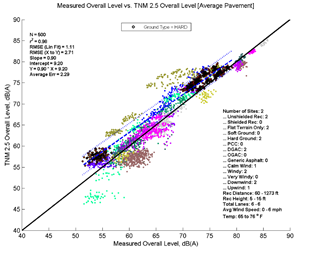
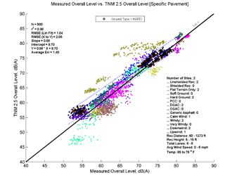
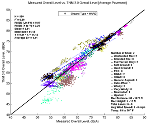
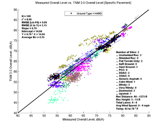
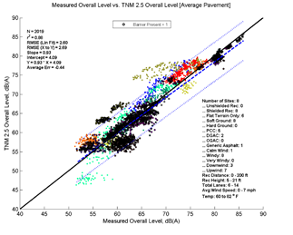
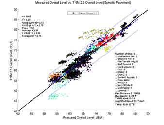
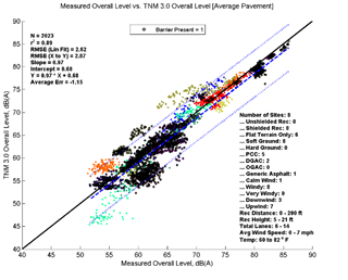
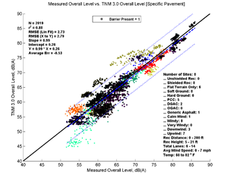
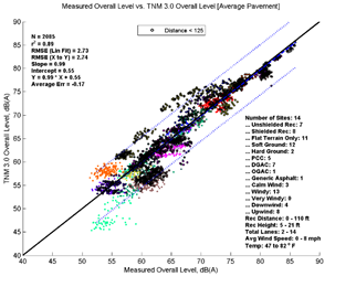
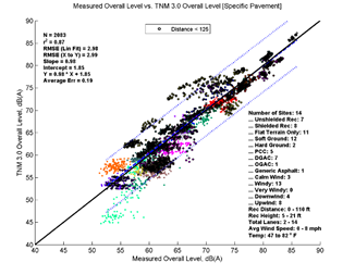
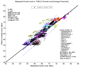
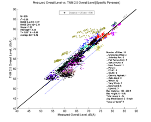
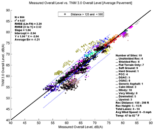
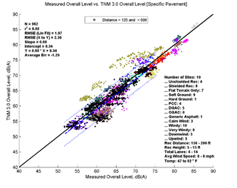
Figure 13 depicts the performance of TNM 2.5 and TNM 3.0 relative to measured data for all data analyzed. The formatting is similar to Figure 3, but the levels on the x-axis correspond to measured data instead of a second set of modeled data. The top left pane of Figure 13 shows TNM 2.5 with Average pavement compared to measured data, while the bottom left pane shows TNM 3.0 modeled with Average pavement compared to measured data. The right panes show TNM 2.5 and TNM 3.0 comparisons modeled with specific pavements. As in Figure 3, the colored data points (each site is presented in a different color) represent individual 5-minute model computations; the dashed line shows the first-order linear regression between the two datasets; the dotted lines indicate the 95-percent prediction interval for any new samples; and the solid black line indicates where all results would fall if the model predicted the measured results with perfect agreement. Note that in the upper left hand corner of graph several statistical parameters are presented: the number of samples, the coefficient of determination (r2), the root mean squared error (RMSE), the regression slope and intercept, the regression equation, and the average error. In the lower right-hand corner, a metadata summary is provided covering the number of sites, the presence of a barrier, receiver distances and heights, number of roadway lanes, pavement type, and temperature and wind conditions included in the analysis.
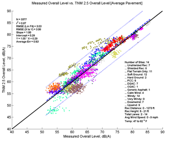
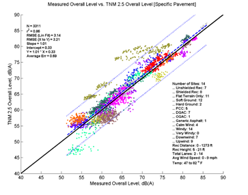
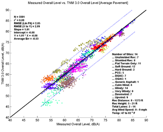
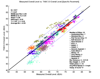
Figure 13, shows that TNM 2.5 (top two graphics) on average over predicts the measured data while TNM 3.0 (bottom two graphics) under predicts the measured data. This trend is consistent over the range of measured sound levels; the offset between the solid black line and dashed regression line is nearly constant. Modeling with specific pavement types does not change the overall picture greatly; the same general trends are visible in both sets of results. These results are very consistent with the comparisons in Section 5, with the main difference being increased variation due the measured data.
In order to better compare and quantitatively describe model performance, the statistical parameters presented in the upper left-hand corner of the graphics are replicated in Table 6 below. When comparing measured to modeled data, the average error statistic provides an indication of the overall average difference between measured and modeled results. Modeled with average pavement, TNM 2.5, on average over predicts these data by 0.53 dB, while TNM 3.0 under predicts these data by 0.53 dB. Modeled with specific pavements, the average error is shifted upward to 0.69 for TNM 2.5 and -0.36 for TNM 3.0; a result of modeling 5 of the 14 sites with PCC pavement. Because PCC typically has much higher sound pressure levels than Average pavement, while DGAC has only slightly lower sound pressure levels than Average pavement for the same traffic, one would expect an upward shift in these results modeled with specific pavements.
The slope for these regressions can indicate if the error changes with a change in the x-axis values (sound level). In all four cases, the slope coefficient is equal to or nearly equal to 1.0, indicating no change in model performance over the range of sound levels.
TNM 3.0 achieves a slightly better r2 values than TNM 2.5; however, the difference is quite small (r2 of 0.88 compared to 0.87 for Average pavement). TNM 3.0 has an RMSE of 2.85 while TNM 2.5 has an RMSE of 3.03. This indicates that the difference between TNM 3.0 predictions and measured data are slightly less random than the difference between TNM 2.5 predictions and measured data.
| Average Measured vs. TNM 2.5 | Specific Measured vs. TNM 2.5 | Average Measured vs. TNM 3.0 | Specific Measured vs. TNM 3.0 | |
|---|---|---|---|---|
| N | 3377 | 3311 | 3381 | 3377 |
| r2 | 0.87 | 0.86 | 0.88 | 0.87 |
| RMSE (Lin Fit) | 3.03 | 3.14 | 2.85 | 2.99 |
| RMSE (X to Y) | 3.08 | 3.21 | 2.89 | 3.01 |
| Slope | 1.00 | 1.01 | 1.01 | 1 |
| Intercept | 0.29 | 0.33 | -0.88 | -0.59 |
| Average Err | 0.53 | 0.69 | -0.53 | -0.36 |
| Slope 95% CI | 0.99, 1.02 | 0.99, 1.02 | 0.99, 1.02 | 0.99, 1.02 |
| Intercept 95% CI | -0.58, 1.17 | -0.58, 1.24 | -1.70, -0.06 | -1.45, 0.27 |
| Avg Err 95% CI | 0.43, 0.64 | 0.58, 0.80 | -0.63, -0.43 | -0.46, -0.26 |
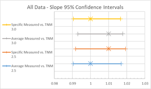
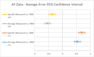
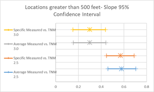
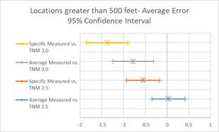
To further visualize these summary statistics, graphics in Figure 14 depict the 95% confidence intervals (CI) for the estimated slope and average error parameters. These graphics can show if differences between these values are statistically significant. Overlapping lines would indicate that the values are statistically similar, while non-overlapping lines would indicate that these values are not statistically similar. In Figure 15, the slopes of all four regression lines are statistically similar, while the average errors between 2.5 and 3.0 are not.
To determine if TNM 3.0 is performing better or worse for a specific type of site, a more detailed analysis may be required. To this end, the performances of TNM 2.5 and TNM 3.0 relative to measured data were compared for sub-sets of the data including:
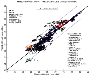
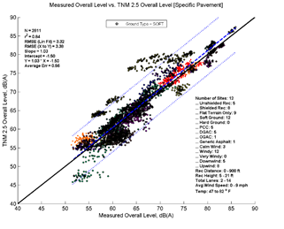
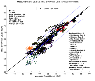
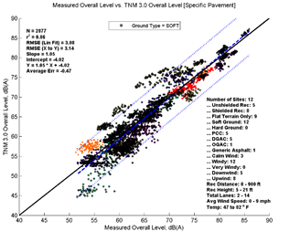
Figure 15, Table 7 and Figure 16 show the agreement between predicted and measured results for all cases where acoustically soft ground was the primary ground type between source and receiver. The soft ground data are represented by the black data points; all other data (shown in the graph but not included in the regression) are represented in the background by colored data points. When modeled with Average pavement, TNM 2.5 has good prediction results for all statistics computed and the trend line almost directly coincides with the line representing a one-to-one relationship. The average difference is just 0.23 dB. Results show slightly less agreement when modeled with specific pavements; TNM 2.5 over predicts by 0.56 dB (average error) and the slope of the trend line is now greater than one, influenced by the upward shift in predicted levels for sites modeled with PCC pavement.
TNM 3.0 on average under predicts soft ground by 0.81 dB with Average pavement and by 0.47 dB with specific pavement. Again, the slope of the trend line for specific pavements is influenced by the upward shift in predictions due to sites modeled with PCC pavement.\
| Average Measured vs. TNM 2.5 | Specific Measured vs. TNM 2.5 | Average Measured vs. TNM 3.0 | Specific Measured vs. TNM 3.0 | |
|---|---|---|---|---|
| N | 2877 | 2811 | 2881 | 2877 |
| r2 | 0.85 | 0.84 | 0.88 | 0.86 |
| RMSE (Lin Fit) | 3.13 | 3.32 | 2.86 | 3.08 |
| RMSE (X to Y) | 3.14 | 3.38 | 2.99 | 3.14 |
| Slope | 1.01 | 1.03 | 1.04 | 1.05 |
| Intercept | -0.42 | -1.5 | -3.36 | -4.02 |
| Average Err | 0.23 | 0.56 | -0.81 | -0.47 |
| Slope 95% CI | 0.99, 1.03 | 1.01, 1.05 | 1.02, 1.05 | 1.04, 1.07 |
| Intercept 95% CI | -1.45, 0.60 | -2.60, -0.40 | -4.30, -2.43 | -5.03, -3.01 |
| Avg Err 95% CI | 0.11, 0.34 | 0.44, 0.67 | -0.92, -0.71 | -0.58, -0.35 |
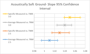
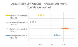
Figure 17, Table 8, and Figure 18 show the agreement between predicted and measured results for TNM 2.5 and 3.0 for all cases where hard ground was the primary ground type between source and receiver. As these trend lines are based on only two sites, conclusions drawn from these regressions could be amended in the presence of more data.
TNM 3.0 performs better for these hard ground cases, having smaller average errors and RMSE. On average both versions over predict noise levels, with over-predictions greater at farther distances11. As expected, the over-prediction is slightly less when modeled with specific pavement, which is DGAC for both sites. However, while TNM 2.5 also over-predicts noise levels at near distances, TNM 3.0 has smaller average errors and RMSE at near distances and actually slightly under predicts when modeled with specific pavement. When modeled with specific pavement, the average error for TNM 3.0 is lowest, as the over-prediction at far distances and under-prediction at near distances result in an average of nearly zero. (This does not inherently represent better performance, merely a preferable alignment of errors.)
| Average Measured vs. TNM 2.5 | Specific Measured vs. TNM 2.5 | Average Measured vs. TNM 3.0 | Specific Measured vs. TNM 3.0 | |
|---|---|---|---|---|
| N | 500 | 500 | 500 | 500 |
| r2 | 0.98 | 0.98 | 0.99 | 0.98 |
| RMSE (Lin Fit) | 1.11 | 1.04 | 0.87 | 0.89 |
| RMSE (X to Y) | 2.71 | 2.06 | 2.26 | 2.15 |
| Slope | 0.9 | 0.88 | 0.81 | 0.79 |
| Intercept | 9.2 | 9.7 | 14.45 | 14.84 |
| Average Err | 2.29 | 1.4 | 1.11 | 0.25 |
| Slope 95% CI | 0.89, 0.91 | 0.87, 0.89 | 0.80, 0.81 | 0.78, 0.80 |
| Intercept 95% CI | 8.46, 9.94 | 9.01, 10.40 | 13.87, 15.03 | 14.24, 15.43 |
| Avg Err 95% CI | 2.17, 2.42 | 1.26 , 1.53 | 0.93, 1.28 | 0.06, 0.44 |
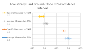
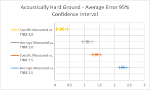
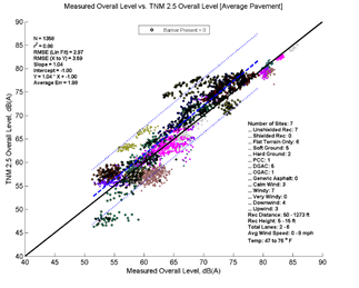
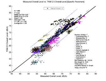
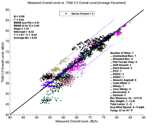
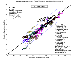
Figure 19, Table 9, and Figure 20 show the agreement between predicted and measured results for TNM 2.5 and 3.0 for all open sites where no barrier is between source and receiver. On average, TNM 3.0 has nearly perfect agreement when modeled with Average pavement, while there is a slight under-prediction when modeled with specific pavements (most of the sites have DGAC as the specific pavement).
| Average Measured vs. TNM 2.5 | Specific Measured vs. TNM 2.5 | Average Measured vs. TNM 3.0 | Specific Measured vs. TNM 3.0 | |
|---|---|---|---|---|
| N | 1358 | 1358 | 1358 | 1358 |
| r2 | 0.88 | 0.84 | 0.88 | 0.85 |
| RMSE (Lin Fit) | 2.97 | 3.47 | 2.91 | 3.32 |
| RMSE (X to Y) | 3.59 | 3.78 | 2.93 | 3.32 |
| Slope | 1.04 | 1.05 | 1.01 | 1.02 |
| Intercept | -1 | -1.62 | -0.42 | -1.15 |
| Average Err | 1.98 | 1.46 | 0.4 | -0.11 |
| Slope 95% CI | 1.024, 1.07 | 1.02, 1.07 | 0.99, 1.03 | 0.99, 1.04 |
| Intercept 95% CI | -2.39, 0.38 | -3.25, 0.00 | -1.78, 0.94 | -2.70, 0.41 |
| Avg Err 95% CI | 1.83, 2.14 | 1.28, 1.65 | 0.24, 0.55 | -0.29, 0.06 |
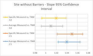
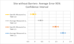
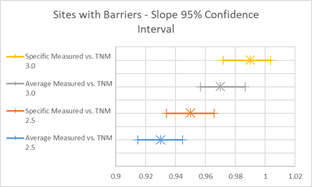
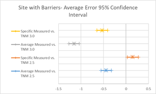
Figure 21, Table 10 and Figure 22 show the agreement between predicted and measured results for TNM 2.5 and 3.0 for all cases where there is a barrier between source and receiver. Both versions of TNM under predict the "with Barrier" cases on average. TNM 2.5 under predicts less than TNM 3.0 (average error -0.44 vs. -1.15). The under-prediction decreases with specific pavement, as most sites in this group had PCC pavements.
| Average Measured vs. TNM 2.5 | Specific Measured vs. TNM 2.5 | Average Measured vs. TNM 3.0 | Specific Measured vs. TNM 3.0 | |
|---|---|---|---|---|
| N | 2019 | 1953 | 2023 | 2019 |
| r2 | 0.88 | 0.87 | 0.89 | 0.88 |
| RMSE (Lin Fit) | 2.6 | 2.72 | 2.62 | 2.73 |
| RMSE (X to Y) | 2.69 | 2.75 | 2.87 | 2.79 |
| Slope | 0.93 | 0.95 | 0.97 | 0.99 |
| Intercept | 4.09 | 3.38 | 0.68 | 0.26 |
| Average Err | -0.44 | 0.15 | -1.15 | -0.53 |
| Slope 95% CI | 0.91, 0.94 | 0.93, 0.97 | 0.96, 0.99 | 0.97, 1.00 |
| Intercept 95% CI | 3.12, 5.06 | 2.34, 4.42 | -0.30, 1.66 | -0.76, 1.29 |
| Avg Err 95% CI | -0.56, -0.33 | 0.03, 0.27 | -1.27, -1.04 | -0.65, -0.41 |
Distance effects are especially difficult to analyze in the aggregate because all possible confounding factors, including hard and soft ground types and barrier presence, tend to show up in each distance category. Therefore, interactions between distance and ground type, barrier presence, and pavement type may be present at all distances. Even so, it is still useful to consider how each model is performing at various distances.
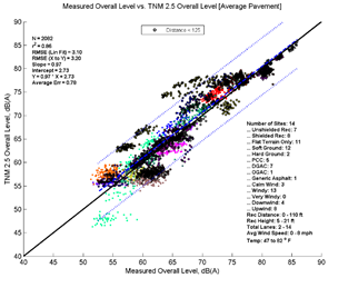
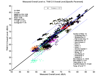
Figure 23, Table 11, and Figure 24 show the agreement between predicted and measured results for TNM 2.5 and 3.0 for distances less than 125 feet between source and receiver. Here TNM 2.5 tends to slightly over predict levels (average error = 0.78 dB) while TNM 3.0 tends to slightly under predict levels (average error = -0.17 dB). TNM 3.0's RMSE is also about 0.5 dB smaller than TNM 2.5. Otherwise, most descriptors are very similar between the two versions for this distance.
| Average Measured vs. TNM 2.5 | Specific Measured vs. TNM 2.5 | Average Measured vs. TNM 3.0 | Specific Measured vs. TNM 3.0 | |
|---|---|---|---|---|
| N | 2082 | 2044 | 2085 | 2083 |
| r2 | 0.86 | 0.84 | 0.89 | 0.87 |
| RMSE (Lin Fit) | 3.1 | 3.35 | 2.73 | 2.98 |
| RMSE (X to Y) | 3.2 | 3.55 | 2.74 | 2.99 |
| Slope | 0.97 | 0.96 | 0.99 | 0.98 |
| Intercept | 2.73 | 3.74 | 0.55 | 1.85 |
| Average Err | 0.78 | 1.15 | -0.17 | 0.19 |
| Slope 95% CI | 0.95, 0.99 | 0.94, 0.98 | 0.97, 1.00 | 0.96, 0.99 |
| Intercept 95% CI | 1.58, 3.87 | 2.49, 4.99 | -0.46, 1.56 | 0.75, 2.95 |
| Avg Err 95% CI | 0.64, 0.91 | 1.01, 1.30 | -0.29, -0.06 | 0.06, 0.31 |
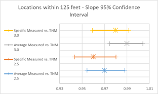
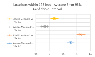
Figure 25, Table 12 and Figure 26 show the agreement between predicted and measured results for TNM 2.5 and 3.0 from 125 to 500 feet between source and receiver. TNM 2.5 on average over predicts slightly (0.18 dB) while TNM 3.0 under predicts by about 1.21 dB.
| Average Measured vs. TNM 2.5 | Specific Measured vs. TNM 2.5 | Average Measured vs. TNM 3.0 | Specific Measured vs. TNM 3.0 | |
|---|---|---|---|---|
| N | 963 | 935 | 964 | 962 |
| r2 | 0.85 | 0.88 | 0.87 | 0.88 |
| RMSE (Lin Fit) | 2.55 | 2.11 | 2.2 | 1.97 |
| RMSE (X to Y) | 2.6 | 2.11 | 2.52 | 2.3 |
| Slope | 1.09 | 1.03 | 1.04 | 0.98 |
| Intercept | -5.59 | -1.49 | -3.94 | 0.34 |
| Average Err | 0.18 | 0.12 | -1.21 | -1.2 |
| Slope 95% CI | 1.06, 1.12 | 1.00, 1.05 | 1.02, 1.07 | 0.95, 1.00 |
| Intercept 95% CI | -7.49, -3.70 | -3.07, 0.08 | -5.57, -2.30 | -1.12, 1.80 |
| Avg Err 95% CI | 0.02, 0.34 | -0.02, 0.25 | -1.35, -1.07 | -1.32, -1.07 |
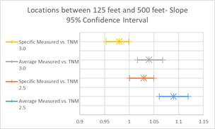
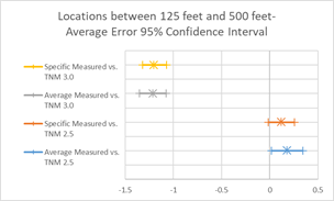
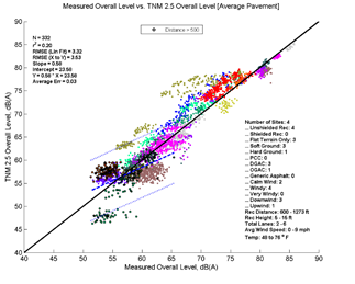
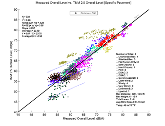
Figure 27, Table 13, and Figure 28 show the agreement between predicted and measured results for TNM 2.5 and 3.0 for distances greater than 500 feet between source and receiver. TNM 2.5 on average with measured results (average error = 0.03) while TNM 3.0 (Average pavement) under predicts by about 0.78 dB. It should be noted that, because the spread of measured data for this last distance range is short, many of the regression statistics (r2, slope, intercept) may be exaggerated.
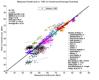
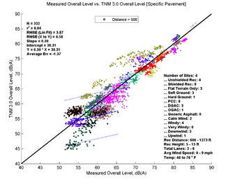
| Average Measured vs. TNM 2.5 | Specific Measured vs. TNM 2.5 | Average Measured vs. TNM 3.0 | Specific Measured vs. TNM 3.0 | |
|---|---|---|---|---|
| N | 332 | 332 | 332 | 332 |
| r2 | 0.2 | 0.2 | 0.05 | 0.04 |
| RMSE (Lin Fit) | 3.32 | 3.29 | 3.87 | 3.87 |
| RMSE (X to Y) | 3.53 | 3.56 | 4.44 | 4.58 |
| Slope | 0.58 | 0.57 | 0.3 | 0.3 |
| Intercept | 23.58 | 23.7 | 38.71 | 38.31 |
| Average Err | 0.03 | -0.55 | -0.78 | -1.37 |
| Slope 95% CI | 0.46, 0.70 | 0.45, 0.69 | 0.16, 0.44 | 0.15, 0.44 |
| Intercept 95% CI | 16.66, 30.50 | 16.84, 30.57 | 30.63, 46.79 | 30.24, 46.38 |
| Avg Err 95% CI | -0.35, 0.41 | -0.93, -0.18 | -1.25, -0.31 | -1.84, -0.90 |
Examining each site on its own is useful to see how well the predictions match for a specific set of conditions (compared to the aggregate groups discussed up to this point). Table 14 presents a summary of the average error statistics and site characteristics for TNM model runs for each site. In general, the trends for these individual sites will mirror trends for the groupings noted in the previous sections. For example, TNM 2.5 tends to over predict measured data while TNM 3.0 tends to under predict measured data; modeling with specific pavements increases overall levels when sites include PCC pavements; Graphics and model summary tables similar to those presented in previous sections are presented in Appendix H: Comparison of Modeled and Measured Results (Not Adjusted for Reference Microphone).
| Site ID | Site Type | Pavement | Average Error Statistic | ||||||||||
|---|---|---|---|---|---|---|---|---|---|---|---|---|---|
| Average Measured vs. TNM 2.5 | Specific Measured vs. TNM 2.5 | Average Measured vs. TNM 3.0 | Specific Measured vs. TNM 3.0 | ||||||||||
| Open area | Noise barrier | Soft ground | Hard ground | Mixed ground | Flat | With drop-off | Undulating | ||||||
| 01MA | X | X | X | DGAC | 3.55 | 2.51 | 1.49 | 0.5 | |||||
| 02MA | X | X | X | DGAC | 0.34 | -0.44 | -1.35 | -2.12 | |||||
| 03MA | X | X | X | DGAC | 0.27 | -0.42 | -1.97 | -2.6 | |||||
| 05CA | X | X | X | PCC | 0.37 | 1.58 | -0.12 | 1.26 | |||||
| 06CA | X | X | X | X | DGAC | 1.54 | 1.00 | 0.02 | -0.72 | ||||
| 08CA | X | X | X | PCC | 0.01 | 1.25 | -0.47 | 1.08 | |||||
| 09CA | X | X | X | X | PCC | -3.62 | -2.87 | -4.55 | -3.55 | ||||
| 10CA | X | X | X | X | PCC | 6.00 | 7.47 | 4.07 | 5.46 | ||||
| 11CA | X | X | X | DGAC | -0.65 | -1.44 | -0.92 | -1.84 | |||||
| 12CA | X | X | X | PCC | -0.76 | 0.48 | -1.21 | 0.22 | |||||
| 13CA | X | X | X | OGAC | -1.76 | -2.73 | -1.82 | -2.79 | |||||
| 14CA | X | X | X | DGAC | -0.22 | -0.22 | -0.7 | -1.51 | |||||
| 16MA | X | X | X | DGAC | 2.08 | 1.02 | 0 | -0.99 | |||||
| 17CT | X | X | X | DGAC | 2.64 | 2.00 | 2.91 | 2.27 | |||||
10 Here specific pavement refers to the pavement identified during the site scoping and is either DGAC, OGAC, or PCC.
11 Although other factors play a role, in general lower sound pressure levels indicate data collected far from the roadway and higher sound pressure levels indicate data collected nearer to the roadway. This interpretation is used whenever distance is not explicitly given.

