Previous Chapter « Table of Contents » Next Chapter
To provide a better understanding of the current state of traffic monitoring in recreational areas, background information is provided related to:
Recreational traffic is distinct with respect to the types of vehicles in the traffic stream and the corresponding average vehicle occupancy. In general, recreational traffic comprises a higher proportion of recreational vehicles (RVs), buses, and vehicles pulling trailers. Alternative transportation initiatives, such as the Paul S. Sarbanes Transit in the Parks Program, may increase the volume of buses in certain recreational areas. The average vehicle occupancy tends to be higher than that of commuter or local traffic.
Recreational trips can be either destination-focused or for leisure, where much of the drive time is considered to be recreation. Trip routing is directly influenced by its purpose. Recreational trips also have a high temporal variability (e.g., by time of day, day of week, season) depending upon the nature of recreational activities available. Unlike commuter or local traffic where the mean time between trips is both minimal and somewhat predictable, the mean time between recreational trips can range from several days to one week to one year or more. Recreational trips are discretionary, and as such, are readily influenced by factors such as weather, gas prices, etc.
The roadways that support recreational travel differ significantly from roads that are primarily commuter or industrial. Roadways that predominantly support recreational travel are generally of lower functional class, have constrained geometric design features, and may be paved, gravel, or native surfacing. Many are low or extremely low volume roads.
At the Federal level, primary agencies that are directly responsible planning and managing the preservation and use of recreational areas include:
These agencies differ in their underlying mission and priorities and the nature and extent of their jurisdictional land areas and associated roadway network.
The BLM administers a variety of programs for the management and conservation of resources on 256 million surface acres as well as 700 million subsurface mineral acres of land in the United States. These public lands comprise approximately 13% of the total land surface of the United States and more than 40% of all land managed by the Federal Government. Most of the public lands are located in the Western United States (including Alaska) and are characterized by grassland, forest, mountain, arctic tundra, and desert landscapes. The BLM manages the land's resources and uses including energy, minerals, timber, recreation, wild horse and burro herds, fish and wildlife habitat, wilderness areas, and archaeological, paleontological, and historical sites. 10
An estimated 600,000 miles of roadways service these public lands. Of these roads 90,000 miles are identified as "system routes" and are eligible for planning, maintenance, and funding. No formal process for managing or maintaining the remaining 510,000 miles of roadway presently exists. Visits to recreation sites on BLM lands and waters have significantly increased over the years from 51 million in 2001, to 57 million in 2008. 11
The USFWS is dedicated to the conservation, protection, and enhancement of the habitats of fish, wildlife, and plants. The agency is also responsible for implementing and enforcing some of the Nation's environmental laws, including the Endangered Species Act, Migratory Bird Treaty Act, Marine Mammal Protection Act, North American Wetlands Conservation Act, and Lacey Act.
The USFWS manages the 96 million acre, 548-unit, National Wildlife Refuge System. More than 4,900 miles of roadway currently service USFWS lands. Visits to recreation sites on USFWS lands and waters are expected to significantly increase from 41 million in 2008 to 51 million in 2015. The USFWS also operates 70 National Fish Hatcheries, which, in conjunction with Fish Health Centers and Fish Technology Centers, restore native aquatic populations, mitigate for fisheries lost as a result of Federal water projects, and support recreational fisheries throughout the United States. 12
The USDA-FS manages public lands in 155 national forests and 20 grasslands, encompassing 193 million acres. The USDA-FS is the largest forestry research organization in the world, and provides technical and financial assistance to State and private forestry agencies.
Access to USDA-FS lands is provided through a combination of public highways, local public roads, and classified USDA-FS roads within the National Forest System. An estimated 380,000 miles of classified USDA-FS roadways exist, with much of this roadway network established to support timber harvest and log removal. Approximately 66,000 miles of USDA-FS roadway is maintained to support passenger car traffic; the remaining roadway network supports only high-clearance vehicles. An estimated 1.7 million vehicles use these roads each day to visit national forests. 13
About 29,000 miles of State and local roads are designated as Forest Highways. As indicated in 23 U.S.C. 202, 203, and 204, the Forest Highways program, developed in cooperation with State and local agencies, provides safe and adequate transportation access to and through National Forest System (NFS) lands for visitors, recreationists, resource users, and others which is not met by other transportation programs. Forest highways assist rural and community economic development and promote tourism and travel.
The NPS manages a network of nearly 400 natural, cultural, and recreational sites across the Nation with the intent of preserving the sites for the enjoyment, education, and inspiration of current and future generations. The NPS also cooperates with partners to extend the benefits of resource conservation and outdoor recreation throughout the United States and the world. 14
Approximately 8,500 miles of roadway service NPS lands; 5,456 miles of which are paved. An estimated 90 percent of the road miles exist in just 10 percent of the parks. 15 The NPS roadway network also includes 1,736 bridges and 67 tunnels. Alternative transportation systems operate in 96 of the nearly 400 parks. The NPS routinely monitors the number of vehicles entering 297 parks along highways, parkways, and tour and access roads (paved and unpaved). Approximately 110 million vehicles or 218 million visitors enter the NPS lands for recreational purposes each year. An additional 218 million vehicles are estimated to access NPS lands for non-recreational purposes (e.g., NPS employees or contracted services, through traffic, etc.). 16
At the State level, DOTs collect traffic data to meet Federal reporting requirements and to support decision-making needs within the State. Each State DOT must comply with the reporting requirements of the Highway Performance Monitoring System (HPMS). These data - focused on traffic volumes for a subset of roadways in a State - are used to produce statewide estimates of total vehicle-miles traveled (VMT) and the subsequent apportionment of Federal- aid funds. Additional data collected to support State-level decision-making varies widely depending on each State DOT's traffic counting needs, priorities, budgets, geography, and organizational constraints.
Differences in the nature and extent of recreational activity in each State and its relationship to the roadway network exacerbate differences in recreational traffic monitoring. For example, recreational areas and activities are highly concentrated in Florida; as a result, a high proportion of the system and secondary roadways carry recreational trips. The State's traffic monitoring activities are designed to account for this. Comparatively, Colorado's system roadways also carry recreational trips but this segment of travelers is likely considered to be secondary when planning and designing traffic monitoring activities. In Wyoming, many of the major system routes currently monitored directly feed recreational areas in the State.
The Office of Federal Lands Highway (FLH) FHWA, under the U.S. Department of Transportation, provides funding for public roads and highways within federally owned lands and tribal lands that are not a State or local government responsibility. The FLH has close partnerships with State and local governments and works with numerous Federal land management agencies including the Bureau of Land Management, Fish and Wildlife Service, Forest Service, National Park Service, Bureau of Indian Affairs, Bureau of Reclamation, Surface Deployment and Distribution Command, and the U.S. Army Corps of Engineers.
The challenge of collecting recreational traffic data is also complicated by a lack of consistent guidance; existing national guidelines for traffic monitoring practices lack sufficient direction and detail for recreational travel.
Current national guidance documents related to traffic monitoring include the following:
In general, these documents recommend a traffic monitoring framework with two basic elements:
The calculation of seasonal and day- of-week adjustment factors is typically straightforward, particularly on major highways in urban and rural areas carrying significant commuter or through-traffic that does not vary much by season or during the work week. However, recreational traffic can vary greatly by day of the week and month/ season of the year. Because recreational traffic has greater variability than urban commuter traffic, special consideration should be given in designating permanent monitoring locations for one or more recreational traffic seasonal factor groups.
The TMG, last updated in 2001 (previous editions were published in 1995, 1992, and 1985), is intended for use by State and local highway agencies with an emphasis on knowing what data to collect. The TMG also addresses the national data requirements for the HPMS. The 2001 TMG recognizes the variability of recreational traffic and development of seasonal factor groups through the following statements:
The TMG was written to accommodate the diverse traffic monitoring needs of 50 States, acknowledging that "[a]ctual implementation will vary from agency to agency" (p. E-1). In addition, the TMG focuses attention on major commuting and through-traffic routes because: (1) recreational traffic has greater variability and specific procedures for monitoring it are less formulaic on a national basis, and (2) recreational traffic comprises a small percentage of the total VMT that must be monitored by resource-constrained State agencies.
The Guidelines for Traffic Data Programs is similarly lacking in addressing the unique challenges of recreational traffic monitoring. Unlike the TMG which focuses on what data to collect, AASHTO's Guidelines for Traffic Data Programs primarily focus on how to collect, process, and store traffic data. Little detail is provided on sampling designs and establishing factor groups for traffic monitoring in recreational areas. The planned 2009 update provides additional detail compared to the content in the 1992 edition, but still falls short in providing definitive guidance for low-volume roads with heavy recreational traffic patterns.
The HPMS Field Manual provides guidance to State and local agencies for the reporting of traffic and roadway inventory data for compilation in the national HPMS - a nationwide inventory for all of the Nation's public road mileage. The HPMS is used to identify the condition, performance, and investment needs for legislation and apportionment for Federal-aid. The HPMS includes both universe data elements (data that are reported for all public roads [e.g., length]) and sample data elements (data that are measured on a statistical sample of public roads and "expanded" to other non- sampled roads [e.g., traffic counts and road characteristics]).
Each State DOT is responsible for submission of State-level HPMS data on State- and federally-owned roads to FHWA. The HPMS database should reflect the mileage of all public roads in Federal lands. However, few samples may be collected on Federal lands depending upon the location of the random statistical samples; traffic volumes on certain Federal lands roadways may instead be estimated from similarly classified rural roads within the State.
In Appendix C of the HPMS Field Manual, precision levels for various functional classes in both rural and urban areas are specified. Table 1 below summarizes the volume groups and precision levels for rural areas. Note that the previously described TMG does not prescribe precision levels for recreational factor groups. Lower traffic volumes that are variable in nature lead to higher error tolerances for factoring low volume traffic counts. On such routes, it may be sufficient to determine that the road has low volume (250 to 400 vehicles per day as defined by AASHTO) or very low traffic (less than 250 vehicles per day as defined by AASHTO).
Sample size estimation procedures are provided in Appendix D of the HPMS Field Manual. However, these sample size procedures require an estimate of the variability in the AADT data. The variability observed by each State DOT may be different and may not account for the true variability among State- and Federal-owned roadways.
Table 1. Standard Sample Volume Groups and Precision Levels for Rural Areas (FHWA, 2005 p. C-1)
| AADT Volume Group | Interstate | Other Principal Arterial | Minor Arterial | Major Collector |
|---|---|---|---|---|
| 90% confidence, 5% error |
90% confidence, 5% error |
90% confidence, 10% error |
80% confidence, 10% error |
|
| 01 | 0 - 9,999 | 0 - 4,999 | 0 - 2,499 | 0 - 2,499 |
| 02 | 10,000 - 19,999 | 5,000 - 9,999 | 2,500 - 4,999 | 2,500 - 4,999 |
| 03 | 20,000 - 29,999 | 10,000 - 14,999 | 5,000 - 9,999 | 5,000 - 9,999 |
| 04 | 30,000 - 39,999 | 15,000 - 19,999 | 10,000 - 19,999 | 10,000 - 19,999 |
| 05 | 40,000 - 49,999 | 20,000 - 29,999 | 20,000 - 29,999 | 20,000 - 29,999 |
| 06 | 50,000 - 59,999 | 30,000 - 39,999 | 30,000 - 39,999 | 30,000 - 39,999 |
| 07 | 60,000 - 69,999 | 40,000 - 49,999 | 40,000 - 49,999 | 40,000 - 49,999 |
| 08 | 70,000 - 79,999 | 50,000 - 59,999 | 50,000 - 59,999 | 50,000- 59,999 |
| 09 | 80,000 - 89,999 | 60,000 - 69,999 | 60,000 - 69,999 | 60,000 - 69,999 |
| 10 | 90,000 -104,999 | 70,000 - 84,999 | 70,000 - 79,999 | 70,000 - 79,999 |
| 11 | 105,000 - 119,999 | 85,000 - 99,999 | 80,000 - 89,999 | 80,000 - 89,999 |
| 12 | 120,000 - 134,999 | 100,000 - 114,999 | 90,000 - 99,999 | 90,000 - 99,999 |
| 13 | > or = 135,000 | > or = 115,000 | > or = 100,000 | > or = 100,000 |
The HPMS is currently being reassessed, which is likely to provide some enhancement and improvements to the database. However, the main purpose of HPMS will continue to be the apportionment of Federal-aid funds, which is based on length, lane-mile, and VMT information. Most State DOTs will likely continue to focus their efforts on high-volume, high-mileage road classes that provide the most impact on their Federal-aid apportionment.
As noted previously, recreational traffic is distinct with respect to the types of vehicles in the traffic stream; recreational traffic generally comprises a higher proportion of recreational vehicles (RVs), buses, and vehicles pulling trailers. The adequacy of existing vehicle classification schemes to accurately describe recreational traffic is considered below.
The predominant vehicle classification scheme used for traffic monitoring in the United States was developed by FHWA nearly two decades ago and consists of 13 vehicle classes:
The process that led to the development of the FHWA vehicle classification scheme was based on a review of classifications then in use, anticipated data types that would be needed to address then-emerging issues, current data needs expressed by major data users, and recommendations of the States.
The use of the FHWA vehicle classification scheme in the original TMG led to its adoption in various national efforts such as the HPMS and the Long-Term Pavement Performance (LTPP) Program as well as being adopted for use by various States. 21
A shortcoming of the FHWA vehicle classification scheme as applied to the monitoring of recreational traffic is that it does not support the capture of disaggregate recreational vehicle types such as motor homes, RVs, tourism motor coaches, and vehicles towing camper or boat trailers. Under the FHWA vehicle classification scheme, the types of vehicles and vehicle combinations that frequent recreational areas are aggregated with other passenger cars, buses, and trucks across 5 of the 13 possible vehicle classifications:
Alternative vehicle classification schemes included in other national guidance documents or reporting systems better distinguish the types of vehicles and vehicle combinations that frequent recreational areas from the general traffic. For example, AASHTO defines 19 different vehicle classes for calculating dimensions for the geometric design of roadways, intersections, and interchanges. Vehicle classes include motor home, passenger car with camper trailer, passenger car with boat trailer, and motor home and boat trailer. Six different classes of buses are also delineated, including intercity bus (40 ft. length) and intercity bus (45 ft. length). 23 Similarly, the Highway Capacity Manual distinguishes passenger cars, trucks, buses, and recreational vehicles when calculating the effect of various vehicle types on the capacity of roadways, intersections, and interchanges. Recreational vehicles include motor homes, cars with camper trailers, cars with boat trailers, motor homes with boat trailers, and motor homes pulling cars. Buses include intercity (motor coaches), city transit, school, and articulated buses. 24 National safety databases, such as the Fatal Accident Reporting System (FARS), include van-based or pickup-based motor home, medium/heavy truck based motor home, and camper or motor home with unknown truck type. 25 The Province of Alberta in Canada uses a vehicle classification system consisting of five classes: passenger cars, recreational vehicles, buses (including school buses and intercity buses), single unit trucks, and tractor trailer combination trucks. 26
Figure 1. Example of Existing NPS Vehicle Classification Scheme
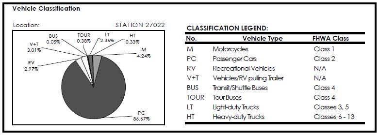
| Location: |
CLASSIFICATION LEGEND: |
|||
|---|---|---|---|---|
| STATION 27022 | No. | Vehicle Type | FHWA Class | |
| M | 4.24% | M | Motorcycles | Class 1 |
| PC | 86.67% | PC | Passenger Cars | Class 2 |
| RV | 2.9% | RV | Recreational Vehicles | N/A |
| V+T | 3.01% | V+T | Vehicles/RV pulling Trailer | N/A |
| BUS | 0.05% | BUS | Transit/Shuttle Buses | Class 4 |
| TOUR | 0.38% | TOUR | Tour Buses | Class 4 |
| LT | 2.36% | LT | Light-duty Trucks | Classes 3, 5 |
| HT | 0.33% | HT | Heavy-duty Trucks | Classes 6 - 13 |
To better reflect the types of vehicles and vehicle combinations that frequent recreational areas, the NPS developed a unique vehicle classification scheme to support their traffic database. The NPS vehicle classification scheme consists of eight vehicle types:
The NPS Traffic Database was designed to provide a means for linking with other NPS and FHWA databases, such as the Road Inventory Program (RIP) and Geographic Information System (GIS) databases. In Traffic Data Reports produced periodically for NPS units, the relationship between the NPS vehicle classification scheme and the FHWA vehicle classification scheme is indicated. An example is provided (figure 1) from the "Yellowstone National Park Traffic Package" within the NPS 2004 Traffic Data Report. It should be noted, however, that the current NPS traffic data program only calls for an 8-hour sample in one or two locations per monitored park. This may not be sufficiently representative in certain parks and conditions. 27
Table 2. Length-Based Vehicle Classification in British Columbia
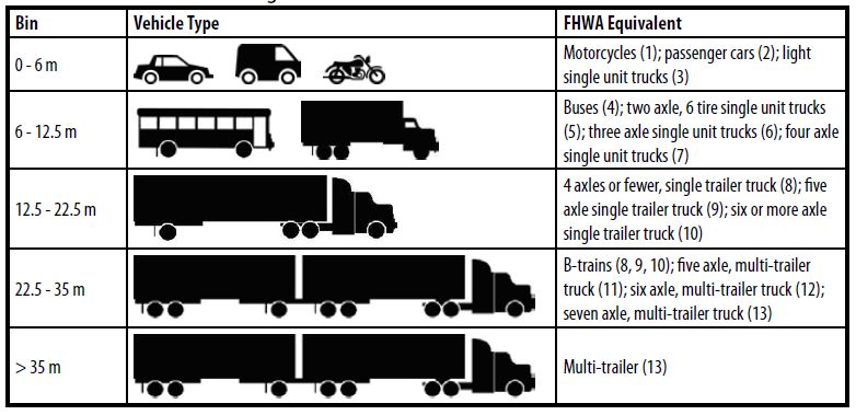
| Bin | Vehicle Type/FHWA Equivalent |
|---|---|
| 0 - 6 m | Motorcycles (1); passenger cars (2); light single unit trucks (3) |
| 6 - 12.5 m | Buses (4); two axle, 6 tire single unit trucks (5); three axle single unit trucks (6); four axle single unit trucks (7) |
| 12.5 - 22.5 m | 4 axles or fewer, single trailer truck (8); five axle single trailer truck (9); six or more axle single trailer truck (10) |
| 22.5 - 35 m | B-trains (8, 9, 10); five axle, multi-trailer truck (11); six axle, multi-trailer truck (12); seven axle, multi-trailer truck (13) |
| > 35 m | Multi-trailer (13) |
The FHWA vehicle classification scheme relies upon the identification of both the number of axles and the number of trailers in each vehicle. Automated methods for data capture (such as in-road sensors and supporting software) have been developed with these information needs in mind. A noted challenge for existing automated vehicle classification systems is the accurate classification of individual vehicles across the 13 categories when similarities exist in the number of axles. For example, a passenger car pulling a camper trailer may be misclassified as a four-axle single-unit or a single trailer truck.
Driven largely by the proliferation of electronic tolling systems in the United States (where vehicle type determines toll rates, which differ for commercial and non- commercial traffic), alternative technologies are in use and under development that can improve the accuracy of individual vehicle classification and support development of a wider range of vehicle classification schemes. Alternatives to axle-based data capture mechanisms are currently focused on vehicle length and vehicle profile. In-road or off-road non-intrusive sensors are used to detect vehicle length; vehicle lengths are then correlated with various vehicle classes such as car, single-unit truck, and combination truck.
The Minnesota DOT has initiated a pooled- fund study that will investigate issues related to length-based vehicle classification. The study objectives are to develop field test installation methods for loops to determine the most cost effective and best performing procedures and materials; determine the number of bins and the length spacing for each of those bins for uniform collection of length based classification data; and establish calibration standards for vehicle length based measurements. 28
The Province of British Columbia in Canada uses a length-based vehicle classification system. The relationship of British Columbia's vehicle classification scheme to FHWA's vehicle classification scheme is depicted in table 2. 29
Perhaps more appropriate for distinguishing the types of vehicles and vehicle combinations that frequent recreational areas are automated systems that capture the full vehicle profile. A variety of profiler systems are available commercially. The most advanced utilize Doppler radar, laser scanner, infrared light curtain and/or machine vision technologies to provide a two- or three- dimensional image of a vehicle that can then be appropriately categorized in a pre-defined classification scheme.
When conducting a review of literature related to traffic monitoring in recreational areas, researchers originally sought information on applied research and statistical methods that address traffic monitoring system coverage, data content, and data quality issues related to the composition and variability of recreational traffic. Not surprisingly, researchers observed a disproportionate focus on traffic monitoring in urban rather than recreational areas.
Much of the literature found to address recreational traffic monitoring considered: the use of recreational and/or seasonal factor groups, methods to support determination of recreational and/or seasonal factor groups, and the likely errors associated with factoring or annualizing short-term counts on roads with high-variability traffic.
The observed published literature served to define and characterize select recreational and/or seasonal factor groups currently in use at the State level. Most recently (2007), Byrne described the use of six seasonal factor groups in Vermont, three of which are devoted to recreational traffic:
In a report published in 2007, the New York State DOT described the use of three basic seasonal factor groups:
Within each of these main factor groups, two additional "minor" factor groups are provided to slightly increase or decrease the seasonal peaking characteristics. 31
In a related study published in 2000, Lingras et al. enumerates the seasonal factor groups that are used in the province of Alberta, Canada:
Table 3. Seasonal Factor Group Analysis in Delaware
| Factor Group | Monthly CV | Existing Permanent Count Stations | Permanent Count Stations Based on Variability | Recommended Permanent Count Stations |
|---|---|---|---|---|
| Urban | 7% | 24 | 4 | 27 |
| Rural | 16% | 16 | 13 | 19 |
| Recreational | 29% | 6 | 35 | 12 |
| Predominantly Recreational | 20% | 7 | 75 | 11 |
Shifting focus to the methods to support determination of recreational and/or seasonal factor groups, Faghri et al. reported recommendations for an integrated traffic monitoring system for Delaware in 1996. The authors recommended the use of four seasonal factor groups based on the monthly coefficient of variation (CV). Statistical analysis of the within-group variability was used to determine the required number of permanent count stations for an 80 percent confidence level and 10 percent error. The statistical analysis indicated that very few permanent count stations were required for urban and rural factor groups; the variability for the remaining two recreational factor groups indicated large required sample sizes, more than were possible given available resources. Taking these resource limitations into account, the authors provided final recommendations for the seasonal factor groups and number of permanent count stations (table 3). 33
One year later, Stamatiadis and Allen developed seasonal adjustment factors for vehicle classification counts for the State of Kentucky. Their research indicated that many States do not use seasonal adjustment factors for short-term vehicle classification counts. In this study, the authors used two years of vehicle classification data from Kentucky to develop class count factor groups. In their conclusions, the authors emphasized the importance of seasonal adjustment factors for accurate annual estimates. 34
In 2000, Aunet described the Wisconsin Department of Transportation's efforts to address traffic variability when developing seasonal factor groups. He emphasized that traffic data inherently has variability, both spatially and temporally, and recommended focusing traffic data analysis efforts on measuring or quantifying this variation and developing methods to account for it. He suggested a combination of approaches to develop seasonal factor groups and adjustment factors:
In 2003, Robichaud and Gordon reviewed traffic monitoring procedures for several Canadian provinces to provide recommendations to the British Columbia Ministry of Transportation. The authors reported on the results of studies in New Brunswick and Prince Edward Island that showed the use of regression was consistently more accurate for expanding short-term counts to annual estimates than the factoring method. However, the analysis of British Columbia data showed that factoring could be more accurate than regression if longer- duration short-term counts are used (on the order of 7 days once per year). 36
More recently (2004), Li et al. conducted a regression analysis to identify factors that most strongly affected seasonal traffic fluctuations in Florida. Currently the Florida DOT assigns short-term counts to a seasonal factor group based largely on spatial proximity to the permanent monitoring locations. The results of the analysis indicated that roadway functional class was not a significant factor, but the following were significant factors for seasonal traffic fluctuation:
These land use variables could be obtained from the planning departments and/or agencies.
A significant body of work related to the potential for errors when factoring short- term traffic counts, spanning nearly a decade, was authored by Satish C. Sharma. In 1993, Sharma and Allipuram used data from 61 permanent traffic monitoring locations in Alberta, Canada to analyze the frequency and duration of seasonal traffic counts. According to the authors, there is wide variation in how long and often seasonal counts are taken in the Canadian provinces. The researchers developed an algorithm that could be used to optimize the seasonal traffic count schedule based on three road types (i.e., commuter, average rural, recreational). 38
In 1996, Sharma et al. analyzed the tradeoffs in precision of annual traffic counts when using seasonal traffic counts. In this study, researchers examined the collection of counts for two, three, and four non-contiguous months. Seasonal traffic counts, or several short-term counts spread throughout the year, are sometimes used as an alternative to a single short-term count when there are significant or unknown seasonal fluctuations. The study found the following errors at a 95% confidence level:
During the same year, Sharma et al. analyzed data from several permanent count stations in Minnesota to determine the effects of various factors on the statistical precision of AADT estimates. Consistent with other studies, researchers found that the AADT estimation errors are very sensitive to the assignment effectiveness (i.e., the correctness with which a sample site has been assigned to a factor group). Additionally, the authors indicated that traffic monitoring agencies should place more emphasis on accurately assigning short-term counts to factor groups, rather than on conducting longer duration counts (e.g., 72-hour counts). The study findings from Minnesota were confirmed with permanent count data from Alberta and Saskatchewan analyzed in the same year. 40
In two related reports published in 2000 and 2001, Sharma et al. reported results of various analysis techniques to estimate annual average traffic counts on low-volume roads. Researchers found that artificial neural networks were more favorable for AADT estimation than the traditional factor approach. In particular, one advantage of the neural network approach is that the definition and designation of seasonal factor groups is not necessary. Results also indicated a clear preference for two 48-hour short-term counts as compared to other frequencies (one or three) or durations (24- or 72-hour). 41 42
In 1997, Davis reviewed the procedures used to estimate the accuracy of "annualized" short-term counts and found that many attempts failed to include the error from using incorrect seasonal or day-of-week adjustment factors. Based on his research, Davis recommended the use of seasonal counts (i.e., short-term counts taken during several seasons of the year) to provide solid prior information for assigning short-term counts to a seasonal factor group. 43
Most recently (2007), Lewis and Albright described the errors associated with the application of default traffic count adjustment factors. In this case, city engineers were using default national factors in the Highway Capacity Manual to adjust average weekday traffic counts (AWDT) to AADT counts. The authors indicated that the default national factors were different than those provided by the State's traffic monitoring agency. Further, the authors suggested improvements to the States' seasonal factor groups which are currently based on area type and roadway functional class. 44
Two additional publications are worthy of note. In 1980, Erickson et al. considered automatic time-interval counts for use in the planning and management of recreational areas. The authors collected hourly directional counts in the Daniel Boone National Forest using punch cards over a 4-month period. An interesting finding from this effort was that, at several locations, the entering traffic had much different traffic peaking patterns than exiting traffic. The authors also highlighted the variability throughout the data collection period that was presumably due to adverse weather conditions. 45
In 2005, Dunning documented the impacts of transit service on traffic conditions in national parks and gateway communities. Dunning described the difficulties of monitoring changes in visitation due to management actions, such as the introduction of transit services. She indicated that changing methods for monitoring visitation traffic can confound an accurate before-after comparison. Additionally, she noted that in parks where traffic counts and a vehicle occupancy multiplier are used to estimate visitation, the assumed vehicle occupancy may also change in the "after" evaluation period. She concluded that visitation counts could give general insights but could not fully describe the impacts of transit service. 46
10. http://www.blm.gov/wo/st/en/info/About_BLM.html, accessed July 15, 2009.
11. Placchi, Jack. Bureau of Land Management Perspective. Recreational Traffic Monitoring Workshop. June 2009.
12. Fish and Wildlife Service Agency Overview: Conserving the Nature of America. November 2008.
13. https://www.fs.fed.us, accessed July 15, 2009.
14. https://www.nps.gov/aboutus, accessed July 15. 2009.
15. Kathryn Gunderson. National Park Service Practices and Perspectives. Recreational Traffic Monitoring Workshop. June 2009.
16. Butch Street. National Park Service Practices and Perspectives. Recreational Traffic Monitoring Workshop. June 2009.
17. Traffic Monitoring Guide. FHWA-PL-01-021. Office of Highway Policy Information, Federal Highway Administration, U.S. Department of Transportation. Washington D.C. May 2001.
18. Guidelines for Traffic Data Programs. American Association of State highway and Transportation Officials. Washington D.C. 1992.
19. Highway Performance Monitoring System Field Manual for the Continuing Analytical and Statistical Database. Office of Highway Policy Information, Federal Highway Administration, U.S. Department of Transportation. Washington D.C. May 2005.
20. https://www.fhwa.dot.gov/policyinformation/, accessed December 17, 2008.
21. Kashuba, Ed. Vehicle Classification System: FHWA Perspective. North American Travel Monitoring Exposition and Conference (NATMEC). August 2000.
22. https://www.fhwa.dot.gov/policyinformation/, accessed December 17, 2008.
23. AASHTO Green Book - A Policy on Geometric Design of Highways and Streets, 5th Edition. American Association of State and Highway Transportation Officials. November 2004.
24. Highway Capacity Manual. Transportation Research Board, National Research Council. Washington D.C. 2000.
25. https://www-fars.nhtsa.dot.gov/Vehicles/VehiclesAllVehicles.aspx, accessed December 17, 2008.
26. Clayton, Alan, Jeannette Montufar, Dan Middleton, and Bill McCauley. Feasibility of a New Vehicle Classification System for Canada. North American Travel Monitoring Exhibition and Conference (NATMEC). August 2000.
27. National Park Service. 2004 Traffic Data Report. 2005.
28. http://www.pooledfund.org/projectdetails.asp?id=416&status=4, accessed December 18, 2008.
29. http://www.th.gov.bc.ca/trafficData/vcc, accessed December 18, 2008.
30. Bernard F. Byrne. Revised Method for Estimating Design Hourly Volumes in Vermont. Transportation Research Record 1993, Transportation Research Board of the National Academies, Washington, D.C., 2007, pp. 23-29.
31. 2007 Traffic Data Report for New York State, New York State Department of Transportation, available at https://www.nysdot.gov/divisions/ engineering/technical-services/highway-data-services/traffic-data.
32. Pawan Lingras, Satish C. Sharma, Phil Osborne, and Iftekhar Kalyar. Traffic Volume Time-Series Analysis According to the Type of Road Use. Computer-Aided Civil and Infrastructure Engineering, Volume 15, 2000, pp. 365-373.
33. Ardeshir Faghri, Martin Glaubitz, and Janaki Parameswaran. Development of Integrated Traffic Monitoring System for Delaware. Transportation Research Record 1536, Transportation Research Board, National Academies, Washington, D.C., 1996, pp. 40-44.
34. Nikiforos Stamatiadis and David L. Allen. Seasonal Factors Using Vehicle Classification Data. Transportation Research Record 1593, Transportation Research Board, National Academies, Washington, D.C., 1997, pp. 23-28.
35. Bruce Aunet. Wisconsin's Approach to Variation in Traffic Data. Paper presented at NATMEC 2000 Conference, 14 pages.
36. Karen Robichaud and Martin Gordon. Assessment of Data-Collection Techniques for Highway Agencies. Transportation Research Record 1855, Transportation Research Board of the National Academies, Washington, D.C., 2003, pp. 129-135.
37. Min-Tang Li, Fang Zhao, and Yifei Wu. Application of Regression Analysis for Identifying Factors That Affect Seasonal Traffic Fluctuations in Southeast Florida. Transportation Research Record 1870, Transportation Research Board of the National Academies, Washington, D.C., 2004, pp. 153-161.
38. Satish C. Sharma and Reddy. R. Allipuram. Duration and Frequency of Seasonal Traffic Counts. Journal of Transportation Engineering. Volume 119, No. 3, May/June 1993, pp. 344-359.
39. Satish C. Sharma, Peter Kilburn, and Yongquiang Wu. The precision of average annual daily traffic volume estimates from seasonal counts: Alberta example. Canadian Journal of Civil Engineering, Volume 23, 1996, pp. 302- 304.
40. Satish C. Sharma, Brij M. Gulati, and Samantha N. Rizak. Statewide Traffic Volume Studies and Precision of AADT Estimates. Journal of Transportation Engineering, Volume 122, No.6, November/December 1996, pp. 430-439.
41. Satish Sharma, Pawan Lingras, Fei Xu, and Peter Kilburn. Application of Neural Networks to Estimate AADT on Low-Volume Roads. Journal of Transportation Engineering, Volume 127, No. 5, September/October 2001, pp. 426-432.
42. Satish C. Sharma, Pawan Lingras, Guo X. Liu, and Fei Xu. Estimation of Annual Average Daily Traffic on Low-Volume Roads: Factor Approach Versus Neural Networks. Transportation Research Record 1719, Transportation Research Board of the National Academies, Washington, D.C., 2000, pp. 103-111.
43. Gary A. Davis. Accuracy of Estimates of Mean Daily Traffic: A Review. Transportation Research Record 1593, Transportation Research Board of the National Academies, Washington, D.C., 1997, pp. 12-16.
44. Martin Lewis and David Albright. Evaluating the Highway Capacity Manual's Adjustment Factor for Annual Weekday to Annual Average Daily Traffic: Applying a Consistent Traffic Data Methodology. Transportation Research Record 1993, Transportation Research Board of the National Academies, Washington, D.C., 2007, pp. 117-123.
45. D.L. Erickson, C.J. Liu, and H.K. Cordell. Automatic, Time-Interval Traffic Counts for Recreation Area Management Planning. Paper presented at the National Outdoor Recreation Trends Symposium, Durham, NH, April 20-23, 1980, 10 pages.
46. Anne E. Dunning. Impacts of Transit in National Parks and Gateway Communities. Transportation Research Record 1931, Transportation Research Board of the National Academies, Washington, D.C., 2005, pp. 129-136.
Stay up to date
Sign up for announcements on grant opportunities, training, and webinars.