


| AP | Availability Payment |
| BCA | Benefit Cost Analysis |
| BS | Balance Sheet |
| CF | Cash Flow |
| CFADS | Cash Flows Available to Debt Service |
| DSCR | Debt Service Coverage Ratio |
| DSRA | Debt Service Reserve Account |
| GPL | General Purpose Lanes |
| IRI | International Roughness Index |
| IRR | Internal Rate of Return |
| ML/TL | Managed Lanes or Tolled Lanes |
| MMRA | Major Maintenance Reserve Account |
| O&M | Operations and Maintenance |
| PDBCA | Project Delivery Benefit-Cost Analysis |
| P&L | Profit & Loss |
| PSC | Public Sector Comparator or Conventional Delivery |
| P3 | Public-Private Partnership |
| V/C | Volume/Capacity Ratio |
| VDF | Volume Delay Function |
| WACC | Weighted Average Cost of Capital |
This section describes the use of the detailed input sheets. Please refer to Section 0 for a discussion of the simplified inputs sheet.
The detailed input sheets can be accessed through the Model Navigator. The following panel with the various input sheets will appear upon clicking on the Inputs button in the Model Navigator.
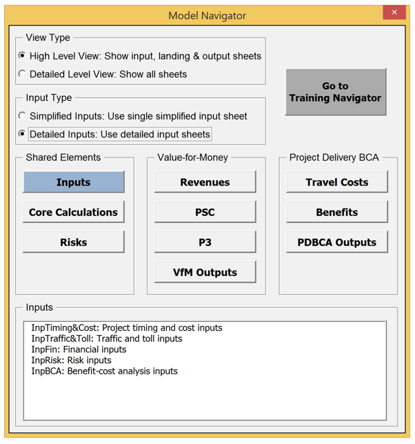
Model Navigator
This model navigator screenshot displays the detailed inputs at a high level view, including input timing and cost, input traffic and tolls, input finances, input risk and input BCA.
Alternatively, users can use the usual Excel navigation features to access the different sheets. Users will be required to input data in the different input sheets for the PSC and the P3 delivery models. For the Delayed PSC delivery model, the user only needs to input start and duration of pre-construction (see below), with all other values being equal to the PSC.
Users are only expected to provide inputs in cells that are yellow-shaded (for project specific inputs) or orange-shaded (for non-project specific inputs)
This sheet seeks user inputs for the timeline and basic cost for the various delivery models to be considered in the analysis.
In this section, the user will input the specific years in which project phases begin, as well as the duration of each phase for the various delivery models. Users should input data in the yellow-shaded cells.
The following provides sample timing inputs:
| Construction and operations timing | Unit | PSC | Delayed PSC | P3 |
|---|---|---|---|---|
| Pre-construction start year | year # | 2018 | 2023 | 2018 |
| Pre-construction duration | years | 2 | 2 | 2 |
| Construction start year | year # | 2020 | 2025 | 2020 |
| Construction duration | years | 4 | 4 | 3 |
| Operations start year | year # | 2024 | 2029 | 2023 |
| Operations duration | years | 40 | 35 | 41 |
| Operations end year | year # | 2063 | 2063 | 2063 |
In this section of the InpTiming&Cost sheet, users will input all major costs items for each of a project's phases:
The user should enter all costs in dollar terms in the indexation base year (see section 4.1.3 below). Users should only input data in the yellow-shaded cells. The model contains the following cost items:
For each of the above cost items, the following inputs are required:
P3 transferred cost: Please enter the share of the P3 cost amount that will be transferred from the Agency to the P3 concessionaire (in percent). Furthermore, users are expected to provide No Build annual O&M costs (in thousands of dollars per year), which are used to calculate the No Build O&M cost savings achieved by doing the project. The No Build annual O&M amount should include all operational costs that will not have to be incurred if the project is undertaken, including annualized costs of any contributions towards major maintenance.
Please note that P3-VALUE 2.2 does not adjust O&M costs for traffic. In other words, even if traffic is lower than expected, the O&M costs remain the same.
This section of the worksheet prompts user input for escalation and indexing for costs and revenues. The user must input the indexation base year and should adjust the indexation rate as appropriate for each of the project costs and revenue sources. Please note that all input cost and revenue sources are assumed to be in nominal terms, using the indexation base year input as its base year. The indexation base year is also used as the base year for NPV calculations (see section 4.3.2). The following is an example of input for this section:
| Escalation | Constant | Unit |
|---|---|---|
| Indexation base year | 2018 | year # |
| Indexation rate - Construction | 2.00% | % p.a. |
| Indexation rate - Operations | 2.00% | % p.a. |
| Indexation rate - Toll rates | 2.00% | % p.a. |
| Indexation rate - CPI | 2.00% | % p.a. |
| Indexation rate - Subsidy | 2.00% | % p.a. |
| Allowable share of indexed O&M component in availability payment | 2.00% | % |
| Indexation rate - O&M component of availability payment | 2.00% | % p.a. |
This section of the worksheet presents non-changeable technical inputs. The user is not expected to change any of these inputs and can ignore them while performing a VfM analysis and PDBCA. Non-changeable inputs include view mode, input mode, and navigator labels (used in a macro to switch from detailed-level to high-level view, from detailed inputs to simplified inputs, and from Model Navigator to Training Navigator), timeline labels (used to provide visual timelines in each calculation sheet) and a number of constants.
| Labels | Constant | Unit |
|---|---|---|
| Navigator labels | ||
| View mode ("Detailed Level View" or "High Level View") - Macro driven | Detailed Level View | switch |
| Input mode (0 = Detailed inputs, 1 = Simplified inputs) - Macro driven | 0 | switch |
| Input mode details | Detailed Inputs | switch |
| Navigator option ("Model Navigator" or "Training Navigator") - Macro driven | Model Navigator | switch |
| View of model | Detailed Level View | switch |
| Timeline labels | ||
| Timeline Labels for PSC and P3 | ||
| Project initiation period | label | |
| Pre-construction period | Pre-Constr. | label |
| Construction period | Construction | label |
| Operations period | Operations | label |
| Post-operations period | Post-Ops. | label |
| Timeline Labels for Delayed PSC | ||
| Project initiation period | Delayed | label |
| Pre-construction period | Pre-Constr. | label |
| Construction period | Construction | label |
| Operations period | Operations | label |
| Post-operations period | Post-Ops. | label |
The constants include consumer surplus factor (equal to ½, please refer to Part II 5.11 explaining the calculation of consumer surplus), the number of directions in bidirectional traffic (equal to 2 directions), the variance quadratic factor, uniform variance factor, triangular variance factor (factors used in the calculation of variance for pure risks), goal seek precision multiplier (input used for the Model Optimizer), and various units.
| Constants | Constant | Unit |
|---|---|---|
| Consumer surplus factor (for PDBCA) | 0.5000 | factor |
| Number of directions in bidirectional traffic | 2 | directions |
| Variance quadratic factor | 2.0000 | factor |
| Uniform variance factor | 12.0000 | factor |
| Triangular variance factor | 18.0000 | factor |
| Goal seek precision multiplier | 1 | # |
| Units in a hundred | 100 | units |
| Units in a thousand | 1,000 | units |
| No. of days in a year | 365 | days |
| Months in a year | 12 | months |
| Units in a million | 1,000,000 | units |
Furthermore, the Model Optimizer requires a number of numerical inputs, which are listed below.
| Model tolerance & optimization parameters | Constant | Unit |
|---|---|---|
| Model check tolerance level | 0.0010 | tolerance |
| Model check tolerance level amplifier | 0.1000 | tolerance |
| P3 - WACC for initial AP estimation in macro | 8.00% | % p.a. |
| P3 - WACC for initial subsidy / concession fee estimation in macro | 10.00% | % p.a. |
Please note that the non-changeable technical inputs are not accessible under the high-level view.
This sheet seeks user inputs for traffic volumes, toll rates, traffic characteristics and shares, speed, and roadway capacity.
The model enables users to input bidirectional P50 (or most likely) weekday traffic data for up to five different input years over the project analysis period. Users must provide traffic data for the No Build and Build (Managed Lanes or Tolled Lanes and General Purpose Lanes separately) for the model start year (PSC or P3 pre-construction start year, whichever is earlier). Users may also provide up to four additional traffic data points by entering the relevant traffic data point year and forecast. If the project is a simple toll road (as opposed to a Managed Lanes facility), traffic inputs on the General Purpose Lanes (GPL) should be zero. If the project is not tolled, traffic inputs on the Managed Lanes or Tolled Lanes (ML/TL) should be zero. If the project is a managed lane project, the user will input both tolled traffic (on ML/TL) and non-tolled traffic (GPL). Please note that Build traffic (Managed Lanes or Tolled Lanes and General Purpose Lanes traffic combined) should be equal to or exceed No Build traffic. The following shows sample inputs for a project involving the expansion of an existing facility to accommodate managed lanes along with free GPLs.
Users are also expected to provide the annual traffic growth after the last input year. This input is used to project traffic beyond the last year of input. The following shows sample inputs. In the sample inputs, "> 2050" refers to traffic growth after 2050, the last year of input in the considered example.
The units are thousands of vehicles per weekday.
| Bidirectional traffic forecast | Unit | Year | No Build | ML/TL | GPL |
|---|---|---|---|---|---|
| Bidirectional P50 weekday daily traffic in model start year (2017) | 000s | 2017 | 120.0 | 25.0 | 105.0 |
| Bidirectional P50 weekday daily traffic in input year 2 | 000s | 2020 | 127.0 | 30.0 | 110.0 |
| Bidirectional P50 weekday daily traffic in input year 3 | 000s | 2030 | 138.0 | 35.0 | 121.0 |
| Bidirectional P50 weekday daily traffic in input year 4 | 000s | 2040 | 150.0 | 40.0 | 131.0 |
| Bidirectional P50 weekday daily traffic in input year 5 | 000s | 2050 | 158.0 | 45.0 | 142.0 |
| Annual traffic growth after last input year | % p.a. | > 2050 | 0.50% | 1.00% | 0.50% |
The model has a built-in feature to ensure that project daily traffic does not exceed the facility's daily capacity. Please refer to Part II 5.3 for more detail on this feature.
The model allows to model a (linear) traffic ramp-up through two ramp-up parameters: Ramp-up starting traffic and ramp-up period duration. As an example, if traffic is expected to reach 50%, 80%, 90%, and 100% of post-ramp up traffic in year 1, 2, 3, and 4, respectively, the ramp-up starting traffic is 50%, whereas the ramp-up period duration would be four years
| Ramp-up | Unit | PSC | Delayed PSC | P3 |
|---|---|---|---|---|
| Ramp-up starting traffic (% of post-ramp up traffic) | % | 50.00% | 50.00% | 50.00% |
| Ramp-up period duration | years | 5 | 5 | 5 |
Users will need to input the toll rates for 2- (passenger cars), and 4-axle (trucks/buses) vehicles for weekday peak, weekday off-peak and weekends, for the No-Build, ML/TL, and GPL. The following shows sample inputs.
| Toll rates and leakage | Unit | No Build | ML/TL | GPL |
|---|---|---|---|---|
| 2 axle vehicles toll rates - Weekday - Peak | USD / vehicle | 0.00 | 4.00 | 0.00 |
| 2 axle vehicles toll rates - Weekday - Off-peak | USD / vehicle | 0.00 | 2.00 | 0.00 |
| 2 axle vehicles toll rates - Weekend | USD / vehicle | 0.00 | 2.00 | 0.00 |
| 4+ axle vehicles toll rates - Weekday - Peak | USD / vehicle | 0.00 | 6.00 | 0.00 |
| 4+ axle vehicles toll rates - Weekday - Off-peak | USD / vehicle | 0.00 | 4.00 | 0.00 |
| 4+ axle vehicles toll rates - Weekend | USD / vehicle | 0.00 | 4.00 | 0.00 |
Note that HOV toll exemptions are not accounted for, either for buses or for carpools.
In addition, the user is requested to enter the expected toll revenue leakage (as a percentage of total toll revenues).
| Toll revenue leakage | 1.00% | % |
Besides the traffic and toll inputs, the PDBCA module also requires other traffic-related inputs. First, users are expected to provide a traffic sensitivity factor, which determines what share of the growth in traffic (i.e., P50 (or most likely) traffic above No Build base year traffic) will be considered in the PDBCA module. This traffic sensitivity factor captures uncertainty in traffic projections. The factor is applied to all traffic above the No Build base year traffic, both for the Build and No Build scenarios. If the sensitivity factor is set to 0%, the base year No Build traffic will be applied in all years (no traffic growth) to both the No Build and Build scenarios. The model allocates the No Build base year traffic on a pro rata basis to the Managed Lanes or Tolled Lanes and General Purpose Lanes using the weekday daily traffic inputs. If the traffic sensitivity factor is set to 100%, the model directly uses the weekday daily traffic inputs. If a value between 0% and 100% (or above 100% for an upside sensitivity analysis) is selected, the factor is applied to all No Build and Build traffic above the No Build base year traffic.
In the VfM analysis, the uncertainty is captured through the revenue uncertainty adjustment (for the PSC) and the cost of capital (for P3). Please refer to Part II for a more detailed discussion on risks and uncertainty.
| Traffic sensitivity factor for PDBCA (applies to traffic above No Build base year traffic) | 100.00% | % |
Furthermore, users will be expected to provide information on the facility's segment length. The number of representative weekdays has a default value of 250 days per year (non-project specific default inputs are orange-shaded). The number of weekend days or holidays in a year is calculated automatically.
| Segment length | 20 | miles |
| Weekdays in a year | 250 | days |
| Weekend days / holidays in a year | 115 | days |
Users will also need to input the number of unidirectional peak hours in a day, and the number of uni-directional off-peak hours in a day. For example, a radial highway may experience an AM peak period of 3 hours in the direction of the central business district while a circumferential highway may experience an AM peak period of 3 hours and a PM peak period of 3 hours, i.e. a total of 6 hours of peak traffic. The following shows sample inputs.
| No. of unidirectional peak hours in a day (during AM, PM or combined) | 3 | hours |
| No. of unidirectional off-peak hours in a day | 15 | hours |
In the above example, the amount of traffic carried by the roadway for 6 hours at night (e.g., between 12:00 AM and 6:00 AM) is insignificant. Therefore, the off-peak period is 15 hours. The model requires users to input only the number of hours with significant traffic in order to ensure that off-peak congested speed is representative of real world conditions.
Next, users will need to input the number of lanes per direction as well as the relative share of unidirectional peak traffic (as a percentage of weekday traffic) and weekend traffic (as a percentage of weekday traffic), for the No Build, Managed Lanes/Tolled Lanes, and General Purpose Lanes. As the combined weekday traffic needs to be 100%, the unidirectional off-peak traffic percentage is calculated directly from the unidirectional peak traffic percentage. Sample inputs are shown below.
| Traffic and project characteristics | Unit | No Build | ML/TL | GPL |
|---|---|---|---|---|
| No. of lanes per direction | lanes | 3 | 2 | 3 |
| No. of lanes in both directions | lanes | 6 | 4 | 6 |
| Unidirectional peak traffic percentage | % | 30.00% | 30.00% | 30.00% |
| Unidirectional off-peak traffic percentage | % | 70.00% | 70.00% | 70.00% |
| Weekend traffic (% of weekday traffic) | % | 60.00% | 60.00% | 60.00% |
In addition, users must enter 2-axle vehicle percentages for peak, off-peak, and the weekend. The 4+ axle traffic shares are calculated automatically using the 2 axle traffic shares. The following shows sample inputs.
| Traffic shares | Unit | No Build | ML/TL | GPL |
|---|---|---|---|---|
| 2 axle vehicle percentage - Peak | % | 95.00% | 100.00% | 95.00% |
| 4+ axle vehicle percentage - Peak | % | 5.00% | 0.00% | 5.00% |
| 2 axle vehicle percentage - Off-peak | % | 90.00% | 100.00% | 90.00% |
| 4+ axle vehicle percentage - Off-peak | % | 10.00% | 0.00% | 10.00% |
| 2 axle vehicle percentage - Weekend | % | 95.00% | 100.00% | 95.00% |
| 4+ axle vehicle percentage - Weekend | % | 5.00% | 0.00% | 5.00% |
In order to calculate travel time savings, the model requires users to provide free flow speeds for both 2 axle and 4+ axle vehicles. The following shows sample inputs.
| Highway free flow speeds | Unit | No Build | ML/TL | GPL |
|---|---|---|---|---|
| Highway free flow speed - 2 axle | miles / hour | 65 | 70 | 70 |
| Highway free flow speed - 4+ axle | miles / hour | 60 | 65 | 65 |
Beyond traffic and speed inputs, the model requires additional information regarding the relation between speeds and traffic volumes to accurately predict delays due to high traffic volumes. More specifically, the model uses a volume delay function (VDF). Its default parameters are provided below, as well as the Level of Service C (LOS C) lane vehicle capacity (expressed as thousands of passenger car equivalents per lane per hour).
| Volume delay function | Constant | Unit |
|---|---|---|
| Bureau of Public Road Volume Delay Function parameter Alpha | 0.15 | factor |
| Bureau of Public Road Volume Delay Function parameter Beta | 4.00 | factor |
| Lane vehicle capacity at LOS C | 1.50 | 000s/lane/hour |
The capacity and VDF parameters used by the regional travel demand model (maintained by the Metropolitan Planning Organization) may be used as inputs for P3-VALUE 2.2 in order to ensure that the estimated traffic speeds and capacities are consistent. The user may alternatively use the Highway Capacity Manual to estimate capacity based on roadway characteristics if lane vehicle capacity information cannot be obtained from the travel demand model documentation. FHWA recommends using LOS C capacity to estimate congested speeds 5.
As mentioned earlier, the model contains a built-in feature that ensures that future daily traffic does not exceed the facility's daily capacity. To determine the facility's daily capacity, the model requires two additional inputs: 1) An hourly-to-daily capacity conversion factor and 2) the ratio of LOS E capacity to LOS C capacity. Default inputs are provided for the No Build, Managed Lanes/Tolled Lanes, and General Purpose Lanes separately.
| Capacity | Unit | No Build | ML/TL | GPL |
|---|---|---|---|---|
| Hourly-to-daily capacity conversion factor | factor | 15 | 10 | 15 |
| Ratio of LOS E capacity to LOS C capacity* | factor | 1.33 | 1.00 | 1.33 |
| * LOS E = maximum vehicle throughput, LOS C = vehicle throughput at or near free flow | ||||
In the traffic and toll input sheet, there is a daily traffic capacity breach check that indicates whether the daily traffic assumptions lead to traffic beyond capacity. If the check is green, projected traffic is less than the facility's capacity. If the check is orange, projected traffic exceeds the facility's capacity, in which case the model automatically constrains traffic at capacity. This check is also included in the "error checks and alerts" summary at the top of each input and calculation sheet.
Please note that the volume and capacity inputs are not accessible under the high-level view.
It is to be noted that P3-VALUE 2.2 has certain limitations with regard to the type of projects it can analyze. For example, there is only one lane type and associated traffic input for the No Build. If the No Build contains both high occupancy vehicle (HOV) lanes and general purpose lanes (GPL), the user would need to combine both types of traffic into a single input. While the combined traffic volumes can be directly input, the vehicle occupancy for the No Build would need to be adjusted to represent both sets of lanes. In addition, HOV lanes and the GPLs may in reality have different congested speeds. Since a single Volume Delay Function (VDF) would be applied to the combined traffic, the estimated congested speeds will not reflect actual conditions. The VDF will overestimate the speed of GPL traffic and underestimate the speed of HOV traffic. Therefore, use of P3-VALUE 2.2 for this type of project will not provide an accurate representation of congestion delays in the No Build scenario.
A second limitation of P3-VALUE 2.2 is that it assumes that Build traffic (all lanes combined) is higher than, or at least equal to, No Build traffic. However, the presence of a high toll could reduce traffic in the Build alternatives relative to the No Build case. In the presence of a relatively high toll, traffic may divert to other facilities. P3-VALUE 2.2 cannot be used in such a case, since a basic assumption in the model is that Build traffic will be equal to or higher than No Build traffic. A possible way to overcome this limitation might be to run the travel demand model using the higher toll to determine the No Build traffic under these conditions. Such an approach would allow for a comparison between the Build and No Build alternatives and ensures that the Build traffic is at least as much as the No Build traffic.
P3-VALUE 2.2 also cannot directly analyze reversible lanes. If the user wishes to analyze reversible lanes, it may be possible to conduct two separate analyses, one for each direction of travel, and combine the results.
Projects that are conducted to upgrade structurally deficient infrastructure (such as bridge replacement) or provide an emergency evacuation route may not yield a significant increase in travel cost savings compared to the No Build. If the user wishes to analyze such projects using P3-VALUE 2.2, the user may, for example, calculate the additional safety benefits exogenously and add them to the benefits calculated by P3-VALUE 2.2 in order to perform a more complete evaluation of costs and benefits.
The InpFin is the input sheet where users enter funding and financing inputs. This input sheet has many critical inputs, which can dramatically affect the outputs.
P3-VALUE 2.2 enables users to perform three different comparisons between PSC (Conventional Delivery) and P3, which are listed below. The first two comparison scenarios both consider a tolled highway, whereas the third scenario considers a non-tolled highway.
For the PSC in the first comparison scenario, the Agency will make use of conventional delivery such as a design-bid-build (DBB) or design-build (DB) contract, with all toll revenues directly flowing to the Agency. If the project is procured as a P3, the P3 concessionaire will be responsible for the construction and operation of the facility but will also retain all toll revenues ("toll concession"). Furthermore, the P3 concessionaire may require a subsidy or may be willing to pay a concession fee, depending on the project.
For the second scenario, the PSC has exactly the same structure as the PSC under the first scenario. Under P3 for this second scenario, the P3 concessionaire will still be responsible for the construction and operation of the facility, but will not retain the toll revenues, which will flow to the Agency. In return, the Agency will pay the P3 concessionaire an availability payment for the duration of the concession period.
The last scenario is exactly the same as the second scenario, except that there is no tolling. This means that the Agency will not be able to use toll revenues to pay for the facility. Compared to the second scenario, the P3 concessionaire will not observe any real difference, as it will still receive a fixed availability payment from the Agency.
Users can select one of the above comparison scenarios using the dropdown menu at the top left of the InpFin input sheet (cell F6). The selected scenario is indicated with a ▼ symbol, as shown below.
| Active scenario --> | ▼ | |||
|---|---|---|---|---|
| Active scenario selection --> | PSC: Tolled, P3: Toll concession |
PSC: Tolled, P3: Toll concession |
PSC: Tolled, P3: Availability Payment |
PSC: Not tolled, P3: Availability Payment |
In this section, the user will provide information regarding discounting, taxation, and competitive neutrality adjustment.
Two elements are important for discounting. First, a net present value (NPV) always refers to a point in time. Therefore, the model needs to know what reference year will be used for NPV calculations. The second element required to discount cash flows is the discount rate. In the VfM analysis and the risk analysis, the model uses a project risk-free discount rate to calculate the NPV of costs and revenues to the Agency. Cash flows to the P3 concessionaire, however, are discounted at the Weighted Average Cost of Capital (WACC). The project risk-free discount rate reflects the time value of money and related uncertainties and risks (i.e., not including project risks), just like any interest rate. The term "project risk free" indicates that the discount rate does not reflect uncertainties and risks that are specific to a project. On the other hand, an interest rate in a project finance structure would reflect such project specific risks. The Agency's borrowing rate can potentially be used as a proxy for the project risk-free discount rate.
For the NPV calculations in the PDBCA, the model uses the social real discount rate. However, determining the social real discount rate can be challenging. Theoretically, the social discount rate should represent the benefits foregone from alternative use of those funds by the Agency or government. In practice, it may be difficult to determine the right value. As guidance, the user should use the state or Agency's social discount rate or follow the Federal Office of Management and Budget's (OMB) Circular A-94.
| Discounting | Constant | Unit |
|---|---|---|
| NPV base year (same as "Indexation base year" in InpTiming&Cost) | 2018 | year # |
| Project risk-free discount rate (for VfM analysis) | 4.00% | % p.a. |
| Social real discount rate (for PDBCA) | 2.00% | % p.a. |
Regarding tax, the model provides the option to input both federal and state tax rates for the P3 concessionaire. Whether or not the P3 concessionaire will pay tax depends on its legal structure. The model allows for a tax pass-through to the parent company, meaning that the parent company could take advantage of tax losses generated by the project. If no tax pass-through is considered, the model allows the concessionaire to carry forward losses to future tax periods for a specified number of years. The following shows sample tax inputs.
| Tax | Constant | Unit |
|---|---|---|
| Tax pass-through to parent company? | FALSE | switch |
| Tax losses expiration period (only relevant if no
tax pass-through to parent company) |
20 | years |
| P3 - State tax rate | 10.00% | % |
| P3 - Federal tax rate | 25.00% | % |
Furthermore, to ensure a fair comparison between PSC and P3, the model enables users to apply a competitive neutrality adjustment for the following elements:
The competitive neutrality adjustment is included to ensure an apples-to-apples comparison between the PSC and P3. For example, if the P3 is more expensive due to taxation that will flow back to the government, the increased cost due to taxation should logically not negatively impact the evaluation. To offset this effect, the same tax liability can either be added to the PSC as a cost or alternatively subtracted from the P3 cost. Depending on their perspective and preference, users can decide to ignore the competitive neutrality adjustment, or to include a partial adjustment for, for example, only state tax. The following shows sample competitive neutrality adjustment inputs.
If the Agency self-insures under PSC while requiring insurance from the P3 concessionaire in case of a P3 can lead to a similar issue. P3-VALUE 2.2 allows the user to estimate the value of self-insurance (as a percentage of the construction/O&M costs) in order to adjust the VfM results accordingly. Furthermore, the model allows users to incorporate different credit subsidies under the PSC and P3 into the competitive neutrality adjustment.
| Competitive neutrality adjustment | Constant | Unit |
|---|---|---|
| State tax considered for competitive neutrality adjustment? | TRUE | switch |
| Federal tax considered for competitive neutrality adjustment? | TRUE | switch |
| Construction self-insurance (% of transferred construction costs) | 0.00% | % |
| O&M and major maintenance self-insurance (% of transferred O&M costs) | 0.00% | % |
| PSC credit subsidy at financial close | - | USD k |
| P3 credit subsidy at financial close | - | USD k |
Users only need to provide inputs for the yellow-shaded cells in columns I, J, or K. Cells and/or columns that are greyed-out relate to comparison scenario other than the one selected in cell F6 (see above). The list below provides an explanation of the various inputs required.
Please note that the above listed inputs determine the financing conditions of the PSC and P3. When inputting these values, users should be aware that the financing conditions should reflect the financiers' exposure to risks (including revenue risk for P3 toll concessions). As explained in the section 4.4 on Risk Inputs, P3-VALUE 2.2 contains the option to use market-based financing conditions to quantify the revenue uncertainty adjustment and lifecycle performance risk premium.
The inputs listed below are used to define the three comparison scenarios. Users are not expected to change these inputs, which is why these cells have been grayed out.
Please note that the comparison scenario definition inputs are not accessible under the high-level view.
In the InpRisk sheet, users are expected to provide project risk information. P3-VALUE 2.2 recognizes three separate risk categories: pure risk, base variability risk, and lifecycle performance risk. Furthermore, the model uses a revenue uncertainty adjustment to account for revenue uncertainty. For a detailed discussion on how these risks are valued in the tool, please refer to Part II Section. The inputs required for each risk category are discussed below.
Pure risks are also known as event risks and refer to individual risk events, such as an accident at the construction site. As a first input, the user must determine what probability level should be used for the pure risk analysis. The probability level is input as a percentage. Based on this percentage, the model determines the value of the pure risks at the given probability level. A sample input is shown below.
| Probability level for pure risk analysis | 70.00% | % |
Next, the user must provide detailed inputs for each individual pure risk. These risk inputs are separated into two tables: Construction period risk and operations period risks. Besides the fact that construction risks are expressed in total values whereas operation risks are expressed in value per year, the inputs for both risk groups are the same.
The most likely risk value is calculated by multiplying the likelihood of occurrence of a risk with its most likely impact.
The following tables serve as an example for the pure risks inputs. User are required to input data in the yellow-shaded cells only.
| Construction period risk inputs | Probability | PSC inputs | Delayed PSC inputs | P3 inputs | Risk value distribution | ||||||||
|---|---|---|---|---|---|---|---|---|---|---|---|---|---|
| Parameters >> | Likelihood of occurrence | Most likely impact | Most likely risk value | Most likely impact | Most likely risk value | Most likely risk value | Transferred risks | P3 risk value | Agency risk value | Minimum risk value | Maximum risk value | Distribution | |
| Risk label | Units >> | % | USD k | USD k | USD k | USD k | USD k | % | USD k | USD k | % | % | 0=Uniform, 1=Triangular |
| Design risk | Construction period risks* | 30.00% | 30,000 | 9,000 | 30,000 | 9,000 | 8,100 | 90.00% | 7,290 | 810 | -25.00% | 50.00% | 0 |
| Engineering & construction risk | Construction period risks* | 50.00% | 15,000 | 7,500 | 15,000 | 7,500 | 6,750 | 90.00% | 6,075 | 675 | -25.00% | 50.00% | 0 |
| Planning & approval risk | Construction period risks* | 15.00% | 5,000 | 750 | 5,000 | 750 | 675 | 90.00% | 608 | 68 | -25.00% | 50.00% | 0 |
| Environmental risk | Construction period risks* | 50.00% | 20,000 | 10,000 | 20,000 | 10,000 | 9,000 | 90.00% | 8,100 | 900 | -25.00% | 50.00% | 0 |
| Right of way/utilities risk | Construction period risks* | 70.00% | 10,000 | 7,000 | 10,000 | 7,000 | 6,300 | 90.00% | 5,670 | 630 | -25.00% | 50.00% | 0 |
| Commercial/procurement risk | Construction period risks* | 15.00% | 0 | 0 | 0 | 0 | 0 | 100.00% | 0 | 0 | -25.00% | 50.00% | 0 |
| Latent defect | Construction period risks* | 15.00% | 0 | 0 | 0 | 0 | 0 | 100.00% | 0 | 0 | -25.00% | 50.00% | 0 |
| Force majeure | Construction period risks* | 15.00% | 25,000 | 3,750 | 25,000 | 3,750 | 3,375 | 90.00% | 3,038 | 338 | -25.00% | 50.00% | 0 |
| Political risk | Construction period risks* | 15.00% | 5,000 | 750 | 5,000 | 750 | 675 | 90.00% | 608 | 68 | -25.00% | 50.00% | 0 |
| Insurance risk | Construction period risks* | 15.00% | 0 | 0 | 0 | 0 | 0 | 100.00% | 0 | 0 | -25.00% | 50.00% | 0 |
| Public sentiment risk | Construction period risks* | 15.00% | 0 | 0 | 0 | 0 | 0 | 100.00% | 0 | 0 | -25.00% | 50.00% | 0 |
| Changes in law & policy | Construction period risks* | 15.00% | 0 | 0 | 0 | 0 | 0 | 100.00% | 0 | 0 | -25.00% | 50.00% | 0 |
| Operations period risk inputs | Probability | PSC inputs | Delayed PSC inputs | P3 inputs | Risk value distribution | ||||||||
| Parameters >> | Likelihood of occurrence | Most likely impact | Most likely risk value | Most likely impact | Most likely risk value | Most likely risk value | Transferred risks | P3 risk value | Agency risk value | Minimum risk value | Maximum risk value | Distribution | |
| Risk label | Units >> | % | USD k p.a. | USD k p.a. | USD k p.a. | USD k p.a. | USD k p.a. | % | USD k p.a. | USD k p.a. | % | % | 0=Uniform, 1=Triangular |
| Latent defect | Operations period risks* | 70.00% | 625 | 438 | 625 | 438 | 394 | 90.00% | 354 | 39 | -25.00% | 50.00% | 0 |
| Operations risk | Operations period risks* | 30.00% | 500 | 150 | 500 | 150 | 135 | 90.00% | 122 | 14 | -25.00% | 50.00% | 0 |
| Maintenance risk | Operations period risks* | 30.00% | 625 | 188 | 625 | 188 | 169 | 90.00% | 152 | 17 | -25.00% | 50.00% | 0 |
| Force majeure | Operations period risks* | 15.00% | 750 | 113 | 750 | 113 | 101 | 90.00% | 91 | 10 | -25.00% | 50.00% | 0 |
| Insurance risk | Operations period risks* | 15.00% | 0 | 0 | 0 | 0 | 0 | 100.00% | 0 | 0 | -25.00% | 50.00% | 0 |
| Changes in law & policy | Operations period risks* | 15.00% | 0 | 0 | 0 | 0 | 0 | 100.00% | 0 | 0 | -25.00% | 50.00% | 0 |
| * Impacts correspond to both cost and schedule | |||||||||||||
Base variability refers to the uncertainty in cost estimates. P3-VALUE 2.2 enables users to specify a separate mark-up for base variability for the three project phases and different delivery models.
Sample inputs for base variability are shown below.
| Base variability inputs | Unit | PSC | Delayed PSC | P3 |
|---|---|---|---|---|
| Base variability on pre-construction costs | % | 10.00% | 10.00% | 10.00% |
| Base variability on construction costs | % | 17.00% | 17.00% | 17.00% |
| Base variability on O&M costs | % | 10.00% | 10.00% | 10.00% |
Lifecycle performance risk refers to all risks that cannot be transferred to subcontractors but are retained by the P3 concessionaire. P3-VALUE 2.2 requires the user to specify what lifecycle performance risk calculation method to use. The options are:
If the user selections option 2 (user-specified risk premium), the user must also input the input the lifecycle performance risk aggregate premium over the life of the project.
P3-VALUE 2.2 also allows adjusting revenues flowing to the procuring Agency for uncertainty. P3-VALUE 2.2 requires the user to specify what revenue uncertainty calculation method to use. The options are:
If the user selections option 1 (WACC-based risk premium calculation) or option 2 (user-specified risk premium), the user must also input the following:
The following table shows sample inputs for the above listed parameters:
| Lifecycle Performance Risk & Revenue Uncertainty Adjustment Inputs | |
|---|---|
| Lifecycle performance risk calculation method (see options below) | Option 1 |
| Lifecycle performance risk aggregate premium (in million $, option 2 only) | $400.0M |
| Revenue uncertainty adjustment calculation method (see options below) | Option 1 |
| Delta between availability payment & toll concession WACC (in percent, option 1 only) | 1.60% |
| Revenue uncertainty adjustment (% of toll revenue collection, option 2 only) | 28.00% |
In the InpBCA sheet, users are required to provide additional inputs for the benefit-cost analyses calculations embedded in the PDBCA. These inputs are not used in the VfM analysis. For a detailed discussion on how the various benefits are calculated, please refer to Part II. The inputs required for the various benefit calculations are discussed below.
The PDBCA module considers three different types of delays: Delays to travelers during construction and O&M activities and delays due to incidents. For the delays due to construction and O&M activities, the user is required to provide the following inputs:
The table below shows sample inputs for the number of construction and O&M days per year.
| Frequency of construction and O&M delays | ||
|---|---|---|
| Parameters >> | Construction days per year | O&M days per year |
| Units >> | days | days |
| No Build - Peak | 0 | 0 |
| No Build - Off-peak | 0 | 25 |
| No Build - Weekends | 0 | 20 |
| ML/TL - Peak | 0 | 0 |
| ML/TL - Off-peak | 200 | 25 |
| ML/TL - Weekends | 50 | 20 |
| GPL - Peak | 0 | 0 |
| GPL - Off-peak | 200 | 25 |
| GPL - Weekends | 50 | 20 |
The table below shows sample inputs for the average duration of delays.
| Average duration of construction and O&M activity | ||
|---|---|---|
| Parameters >> | Average duration of construction | Average duration of O&M |
| Units >> | hours/day | hours/day |
| No Build | 0 | 4.00 |
| PSC | 8.00 | 3.00 |
| P3 | 7.50 | 2.75 |
| Delayed PSC | 8.00 | 3.00 |
The table below shows sample inputs for the average affected segment length and speed adjustment. For more background data on construction and O&M speed adjustment, please refer to Part II.
| Affected segment length and speed adjustment | ||
|---|---|---|
| Parameters >> | Average affected segment length | Speed adjustment factor |
| Units >> | miles | % |
| Construction delays adjustment | 4.00 | 45.00% |
| O&M delays adjustment | 4.00 | 45.00% |
The PDBCA module also considers delays due to incidents. Incident delay is related to the frequency of crashes or vehicle breakdowns and how easily those incidents are removed from the traffic lanes and shoulders. The basic procedure used to estimate incident delay in P3-VALUE 2.2 is to reduce the speed calculated by the model based only on recurring delay by a factor (i.e., a percent speed reduction). As discussed in Part II, the speed reduction factor accounts for the probability of incidents throughout the year and is therefore applied to all traffic on the entire considered highway section. The factor represents the effect of incidents on congested speeds estimated by the model. The user is expected to provide the annual average speed reduction due to incidents under the various delivery models. These factors may be estimated based on the congestion level - uncongested, moderate, heavy, severe or extreme - defined based on traffic volume per lane. Due to the relationship of traffic volume to queuing delay, the factor will increase quite dramatically with traffic volume. Table 2 below provides illustrative speed adjustment factors based on FHWA's TRUCE 3.0 model 6. These values may be used to develop inputs for the project under consideration.
Table 2: Illustrative Speed Adjustment Factors for Incidents (Based on TRUCE 3.0 Model)
| Level of congestion | Daily traffic volume per lane | Speed adjustment factor |
|---|---|---|
| Uncongested | Under 15,000 | 5% |
| Medium | 15,001 -17,500 | 5% |
| Heavy | 17,501 - 20,000 | 9% |
| Severe | 20,001 - 25,000 | 18% |
| Extreme | Over 25,000 | 23% |
Sample inputs for these speed adjustments are shown below, assuming severe congestion in the No Build case and heavy congestion in the Build alternatives, with a small reduction in incident delay under a P3 option. For more background data on the speed adjustment related to incidents, please refer to Part II.
| Speed adjustment for incident delays | ||
|---|---|---|
| Speed adjustment factor for incident delays - No Build | 18.00% | % |
| Speed adjustment factor for incident delays - PSC | 9.00% | % |
| Speed adjustment factor for incident delays - P3 | 8.50% | % |
| Speed adjustment factor for incident delays - Delayed PSC | 9.00% | % |
The PDBCA module also considers the societal cost of accidents. In order to calculate these costs, the model requires users to enter accident rates and accident cost information for fatal accidents, injury accidents, and property damage only accidents, for the No Build and Build alternatives. Users will need to determine whether or not to expect a difference in accident rates between the No Build and Build alternatives based on the project's safety features. The table below shows sample inputs for accident costs, which assumes lower accident rates for the Build alternatives compared to the No Build alternative. For more background information on accident calculation and inputs, please refer to Part II.
| Accident cost inputs | Cost | No Build | Build |
|---|---|---|---|
| Units >> | USD/accident | #/m VMT | #/m VMT |
| Fatal accidents | 9,200,000 | 0.0109 | 0.0106 |
| Injury accidents | 500,000 | 0.7700 | 0.7500 |
| Property damage only accidents | 15,000 | 1.9000 | 1.8500 |
Source for fatal accident cost value: TIGER Benefit-Cost
Analysis (BCA) Resource Guide, 2014
Source for accident rates: NHTSA
Fatality Analysis Reporting System (FARS) database (http://www.nhtsa.gov/FARS)
Only the cost of a fatal accident is a default input value (assuming a single fatality, which should be reflected in the accident rate inputs, which are in terms of fatalities per VMT rather than fatal accidents per VMT). The TIGER BCA Resource Guide provides guidance on how users can calculate the value of injury and property damage only accidents, based on a detailed analysis of accidents in the considered corridor.
P3-VALUE 2.2 requires inputs for vehicle occupancy (for 2-axle vehicles) and value of time to calculate travel time cost and savings. The vehicle occupancy for 4+ axle vehicles is assumed to be 1.00. The table below shows sample inputs for vehicle occupancy for 2 axle vehicles.
| Vehicle occupancy | Peak | Off-peak | Weekend |
|---|---|---|---|
| Units >> | persons / vehicle | persons / vehicle | persons / vehicle |
| No Build / ML/LT / GPL | 1.15 | 1.30 | 1.30 |
The model calculates the travel time cost and savings separately for 2 axle and 4+ axle vehicles, as well as transit and carpooling passengers, using different values of time for each vehicle type. The table below shows default inputs for value of time. However, as value of time is region specific, uses are free to use alternative values.
| Value of time | Constant | Unit |
|---|---|---|
| Value of time - 2 axle | 17.39 | USD / hr / person |
| Value of time - 4+ axle | 25.75 | USD / hr / person |
| Value of time - transit passenger | 10.00 | USD / hr / person |
| Value of time - carpooling passenger | 10.00 | USD / hr / person |
Source: TIGER Benefit-Cost Analysis (BCA) Resource Guide, 2014 (for 2 axle and 4+ axle only)
P3-VALUE 2.2 allows users to consider the societal benefits from potentially lower travel time cost for transit and carpooling passengers. To calculate these, the model uses an identical input structure as for traffic inputs (see Section 4.2.1 and Section 4.2.4), requiring users to provide a passenger forecast as well as indicating how passengers are split between peak, off-peak, and weekend.
P3-VALUE 2.2 also considers vehicle operating costs, including the potential impact of pavement quality on these costs. For that purpose, users must provide the expected pavement quality, using the International Roughness Index (IRI), measured in inches per mile. The table below shows sample inputs for the IRI.
| Pavement quality | Constant | Unit |
|---|---|---|
| IRI - No Build | 150 | inch/mile |
| IRI - PSC | 140 | inch/mile |
| IRI - P3 | 130 | inch/mile |
| IRI - Delayed PSC | 140 | inch/mile |
Next, the model requires vehicle operating costs for 2 and 4+ axle vehicles. Non-fuel costs are expressed in dollar per vehicle mile traveled whereas fuel costs are expressed in dollars per gallon. The following shows default inputs for non-fuel and sample inputs for fuel costs.
| Vehicle operating costs | Non-fuel cost | Fuel cost |
|---|---|---|
| Units >> | USD / VMT | USD / gallon |
| 2 axle | 0.2978 | 2.5000 |
| 4+ axle | 0.4470 | 2.4000 |
Source for 4+ axle non-fuel cost: ATRI An Analysis of the Operational Costs of Trucking, 2014 (average cost per mile excluding fuel, tolls and driver costs)
For the fuel cost, users may consult AAA's Daily Fuel Gauge Report (https://gasprices.aaa.com/) to determine the average current or historic fuel cost in a given state or region.
To account for the impact of pavement quality on vehicle operating costs, P3-VALUE 2.2 requires fuel and non-fuel cost adjustment factors for 2 and 4+ axle vehicles as a function of pavement quality (IRI), expressed as a percentage of their unadjusted values. The table below shows a selection of the default values for the pavement cost adjustment factors. P3-VALUE 2.2 contains a full set of IRI-adjusted inputs, with IRI values ranging from 0 to 450 inch per mile (increments of 25 inch per mile). For a more detailed discussion of fuel and non-fuel operating cost, please refer to Part II.
| Pavement quality adjustment on fuel and non-fuel costs | Fuel cost % adjustment | Non-fuel cost % adjustment | ||
|---|---|---|---|---|
| Parameters >> | 2 axle | 4+ axle | 2 axle | 4+ axle |
| IRI | % | % | % | % |
| 0 | 97.05% | 96.07% | 100.00% | 100.00% |
| 25 | 97.68% | 96.53% | 100.00% | 100.00% |
| 50 | 98.00% | 97.04% | 100.00% | 100.00% |
| 75 | 98.24% | 97.53% | 100.00% | 100.00% |
| 100 | 98.46% | 97.99% | 100.00% | 100.00% |
| 150 | 99.52% | 99.31% | 101.65% | 101.84% |
| 200 | 100.53% | 100.74% | 105.20% | 105.78% |
| 250 | 101.95% | 102.57% | 108.76% | 109.73% |
| 300 | 103.39% | 104.68% | 112.31% | 113.67% |
| 350 | 105.01% | 107.03% | 115.86% | 117.62% |
| 400 | 107.16% | 109.96% | 119.41% | 121.57% |
| 450 | 109.31% | 112.89% | 122.96% | 125.51% |
Source for fuel cost adjustment: Surface Characteristics
of Roadways: International Research and Technologies (1990) and Vehicle-Road
Interaction (1994)
Source for non-fuel cost adjustment: ARRB Research
Board TR VOC Model (NCHRP Report 720: Estimating the Effects of Pavement
Condition on Vehicle Operating Costs)
Lastly, the model requires inputs for fuel consumption and emissions costs for 2 and 4+ axle vehicles as a function of speed of travel. The table shows a selection of the default values for the fuel consumption and emission costs. P3-VALUE 2.2 contains a full set of speed-adjusted inputs, with speeds ranging from 1 to 80 miles per hour (in increments of 1 mile per hour).
| Vehicle speed adjustment on fuel and emission costs | Fuel consumption | Emission costs | ||
|---|---|---|---|---|
| Parameters >> | 2 axle | 4+ axle | 2 axle | 4+ axle |
| IRI | gallon/mile | gallon/mile | USD/VMT | USD/VMT |
| 5 | 0.1439 | 0.2234 | 0.0753 | 0.1148 |
| 10 | 0.1074 | 0.1714 | 0.0600 | 0.0936 |
| 20 | 0.0670 | 0.1032 | 0.0433 | 0.0649 |
| 30 | 0.0485 | 0.0738 | 0.0358 | 0.0525 |
| 40 | 0.0405 | 0.0617 | 0.0326 | 0.0475 |
| 50 | 0.0390 | 0.0596 | 0.0320 | 0.0469 |
| 60 | 0.0433 | 0.0662 | 0.0336 | 0.0505 |
| 70 | 0.0515 | 0.0810 | 0.0368 | 0.0583 |
| 80 | 0.0520 | 0.0950 | 0.0370 | 0.0686 |
Source for fuel consumption: California Air Resources
Board, EMFAC2011, 2011 & 2031 average
Sources for emission costs:
TIGER Benefit-Cost Analysis (BCA) Resource Guide, 2014 and Environmental
Protection Agency's MOVES software
For more information on the calculation of emission costs, please refer to Part II 5.9.
5
https://www.fhwa.dot.gov/planning/tmip/publications/other_reports/
delay_volume_relations/ch04.cfm
6 See TRUCE 3.0 Users Guide available at: https://ops.fhwa.dot.gov/congestionpricing/value_pricing/tools/truce_model_guide.htm