


| AP | Availability Payment |
| BCA | Benefit Cost Analysis |
| BS | Balance Sheet |
| CF | Cash Flow |
| CFADS | Cash Flows Available to Debt Service |
| DSCR | Debt Service Coverage Ratio |
| DSRA | Debt Service Reserve Account |
| GPL | General Purpose Lanes |
| IRI | International Roughness Index |
| IRR | Internal Rate of Return |
| ML/TL | Managed Lanes or Tolled Lanes |
| MMRA | Major Maintenance Reserve Account |
| O&M | Operations and Maintenance |
| PDBCA | Project Delivery Benefit-Cost Analysis |
| P&L | Profit & Loss |
| PSC | Public Sector Comparator or Conventional Delivery |
| P3 | Public-Private Partnership |
| V/C | Volume/Capacity Ratio |
| VDF | Volume Delay Function |
| WACC | Weighted Average Cost of Capital |
A fair valuation of risks and uncertainty for both delivery models is essential to allow for an apples-to-apples comparison of P3 and Conventional Delivery. This chapter discusses how risk and uncertainties are valued in P3-VALUE 2.2.
In line with the FHWA Guidebook for Risk Assessment in Public-Private Partnerships, P3-VALUE 2.2 recognizes the following risk categories:
These risk and uncertainties are all considered to carry a potential cost to the Agency, concessionaire or society.
In principle, the three risk categories apply to project costs (relevant for both VfM analysis and PDBCA), project revenues (relevant for VfM analysis) and project benefits (relevant for PDBCA). When applying the above risk framework to project costs, the following challenges can be identified:
The P3-VALUE 2.2 tool assumes that practitioners can effectively identify the relevant risks according to this framework and avoid double counting.
For project revenues (only relevant in the case of a toll facility) and benefits, the application of the above risk framework with three different types of risk is more challenging as risks and uncertainties may overlap. Therefore, P3-VALUE 2.2 deals with risk and uncertainty for project revenues and benefits by developing uncertainty adjustments for traffic and revenues. In order to do so, the model uses the most likely traffic projection (P50 equivalent) as a starting point. For the VfM analysis, the associated revenue stream is used without any risk or uncertainty adjustment for the P3 concession. In that case, P3-VALUE 2.2 considers that uncertainties associated with revenues are already captured in the P3 cost of capital.
The project risk-free discount rate used for the PSC in the VfM analysis does not consider revenue risk and uncertainties. Therefore, the traffic and revenues should logically be adjusted to take into consideration risk and uncertainty. In the VfM analysis, P3-VALUE 2.2 provides an option to calculate a revenue uncertainty adjustment for the PSC based on the difference in financing conditions between an Availability Payment P3 and a Toll Concession P3. The exact calculation method used will be discussed in more detail below.
For benefit-cost analysis, the traditional means by which analysts have evaluated risk is through sensitivity analysis. In a typical sensitivity analysis, the value of an input variable identified as a significant potential source of uncertainty is changed (either within some percentage of the initial value or over a range of reasonable values) while all other input values are held constant, and the amount of change in analysis results is noted. This sensitivity process is repeated for other input variables for which risk or uncertainty has been identified. The input variables may then be ranked according to the effect of their variability on BCA results.
Sensitivity analysis allows the analyst to get a feel for the impact of the variability of individual inputs on overall economic results. In general, if the sensitivity analysis reveals that reasonable changes in an uncertain input variable will not change the relative economic ranking of project alternatives or undermine the project's economic justification, then the analyst can have reasonable comfort that the results are robust. Alternatively, a dramatic change in outcomes as a result of a reasonable change in an uncertain input value could severely undermine the project's economic justification.
As explained above, risks on the cost side of BCA are accounted for in the same manner in P3-VALUE 2.2 as for the VfM analysis. On the benefits side of the BCA analysis, the most significant variable affecting benefits is generally the traffic projections. In the PDBCA module, the P3-VALUE 2.2 tool discounts all cost and benefit flows at the (real) social discount factor. As this discount factor does not consider uncertainty, the traffic forecast used to calculate the different economic benefits must be uncertainty adjusted and/or tested using sensitivity analysis.
P3-VALUE 2.2 therefore includes a traffic sensitivity factor that can be used to estimate the impacts on net benefits of the uncertainty in traffic projections. The factor is a percentage (less or more than 100%) of the P50 (or equivalent) traffic and hence lowers or increases the traffic growth projections to be considered in the PDBCA sensitivity analysis. In P3-VALUE 2.2, the traffic sensitivity factor is applied only to traffic above the No Build base year traffic. If, for example, daily traffic growth forecasted for the Build scenarios is 15,000 vehicles under P50 for the first year of operations and the Agency would like to assess the impact of a 20% variation in the Build traffic growth above the No Build base year traffic, the appropriate traffic sensitivity factors to be used would be 80% and 120%. In this example, if the No Build base year weekday traffic is 100,000 vehicles and the Build traffic is 115,000 vehicles in the base year, the BCA module would need to be re-run first with an 80% factor, yielding 112,000 vehicles per day (i.e., 100,000 + 80% X 15,000 vehicles). Next, it would be run with a 120% factor, yielding 118,000 vehicles per day. If traffic growth in the last year of operations is 50,000 vehicles per day, the corresponding Build traffic would be calculated as 140,000 vehicles per day with an 80% sensitivity factor and 160,000 vehicles per day with a 120% sensitivity factor. Please note that the same factor is applied to traffic projections in the No Build case. Thus, for example, if No Build traffic is projected at 120,000 vehicles per day in the last year of the operating period (20,000 vehicles above No Build base year traffic), corresponding No Build traffic would be calculated as 116,000 vehicles per day with an 80% factor and 124,000 vehicles per day with a 120% factor. The purpose of these sensitivity test runs is to calculate the various societal costs and benefits under alternative traffic growth scenarios in order to check whether the economic justifications for the project as well as for the project acceleration and project delivery option still hold.
The pure risks identified in the risk framework above can be incorporated into the analysis in two ways:
The drawback of the bottom-up approach is that developing a fully comprehensive risk register may be (almost) impossible, as it is difficult to be certain that no risks have been overlooked. To avoid potentially underestimating the overall risk, an additional risk mark-up can be used. Alternatively, practitioners can use the top-down approach, which effectively replaces the risk register by a single overall risk that captures the project's overall risk profile.
The P3-VALUE tool enables users to use either approach when using the detailed inputs option. For the bottom-up approach, the user must develop a comprehensive risk register (possibly including an additional risk mark-up to compensate for any incompleteness of risk register) for both the construction and the operation periods. For the top-down approach, the user must develop (at least) one risk category for each project phase (construction phase and operations phase) with a realistic contingency for the considered cost components. For each risk category, under either approach, the user must provide the following details:
Furthermore, for P3, the user must provide the risk allocation (how much of the risk is transferred to the private sector and how much is retained by the Agency) and the expected P3 risk difference (how much lower or higher the most likely risk impact might be due to differences in conventional vs. P3 risk management).
Based on the risk value distribution and the probability level, the value of each pure risk can be calculated. If multiple risks are provided, the P3-VALUE 2.2 tool assumes that these risks are independent and employs the central limit theorem to estimate the combined value at a given probability level.
A simplified sample calculation is provided below to illustrate the above approach. In this example, the project faces three independent risks, each with their own risk distribution.
| Risk Item | Probability of occurrence (A) | Most likely impact (B) | Most likely value C = A x B | Minimum value (D) | Maximum value (E) | Shape |
|---|---|---|---|---|---|---|
| Risk 1 | 20% | $10,000k | $2,000k | -20% | +50% | Uniform |
| Risk 2 | 25% | $4,000k | $1,000k | -20% | +50% | Uniform |
| Risk 3 | 50% | $4,000k | $2,000k | -20% | +50% | Uniform |
Using the statistical properties of a uniform distribution 7, the following values can be calculated.
| Risk Item | Minimum value F = C - D% |
Maximum value G = C + E% |
Mean value H = ½ x (F + B) |
Variance I = (G - F)2 / 12 |
|---|---|---|---|---|
| Risk 1 | $1,600k | $3,000k | $2,300k | $163,333k |
| Risk 2 | $800k | $1,500k | $1,150k | $40,833k |
| Risk 3 | $1,600k | $3,000k | $2,300k | $163,333k |
| Total | $4,000k | $7,500k | $5,750k | $376,500k |
Given the total mean value of $5,750k and a standard deviation of $606k (square root of the total combined variance) and using the central limit theorem 8, the value of the combined risk at a given probability level can be calculated using the NORMINV function in Excel. For the example above, the total risk value equals $6,068k for an assumed P70 risk tolerance level. The calculation process would be the same if the risks were to have a triangular distribution, with the exception that the statistical properties of a triangular distribution 9 would be used.
P3-VALUE 2.2 performs the above calculation for each year, both during construction (for construction risks) and operations (for operations risk). If the user decides to use the simplified inputs option, pure risks are not considered. In that case, all cost inputs should be risk- and uncertainty-adjusted.
The exact magnitude of costs is typically uncertain because of lack of (more precise) information. In practice, these uncertainties are often covered in a base variability mark-up. This mark-up can be a function of the stage in design development. If the design development is more advanced, typically the mark-up can be reduced. Alternatively, non-systematic uncertainties can be analyzed using probabilistic analysis.
Under the detailed inputs option, the P3-VALUE 2.2 tool requires the user to provide separate base variability mark ups for pre-construction costs, construction costs and O&M. These mark ups apply to costs only; risks are assumed to already incorporate base variability.
If the user decides to use the simplified inputs option, base variability is not considered. In that case, all cost inputs should be risk- and uncertainty-adjusted.
As explained earlier, lifecycle performance risk refers to the risks that cannot be transferred to subcontractors but are retained by the concessionaire. The value of these risks is already accounted for in the concessionaire's bid. However, on the PSC side, these risks are typically not considered. The PSC therefore needs to be adjusted for lifecycle performance risk to ensure a fair comparison between the PSC and P3. This adjustment is effectively an equalizer between the PSC and P3 to account for possible cost overruns (above those already considered under base variability and pure risks), interface risk, systematic risks, etc. on the PSC side.
P3-VALUE 2.2 offers three approaches to deal with lifecycle performance risk:
Under the first approach, the model simply adds the input lifecycle performance risk cash flows to the PSC costs, which result in lifecycle performance risk-adjusted costs in the VfM analysis and PDBCA.
Under the second approach, P3-VALUE 2.2 uses market-based financing information to determine the value of the above risks. More specifically, the model compares the net present value (NPV) of the project costs that would have been transferred to a concessionaire ("transferrable costs") if the project were to be procured as a P3 under two different discount rates: 1) a market-based Weighted Average Cost of Capital (WACC) and 2) a project risk-free discount rate. These NPVs are show as A and B, respectively, in Figure 25 below. The difference between the two NPVs is a measure of the value of the systematic risks, long-term performance risks and project coordination risks that a P3 concessionaire would have taken on (A - B = C in the figure below). This difference in NPVs can then be converted into an annuity-style premium over the project's life. ("Calculated lifecycle performance risk premium" in the figure below). The overall concept of the calculation of the lifecycle performance risk is illustrated in Figure 25 below.
Figure 25: Lifecycle Performance Risk Premium Calculation
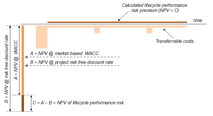
Text description of Figure 25.
Lifecycle performance risk premium calculation
This chart illustrates how the lifecycle performance risk premium can be calculated by using the difference between the market-based weighted average cost of capital (WACC) and a project risk-free discount as an indication for transferred risk.
The chart displays the transferrable costs over time, showing large capital expenses during construction, moderate O&M expenses throughout the life of the concession, and a limited number of larger expenses for major maintenance at certain points during the concession. Using arrows, the charts indicates how the transferrable costs can be discounted using a market-based WACC on the one hand, and using a project risk-free discount rate on the other. The difference is shown to be the net present value of lifecycle performance risk. The chart shows how this difference in net present value can be expressed as a flat annual risk cost over the life of the concession, which is the calculated lifecycle performance risk premium.
To calculate the lifecycle performance risk premium, both a market-based WACC and the project risk-free discount rate are required. P3-VALUE 2.2 calculates the market-based WACC from the P3 financing structure included in the model. In order to do so, the model calculates the internal rate of return of all financing cash flows combined 10, which is the project's WACC. A challenge in this approach is that the market-based WACC may also include other risks. For an availability payment (AP) project, the P3 WACC reflects the systematic risks, long-term performance risks and project coordination risks, which are mainly related to operational issues. However, the WACC for a toll concession (TC) project also reflects revenue uncertainty. P3-VALUE 2.2 therefore uses the AP WACC when calculating the lifecycle performance risk premium to ensure a fair evaluation of lifecycle performance risk in a toll concession.
In order to determine the AP WACC when evaluating a toll concession (in which case the calculated WACC by the model is the TC WACC), the model requires the user to input the difference between a TC WACC and an AP WACC. To determine what this difference in WACC should be, the user should change the active scenario in the P3-VALUE 2.2 tool (see InpFin input sheet, cell F6) from a toll concession ("PSC: Tolled, P3: Toll concession") to an AP concession ("PSC: Tolled, P3: Availability Payment"). The user must simultaneously verify that the financing conditions under the AP concession are in line with market conditions (typically higher gearing, lower DSCR and lower required equity returns for an AP transaction compared to a toll concession). Now that both the AP WACC and the TC WACC are known, the user can calculate the difference and enter the "difference between AP WACC & TC WACC" into the model (see InpFin input sheet, row 74).
The other element required to determine the lifecycle performance risk premium is the project risk-free discount rate. The project risk-free discount rate reflects the time value of money and related uncertainties and risks, just like any interest rate. The project risk-free discount rate does not reflect uncertainties and risks that are specific to a project, like an interest rate in a project finance structure for a project would. The project risk-free discount rate is a separate input that could be based on the Agency's borrowing rate (see InpFin input sheet, cell F14). Using these various elements, the model calculates the lifecycle performance risk premium, which is included as an offsetting risk cost in the PSC (and Delayed PSC) to allow for a fair comparison with the P3, both for the VfM analysis and PDBCA.
Traffic and revenues are inherently difficult to predict. In their bids for toll concessions, bidders (and their financiers) take revenue uncertainty into consideration through the financing conditions. Public Agencies that take revenue risk (under a PSC or a P3 availability payment concession) also face the same revenue uncertainty. However, it may be difficult for Agencies to value these uncertainties. P3-VALUE 2.2 allows for three different approaches to capture revenue uncertainty. Under the first approach, the user can provide a percentage reduction (an input) to toll revenues flowing to the Agency to account for uncertainty. For example, if the user inputs 20%, this means that the revenues flowing to the public Agency will be reduced by 20%. The second approach uses market-based information to determine the value of revenue uncertainty and will be discussed in more detail below. Under the third approach, the user can decide not to adjust the revenues flowing to the Agency for uncertainty.
As explained in the previous section, the difference between the AP WACC and project risk-free discount rate is a reflection of the lifecycle performance risk. Furthermore, in a toll concession, the WACC reflects both lifecycle performance risk and revenue uncertainty. P3-VALUE 2.2 uses this logic to determine the magnitude by which revenues flowing to the Agency should be reduced to account for uncertainty. To do so, the model compares the NPV of all transferrable project costs and toll revenues under 1) a market-based WACC for a toll concession and 2) a project risk-free discount rate. These NPVs are shown as D and E respectively, in Figure 26 below. The difference between the two NPVs (D - E = F) is a measure of the combined value of the lifecycle performance risk and revenue uncertainty adjustment, as illustrated in Figure 26 below.
Figure 26: Revenue Uncertainty Adjustment Calculation
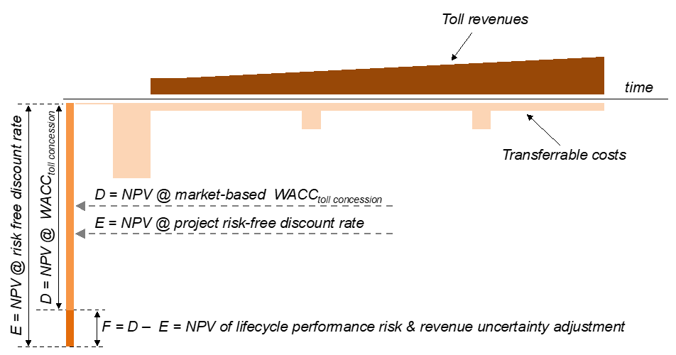
Text description of Figure 26.
Revenue uncertainty adjustment calculation
This chart illustrates how the revenue uncertainty adjustment can be calculated by using the difference between the market-based weighted average cost of capital (WACC) and a project risk-free discount as an indication for transferred risk.
The chart displays the transferrable costs over time, showing large capital expenses during construction, moderate O&M expenses throughout the life of the concession, and a limited number of larger expenses for major maintenance at certain points during the concession. It also shows the toll revenues, which are growing over time. Using arrows, the charts indicates how the transferrable costs and revenues can be discounted using a market-based WACC for a toll concession on the one hand, and using a project risk-free discount rate on the other. The difference is shown to be the net present value of the sum of the lifecycle performance risk and the revenue uncertainty adjustment.
The difference between the NPV of lifecycle performance risk (C, see Figure 25) and the NPV of the lifecycle performance risk & revenue uncertainty adjustment (F, see Figure 26) is a measure for the revenue uncertainty adjustment.
P3-VALUE 2.2 calculates the relative value of the revenue uncertainty adjustment compared to the overall revenues (in NPV terms) to determine the percentage-based reduction that should be applied to the revenues flowing to the Agency.
7 Mean = 1/2 (min + max), Variance" = 1/12 (max - min)^2
8 According to the central limit theorem, the distribution of the sum of a sufficiently large number of independent random variables is approximately normal.
9 with a and b being the minimum and maximum value respectively, and c being the most likely value (peak of the triangular probability density function).
10 Equity investment, loan/bond drawdowns, debt service, reserve movements, and dividend payments