


| AP | Availability Payment |
| BCA | Benefit Cost Analysis |
| BS | Balance Sheet |
| CF | Cash Flow |
| CFADS | Cash Flows Available to Debt Service |
| DSCR | Debt Service Coverage Ratio |
| DSRA | Debt Service Reserve Account |
| GPL | General Purpose Lanes |
| IRI | International Roughness Index |
| IRR | Internal Rate of Return |
| ML/TL | Managed Lanes or Tolled Lanes |
| MMRA | Major Maintenance Reserve Account |
| O&M | Operations and Maintenance |
| PDBCA | Project Delivery Benefit-Cost Analysis |
| P&L | Profit & Loss |
| PSC | Public Sector Comparator or Conventional Delivery |
| P3 | Public-Private Partnership |
| V/C | Volume/Capacity Ratio |
| VDF | Volume Delay Function |
| WACC | Weighted Average Cost of Capital |
This chapter provides a brief discussion of the various calculations performed in P3-VALUE 2.2. The chapter contains the following sections:
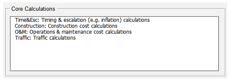
The following section presents the core calculations, which include timing and escalation, construction and O&M costs and traffic calculations. The core calculations are used in both the VfM analysis and PDBCA. In order to be able to view the sheets described in this section, please ensure you have enabled the detailed-level view in the Model Navigator. Figure 4 shows the Model Navigator's detailed-level view pane with the different calculation sheets listed.
Figure 4: Model Navigator's Detailed-level View Pane with List of Core Calculation Sheets
Core Calculations
This screenshot displays the core calculations list, including: Time and Escalation, construction cost calculations, operations and maintenance cost calculations, and traffic calculations.
This sheet calculates the various delivery models' timelines, which are shown at the top of each sheet. The sheet also contains flags and counters, which are used to simplify complex calculations. For example, a flag could indicate when the construction period ends and may be used in the subsidy calculation to ensure the subsidy is paid in the correct year. The Time&Esc sheet contains the following calculations:
This sheet calculates the pre-construction and construction costs for each delivery model. Cost items are imported from the InpTiming&Cost sheet and applied uniformly over the pre-construction and construction periods, respectively. Furthermore, indexation factors are imported from the Time&Esc sheet. Combining the various inputs and calculations, cash flows for the construction and pre-construction costs are created. Based on the calculated nominal pre-construction and construction costs, real costs for the BCA calculations are computed.
This sheet calculates the O&M and major maintenance costs for each delivery model. Cost items are imported from the InpTiming&Cost sheet whereas indexation factors are imported from the Time&Esc sheet. Combining the various inputs and calculations, cash flows for the O&M and major maintenance costs are created. Based on the calculated nominal O&M and major maintenance costs, real costs for the BCA calculations are computed.
The sheet also calculates the No Build cost savings for each delivery model. For this, annual No Build O&M costs are imported from the InpTiming&Cost sheet. The cost savings cash flows are created using the No Build O&M cost input and each delivery model's operation phase index flag from the Time&Esc sheet.
This sheet calculates traffic volumes for each year in the analysis period for both the No Build and Build. The sheet distinguishes between P50 traffic (used in the VfM analysis in combination with revenue uncertainty adjustment where appropriate) and sensitivity-adjusted traffic (used in the PDBCA module). The calculated traffic volumes are used to compute revenues, speeds, travel costs, incident delays, O&M-related travel delays, construction-related travel delays, non-fuel costs, fuel costs, accident costs, and emissions costs. The sheet uses inputs from InpTraffic&Toll, InpSeries, and Time&Esc and contains the following traffic calculations.
For a more detailed discussion on traffic projections, please refer to Part II.
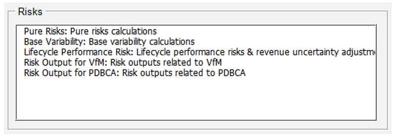
This section presents the various calculations included in the risk assessment. In order to be able to view the sheets described in this section, please ensure you have enabled the detailed-level view in the Model Navigator. Figure 5 shows the Model Navigator's detailed-level view pane with the different calculation sheets listed.
Figure 5: Model Navigator's Detailed-level View Pane with List of Calculation Sheets for Risk Assessment
Risks
This screenshot displays the risks calculations list, including: pure risks calculations, base variability calculations, lifecycle performance risks and revenue uncertainty adjustments, risk outputs related to VfM, and risk outputs related to PDBCA.
This worksheet calculates the pure risk cash flows for each delivery model. The risks are divided into construction period risks and operations period risks. The risk inputs, including the most likely risk values and other probability risk inputs, are imported from the InpRisk sheet. Indexation factors and flags are imported from the Time&Esc sheet. Using the minimum, maximum, and mean values as well as the distribution of each individual risk, the model determines the variance of each risk in order to calculate the probabilistic combined risk value in a given year based on the desired input P-level. For P3, the pure risk values are divided into retained and transferred risks, using the risk transfer percentages from the InpRisk sheet. For a more detailed discussion on pure risks, please refer to Part II.
Please note that when using the simplified inputs option, pure risks are not considered. Instead, all cost inputs must be risk- and uncertainty-adjusted.
The base variability is calculated for each delivery model to create base variability cash flows. Base variability is calculated by importing the base variability inputs for each project phase (pre-construction, construction and operations) from the InpRisk sheet and the costs from InpTiming&Cost. For P3, the base variability is divided into retained and transferred base variability, using the cost transfer percentages from the InpTiming&Cost sheet. For a more detailed discussion on base variability, please refer to Part II.
Please note that when using the simplified inputs option, base variability is not considered. Instead, all cost inputs must be risk- and uncertainty-adjusted.
The lifecycle performance risk is calculated for each delivery model to create lifecycle performance risk cash flows. The calculated lifecycle performance risk premium (option 1) is generated on this sheet using the P3 financing cost (WACC) for an availability payment concession whereas the user-specified lifecycle performance risk premium (option 2) is imported from the InpRisk sheet. The switch that determines which calculation method to use is also imported from the InpRisk sheet. Using indexation factors and phase flags from the Time&Esc sheet, the annual lifecycle performance risk premium cash flow is calculated. For a more detailed discussion on lifecycle performance risk, please refer to Part II.
The sheet also calculates a revenue uncertainty adjustment cash flow to account for uncertainty in revenues flowing to the public Agency. The calculated revenue uncertainty adjustment (option 1) is generated on this sheet using the P3 financing cost (WACC) for a toll concession whereas the user-specified risk premium input (option 2) is imported from the InpRisk sheet. The switch that determines which calculation method is also imported from the InpRisk sheet. Using indexation factors and phase flags from the Time&Esc sheet, the annual revenue uncertainty adjustment cash flow is calculated. For a more detailed discussion on revenue uncertainty adjustment, please refer to Part II.
This sheet presents the Risk output table for use in the VfM analysis.
This sheet presents the Risk output table for use in the PDBCA.
This section presents the revenue calculations, which are used in the VfM analysis. In order to be able to view the sheets described in this section, please ensure you have enabled the detailed-level view in the Model Navigator. Figure 6 shows the Model Navigator's detailed-level view pane with the calculation sheet listed.
Figure 6: Model Navigator's Detailed-view Pane with List of Revenue Calculation Sheets
Revenues
This screenshot depicts the revenues calculations title.
Revenues are calculated for tolled PSC and tolled P3 options. Revenues are not calculated for non-tolled facilities. Also, revenues are not calculated for the Delayed PSC as toll revenues are not relevant in the PDBCA module (Delayed PSC is not used in VfM). The Revenues sheet calculates three revenue cash flows: toll revenue, revenue leakage, and toll collection summary. The toll collection summary combines the first two and subtracts the revenue uncertainty adjustment calculated in the risk assessment.
Toll revenues are generated by 2 axle and 4+ axle vehicles. Their respective annual toll rates are imported from Time&Esc whereas traffic is imported from the Traffic sheet. Combining both yields the toll revenues before leakage. The toll leakage percentage is imported from the InpTraffic&Toll sheet and applied to the total toll revenue to determine the revenue leakage.
Subtracting the revenue leakage and the revenue uncertainty adjustment from the toll revenues yields the toll collection cash flow, which are used in the VfM analysis.
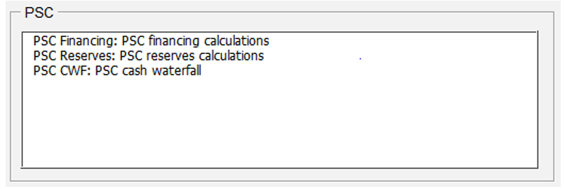
This section presents the various PSC calculations for the VfM analysis. In order to be able to view the sheets described in this section, please ensure you have enabled the detailed-level view in the Model Navigator. Figure 7 shows the Model Navigator's detailed-level view pane with the different calculation sheets listed.
Figure 7: Model Navigator's Detailed-level View With List of PSC Calculation Sheets for VfM Analysis
PSC
This screenshot lists the PSC calculations, including: PSC financing calculations, PSC reserves calculations and PSC cash waterfall.
This sheet contains the following main sections of calculations: Financing Requirements, Funding Contribution by Public Side, PSC Debt, and Debt Service Coverage Ratio (DSCR). Please note that the Model Optimizer will change some of the values on this sheet, as the macro will seek to optimize the required subsidy.
This section determines the total funding and financing requirement. To calculate this, data from several sheets is imported, including pre-construction and construction costs, and base variability and pure risks. Furthermore, issuance fees and interest during construction are brought in from further calculations on the PSC Financing sheet. Lastly, subsidies are considered to determine the total funding required during the construction period. The funding requirement is calculated using a copy-paste macro to cut circularity.
This section determines the funding contribution by the public side. In particular, it determines if the Agency needs to pre-finance any subsidy it may receive later.
This section calculates the debt drawdown, fees, interest and repayment.
For a fully sculpted loan, the repayment depends on the cash flows available for debt service (CFADS) over the entire repayment period, the outstanding balance at the start of operations, and the interest rate. Based on this, a target Debt Service Coverage Ratio (DSCR) is determined which will be applied for the entire loan repayment period. In any given year, CFADS are divided by the target DSCR to determine how much interest and principal can be paid. If the amount available to debt service falls short of the amount needed to pay interest in any given year, the interest is capitalized. As a result, the debt service profile closely follows the CFADS profile.
If an annuity-type repayment is selected, the principal repayment is determined by the debt outstanding in a given year, the number of repayment periods remaining, and the interest rate. The interest payment is based on the outstanding balance at the start of the period.
Under both PSC debt solutions, the Model Optimizer iteratively searches for a required subsidy or availability payment that results in the lowest acceptable minimum DSCR. For a more detailed discussion on the Model Optimizer, please refer to Part I 2.4.
The DSCR section calculates the yearly DSCR and the minimum DSCR. To do so, the yearly cash flow available for debt service (CFADS) is divided by the debt service cash flow to yield the yearly DSCR values. The calculated minimum DSCR value is the lowest observed value during the debt service period and will be compared against the required minimum DSCR that is provided by the user as an input.
The PSC Reserves sheet tracks the two reserve accounts: the Major Maintenance Reserve Account, and the Debt Service Reserve Account.
Every year, deposits are made into the Major Maintenance Reserve Account (MMRA) to ensure sufficient funds will be available to pay for major maintenance. The amount deposited is calculated such that by the time major maintenance is required, the amount in the MMRA is equal to the amount of the withdrawal. The anticipated amount is calculated by combining input from the O&M sheet and the Base Variability sheet. The model also considers the annual interest earned on the balance in the MMRA.
Debt service payments are imported from the PSC Financing sheet. Deposits and cash available for debt service payments are imported from the PSC CWF sheet. The previous balance, added deposits, and subtracted withdrawals result in the annual DSRA balance. Any balance in the account accrues interest.
The PSC CWF contains the high-level cash waterfall data. On this sheet, a user can see the revenues, costs, debt service, deposits and withdrawals in reserve accounts, and net cash flows. The calculations flow from top to bottom and feed directly into the next set of cash flow calculations. Cash flows are imported from the following sheets:
Together, these cash flows contribute to the calculation of:
This section presents the various P3 calculations for the VfM analysis. In order to be able to view the sheets described in this section, please ensure you have enabled the detailed-level view in the Model Navigator. Figure 8 shows the Model Navigator's detailed-level view pane with the different calculation sheets listed.
Figure 8: Model Navigator's Detailed-view Pane with List of P3 Calculation Sheets for VfM Analysis
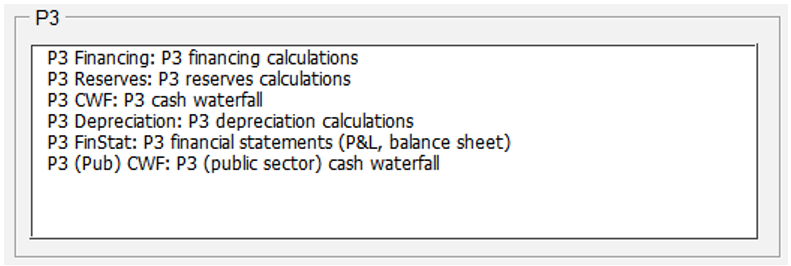
P3
This screenshot displays the P3 calculations list, including: P3 financing, P3 reserves, P3 CWF, P3 depreciation, P3 financial statements and P3 public sector cash waterfall.
This sheet contains the following main sections of calculations: Financing Requirement, Equity, Equity Bridge Loan, P3 Debt, Tax, Competitive Neutrality Adjustment, Debt Service Coverage Ratio (DSCR), and Weighted Average Cost of Capital (WACC) calculation. Please note that the Model Optimizer will change some of the values on this sheet, as the macro will seek to optimize the P3 bid.
This section determines the total funding & financing requirement. To calculate this, data from several sheets is imported, including pre-construction and construction costs, and base variability and pure risks. Furthermore, issuance fees and interest during construction are brought in from further calculations on the P3 Financing sheet. Lastly, subsidies are considered to determine the total funding required during the construction period. The funding requirement is calculated using a copy-paste macro to cut circularity.
In this section, the amount of equity injection is determined. The calculated funding requirement is used in conjunction with the gearing ratio to determine how much equity is required.
In this section, the equity bridge loan drawdown and repayment is calculated. The equity bridge loan is used to provide short-term financing that will be taken out by government subsidy, and not included in the debt portion of the gearing ratio.
This section calculates the debt drawdown, fees, interest, and repayment.
For a fully sculpted loan, the repayment depends on the cash flows available for debt service (CFADS) over the entire repayment period, the outstanding balance at the start of operations, and the interest rate. Based on this, a target Debt Service Coverage Ratio (DSCR) is determined which will be applied for the entire loan repayment period. In any given year, CFADS are divided by the target DSCR to determine how much interest and principal can be paid. If the amount available to debt service falls short of the amount needed to pay interest in any given year, the interest is capitalized. As a result, the debt service profile closely follows the CFADS profile.
If an annuity-type repayment is selected, the principal repayment is determined by the debt outstanding in a given year, the number of repayment periods remaining, and the interest rate. The interest payment is based on the outstanding balance at the start of the period.
Under both P3 debt solutions, the Model Optimizer iteratively searches for a required subsidy or availability payment that results in the lowest acceptable minimum DSCR while still satisfying the equity return requirement. For a more detailed discussion on the Model Optimizer, please refer to Part I 2.4.
To determine how much tax needs to be paid by the P3 concessionaire in a given year, income profits and losses are tracked. This sheet tracks all profits, losses, and losses carried forward to determine the annual taxable profits. Federal and state taxes are then calculated based on the taxable profits.
Based on the federal and state tax liability, self-insurance inputs, and credit subsidies inputs, the model calculates the competitive neutrality adjustment for each of these items.
The DSCR section calculates the yearly DSCR and the minimum DSCR. To do so, the yearly cash flow available for debt service (CFADS) is divided by the debt service cash flow to yield the yearly DSCR values. The calculated minimum DSCR value is the lowest observed value during the debt service period and will be compared against the required minimum DSCR that is provided by the user as an input.
The lifecycle performance risk premium calculation and revenue uncertainty adjustment requires the P3 Weighted Average Cost of Capital (WACC). This section brings together all relevant financing cash flows to determine the project's effective WACC.
The P3 Reserves sheet tracks the two reserve accounts: The Major Maintenance Reserve Account, and the Debt Service Reserve Account.
Every year, deposits are made into the Major Maintenance Reserve Account (MMRA) to ensure sufficient funds will be available to pay for major maintenance. The amount deposited is calculated such that by the time major maintenance is required, the amount in the MMRA is equal to the amount of the withdrawal. The anticipated amount is calculated by combining input from the O&M sheet and the Base Variability sheet. The model also considers the annual interest earned on the balance in the MMRA.
Debt service payments are imported from the P3 Financing sheet. Deposits and cash available for debt service payments are imported from the P3 CWF sheet. The previous balance, added deposits, and subtracted withdrawals result in the annual DSRA balance. Any balance in the account accrues interest.
The P3 CWF contains the high-level cash waterfall data. On this sheet, a user can see the revenues, costs, debt service, movements in reserve accounts, and net cash flows. The calculations flow from top to bottom and feed directly into the next set of cash flow calculations. Cash flows are imported from the following sheets:
Together, these cash flows contribute to the calculation of:
The P3 Depreciation sheet tracks two major assets: Fixed Asset and Major Maintenance Asset.
The model adds construction costs, pure construction risks, construction base variability costs, capitalized interest and debt fees during the construction phase to the fixed asset balance. Depreciation is calculated based on the remaining depreciation period and subtracted from the balance.
Expenses on major maintenance are added to the Major Maintenance Asset balance. Depreciation is calculated using a Major Maintenance Asset depreciation rate, which is based off the major maintenance periodicity.
This sheet contains two financial statements: The Income Statement and the Balance Sheet. The income statement calculates the annual operating profit, profit before interest and tax, profit before tax, profit after tax / net cash flow, and retained earnings. The balance sheet calculates for each year the project's assets and liabilities.
This sheet tracks the cash waterfall from the public Agency's point of view. Toll revenues for the public side are imported from the Revenues sheet. Any availability payments made are imported from the Subsidy & Bid sheet. Retained operations and maintenance costs, as well as the base variability of those costs, are imported from the O&M sheet and the Base Variability sheet. Retained construction costs are imported from the Construction sheet. Together, these cash flows are used to create the P3 (Public) net cash flows and retained cash balance.
This section presents the VfM calculations performed to compare P3 and PSC project delivery. In order to be able to view the sheets described in this section, please ensure you have enabled the detailed-level view in the Model Navigator. Figure 9 shows the Model Navigator's detailed-level view pane with the different calculation sheets listed.
Figure 9: Model Navigator's Detailed-level View Pane with List of VfM Calculation Sheets
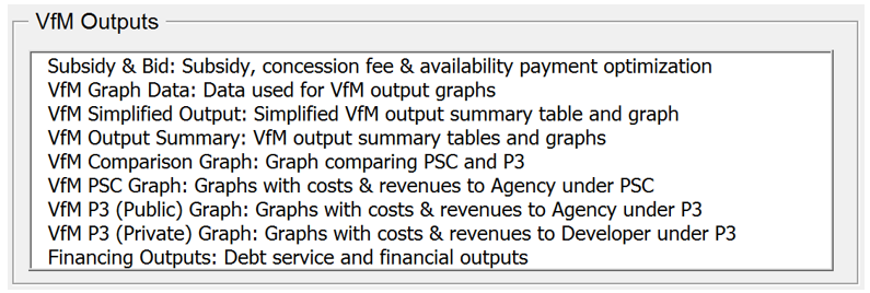
VfM Outputs
This screenshot displays a list of VfM outputs, including: Subsidy and bid, VfM Graph data, VfM simplified output, VfM output summary, VfM comparison graph, VfM PSC graph, VfM P3 public graph, VfM private graph, and financing outputs.
This sheet calculates the required PSC subsidy and the required P3 subsidy or availability payment. The sheet uses macros to determine the lowest acceptable subsidy/availability payment. The sheet contains the following elements:
This sheet calculates the net present values of costs and revenues and contains data used in the various output tables and graphs.
This sheet presents a simplified VfM output summary table and graph.
This sheet presents VfM output summary tables and graphs.
This sheet presents the VfM graph comparing PSC and P3.
This sheet presents graphs with costs and revenues to the Agency under a PSC.
This sheet presents graphs with costs and revenue to the agency under a P3.
This sheet presents graphs with costs and revenue to the developer (i.e., concessionaire) under a P3
This sheet presents debt service and financial outputs.
This section presents the travel cost calculations. In order to be able to view the sheets described in this section, please ensure you have enabled the detailed-level view in the Model Navigator. Figure 10 shows the Model Navigator's detailed-level view pane with the different calculation sheets listed.
Figure 10: Model Navigator's Detailed-level View Pane with List of Calculation Sheets for Travel Costs
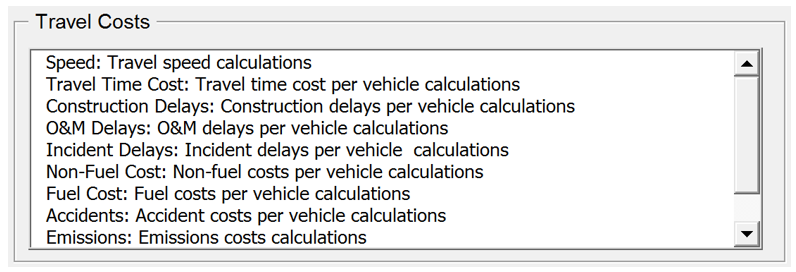
Text description of Figure 10.
Travel Costs
This screenshot displays a listing of travel costs calculations, including: Speed, travel time cost, construction delays, O&M delays, incident delays, non-fuel cost, fuel cost, accidents, and emissions.
This sheet calculates speeds for each year in the analysis period for the various delivery models. These speeds are used to compute travel time costs, incident delays, O&M-related travel delays, construction-related travel delays, non-fuel costs, fuel costs, and emissions costs. The following presents the order of calculations in this sheet.
This sheet calculates travel time costs for each year in the analysis period for the various delivery models. These travel time costs are also used to compute construction and O&M-related travel delays and incident delays.
No Build and Build (ML/TL and GPL) travel time costs for peak, off-peak, and weekends are calculated using segment length from the InpTraffic&Toll sheet, vehicle occupancy and value of time inputs from the InpBCA sheet, operations flags from the InpSeries sheet, and congested speeds from the Speed sheet. The calculations of congested travel time costs are performed separately for 2 axle and 4+ axle vehicles. For a more detailed discussion on calculation of travel time costs, please refer to Part II.
This sheet calculates construction-related travel delay costs for each year in the analysis period for the various delivery models. No Build and Build (ML/TL and GPL) construction-related travel delay costs for peak, off-peak, and weekends for 2 and 4+ axle vehicles are calculated using input parameters from the various input sheets and travel time costs from the Travel Time Costs sheet. For a more detailed discussion on calculation of construction-related delays, please refer to Part II.
This sheet calculates O&M-related travel delay costs for each year in the analysis period for the various delivery models. No Build and Build (ML/TL and GPL) O&M-related travel delay costs for peak, off-peak, and weekends for 2 and 4+ axle vehicles are calculated using input parameters from the various input sheets and travel time costs from the Travel Time Costs sheet. This sheet borrows calculations performed in the Construction Delays sheet so as to not repeat some of the calculations. For a more detailed discussion on calculation of O&M-related travel delays, please refer to Part II.
This sheet calculates incident delay costs for each year in the analysis period for the various delivery models. No Build and Build (ML/TL and GPL) incident delay costs for peak, off-peak, and weekends for 2 and 4+ axle vehicles are calculated using speed adjustment factors from the BCA input sheets and travel time costs from the Travel Time Costs sheet. For a more detailed discussion on calculation of incident delays, please refer to Part II.
This sheet calculates non-fuel costs for each year in the analysis period for the various delivery models. No Build and Build (ML/TL and GPL) non-fuel costs for peak, off-peak, and weekends for 2 and 4+ axle vehicles are calculated using input parameters from the various input sheets. These calculations incorporate pavement quality adjustments. For a more detailed discussion on calculation of non-fuel costs, please refer to Part II.
This sheet calculates fuel costs for each year in the analysis period for the various delivery models. No Build and Build (ML/TL and GPL) fuel costs for peak, off-peak, and weekends for 2 and 4+ axle vehicles are calculated using input parameters from the various input sheets. These calculations incorporate pavement quality adjustments. For a more detailed discussion on calculation of fuel costs, please refer to Part II.
This sheet calculates accident costs for each year in the analysis period for the various delivery models. No Build and Build (ML/TL and GPL) accident costs for peak, off-peak, and weekends for 2 and 4+ axle vehicles are calculated using input parameters from the various input sheets. For a more detailed discussion on calculation of accident costs, please refer to Part II.
This sheet calculates emissions costs for each year in the analysis period for the various delivery models. No Build and Build (ML/TL and GPL) emissions costs for peak, off-peak, and weekends for 2 and 4+ axle vehicles are calculated using input parameters from the various input sheets as well as traffic projections from the Traffic sheet. For a more detailed discussion on calculation of emission costs, please refer to Part II.
This sheet calculates transit passenger volumes for each year in the analysis period for both the No Build and Build. The sheet effectively mirrors large sections of the "Traffic" worksheet, using an identical input structure and largely following the same calculation logic.
This sheet calculates carpooling passenger volumes for each year in the analysis period for both the No Build and Build. The sheet effectively mirrors large sections of the "Traffic" worksheet, using an identical input structure and largely following the same calculation logic.
This section presents the benefits calculations. In order to be able to view the sheets described in this section, please ensure you have enabled the detailed-level view in the Model Navigator. Figure 11 shows the Model Navigator's detailed-level view pane with the different calculation sheets listed.
Figure 11: Model Navigator's Detailed-level View Pane with List of Benefits Calculation Sheets
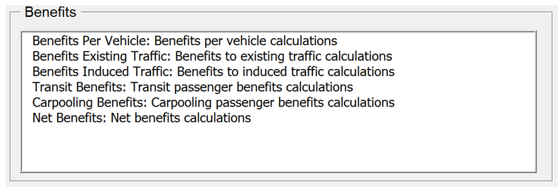
Text description of Figure 11.
Benefits
This screenshot displays a list of benefits calculations, including: benefits per vehicle, benefits existing traffic, benefits induced traffic, transit benefits, carpooling benefits, and net benefits.
This sheet calculates benefits per vehicle for the PSC, Delayed PSC, and P3 by subtracting the No Build cost per vehicle from the Build cost per vehicle for each year in the analysis period. The following benefits per vehicle are calculated in this sheet:
This sheet calculates benefits for existing traffic for the PSC, Delayed PSC, and P3 by multiplying the benefits per vehicle for each benefit type by the existing traffic for each year in the analysis period. The following benefits are calculated in this sheet:
This sheet calculates benefits for induced traffic for the PSC, Delayed PSC, and P3. Induced traffic benefits consist of a consumer surplus and a producer surplus. To calculate the consumer surplus, the induced traffic is multiplied by half the difference in user costs between the No Build and Build. This "rule of half" (see Part II for a discussion on the "rule of half") is applied to capture the triangular shape of the consumer surplus, i.e., the triangle under the demand curve that corresponds to the induced traffic created by the shift in supply due to the road expansion. The user costs include:
To calculate the producer surplus, the induced traffic is multiplied by the Build toll. The induced traffic benefits equal the sum of consumer and producer surplus. The induced traffic benefits are subsequently allocated to the different benefit categories, using the existing traffic benefit split. For a more detailed discussion on calculation of induced traffic benefits, please refer to Part II.
This sheet calculates the travel time cost savings for existing transit passengers under each delivery model, using the calculated travel time savings for 4+ axle vehicles. Based on the travel time cost savings for existing transit passengers, the model calculates the societal benefits for induced transit passengers using the "rule of half" in order to determine the total transit passenger benefits under each delivery model.
This sheet calculates the travel time cost savings for existing carpooling passengers under each delivery model, using the calculated travel time savings for 2 axle vehicles. Based on the travel time cost savings for existing carpooling passengers, the model calculates the societal benefits for induced carpooling passengers using the "rule of half" in order to determine the total carpooling passenger benefits under each delivery model.
This sheet calculates the net benefits for each year in the analysis period for the PSC, Delayed PSC, and P3 compared to the No Build. The following presents the order of calculations in this sheet.
This section presents the PDBCA calculations performed to compare P3, PSC, and Delayed PSC project delivery. In order to be able to view the sheets described in this section, please ensure you have enabled the detailed-level view in the Model Navigator. Figure 12 shows the Model Navigator's detailed-level view pane with the different calculation sheets listed.
Figure 12: Model Navigator's Detailed-level View Pane with List of PDBCA Calculation Sheets
Text description of Figure 12.
PDBCA Outputs
This screenshot lists calculations for the PDBCA outputs, including: PDBCA graph data, PDBCA output summary, PDBCA incremental comparison, PDBCA delayed PSC graph, PDBCA PSC graph, and PDBCA P3 graph.
This sheet calculates the net present values of costs and benefits and contains data used in the various output tables and graphs.
This sheet presents PDBCA output summary tables and graphs.
This sheet presents tables and a graph comparing Delayed PSC, PSC, and P3.
This sheet presents graphs with costs and benefits to society under Delayed PSC.
This sheet presents graphs with costs and benefits to society under PSC.
This sheet presents graphs with costs and benefits to society under P3.