


| AP | Availability Payment |
| BCA | Benefit Cost Analysis |
| BS | Balance Sheet |
| CF | Cash Flow |
| CFADS | Cash Flows Available to Debt Service |
| DSCR | Debt Service Coverage Ratio |
| DSRA | Debt Service Reserve Account |
| GPL | General Purpose Lanes |
| IRI | International Roughness Index |
| IRR | Internal Rate of Return |
| ML/TL | Managed Lanes or Tolled Lanes |
| MMRA | Major Maintenance Reserve Account |
| O&M | Operations and Maintenance |
| PDBCA | Project Delivery Benefit-Cost Analysis |
| P&L | Profit & Loss |
| PSC | Public Sector Comparator or Conventional Delivery |
| P3 | Public-Private Partnership |
| V/C | Volume/Capacity Ratio |
| VDF | Volume Delay Function |
| WACC | Weighted Average Cost of Capital |
To develop the PDBCA framework and the P3-VALUE 2.2 PDBCA module, a number of concepts were developed while other existing concepts were adapted to the new framework. Furthermore, in order to be able to compare different delivery models, the PDBCA module required a calculation methodology for each potential benefit (or disbenefit) considered. This chapter discusses a number of the key concepts and describes the calculation methodology for the various benefits considered in the PDBCA framework, including:
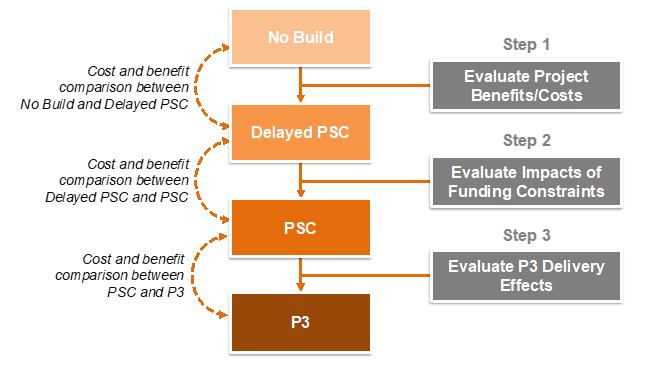
In the VfM analysis, the PSC is compared to the P3 in order to determine the fiscal impact on the Agency of P3 procurement. A key requirement for a VfM analysis to be valid is that the PSC and the P3 are implemented in a similar timeframe. For the PDBCA, there is no such requirement. Under PDBCA, a delayed project can be compared to an accelerated project without any conceptual challenges. This means that the PDBCA framework allows practitioners to evaluate the impact of funding constraints that could delay projects. As shown in Figure 29 below, P3-VALUE 2.2 uses three steps to distinguish between the impacts of public funding constraints on the one hand, and impacts due to P3 cost and benefit efficiencies on the other.
Figure 29: PDBCA Framework
Text description of Figure 29.
This model shows the process for comparing different scenarios for funding. The scenarios compared are no build, delayed PSC, PSC, and P3. These are set in relation to three steps of project analysis: Step 1 (evaluate project benefits/costs), step 2 (evaluate impacts of funding constraints), and step 3 (evaluate P3 delivery effects). The diagram also shows comparison between each of the successive scenarios (BCA between No build and delayed PSC, BCA between delayed PSC and PSC, and BCA between PSC and P3).
To evaluate the impacts of funding constraints (step 2 in the figure above), a third delivery model is therefore introduced: The Delayed Public Sector Comparator (Delayed PSC).
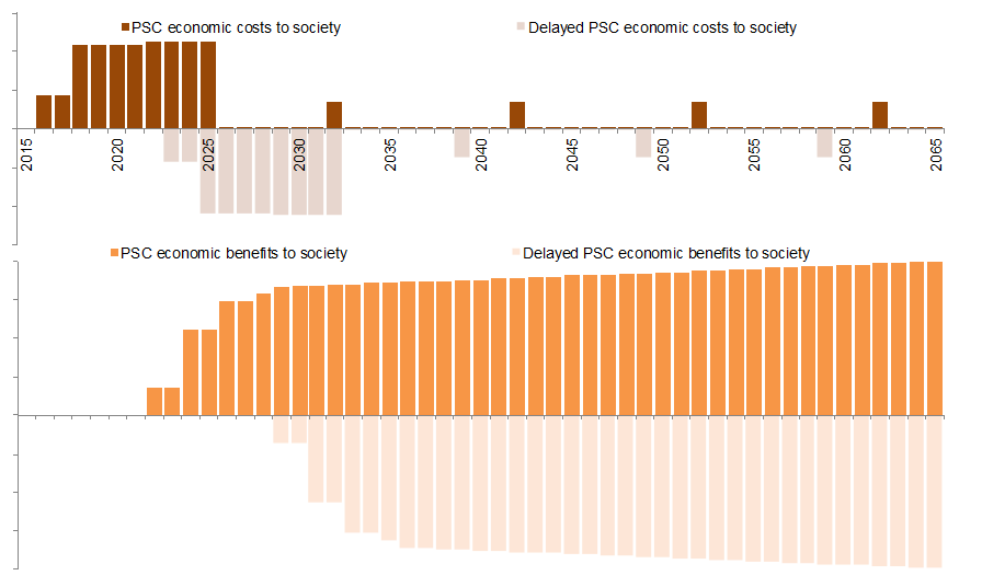
The Delayed PSC has the exact same characteristics as the PSC, with only one exception: the start date of the project. If, for example, due to fiscal constraints an Agency can only afford to start building a project in 2025 instead of 2018, both the incurred costs as well as the benefits accruing to society will be delayed. Figure 30 below shows the impact of such delay on both the economic costs and benefits to society. As can be seen from the figure, both the cost and benefits are delayed by the same number of years (7 in the example shown below).
Figure 30: Comparison of Economic Costs & Benefits Between Delayed PSC and PSC
Text description of Figure 30.
Comparison of economic costs and benefits between PSC and Delayed PSC
This figure shows a histogram that compares annual economic costs and benefits under the PSC to annual economic costs and benefits under the delayed PSC. It demonstrates that the delayed PSC differs from the PSC only in the timing of costs and benefits.
Depending on the exact profile of costs and benefits, accelerating a project may result in lower or higher net benefits to society.
Value of Time (VOT) reflects the economic value of time spent by travelers on their journey. The P3-VALUE 2.2 tool uses VOT to calculate differences in travel time cost (i.e., travel time cost savings) between the No Build and various Build options (Delayed PSC, PSC, and P3). VOT is typically not project-specific but may vary by region. For example, a region with a high median income is expected to have a higher VOT when compared to a region with a low median income.
The P3-VALUE 2.2 tool enables users to evaluate a variety of highway projects, including projects with general purpose lanes (GPL) and/or tolled lanes/managed lanes (TL/ML). For a managed lanes project, users of the facility have a choice between taking the GPL and not paying a toll vs. paying a toll to access the ML in order to enjoy greater travel time savings. Typically, people willing to pay tolls tend to value their time at a higher rate. Therefore, VOT is expected to be higher for ML users. As the overall average VOT for the Build and No Build alternative should be equal, VOT of the GPL users could theoretically be determined from the relative traffic shares on the MLs and GPLs (in combination with the VOT of the No Build and the ML users). Given the already significant complexity of the traffic calculations 11 in P3-VALUE 2.2, P3-VALUE applies a uniform VOT to GPL and ML/TL users.
Traffic plays an important role in the PDBCA module as the various benefits and disbenefits are directly related to the number of users on the facility. To determine traffic on the facility, P3-VALUE 2.2 requires users to provide average weekday daily traffic (AWDT). More specifically, the user must provide a most likely traffic projection (P50 equivalent) by inputting a minimum of two (but up to five) traffic data points (traffic in a specified year). The tool uses a simple straight line interpolation for the intermediate years. Beyond the last year of input, the tool uses a constant growth factor (input provided by user) to project future traffic.
To avoid unrealistically high traffic projections, the model automatically limits overall daily traffic to the following daily capacity (maximum number of vehicles that can use the facility per day):
Daily capacity = hourly-to-daily capacity conversion factor x ratio of LOS E capacity to LOS C capacity x lane vehicle capacity at LOS C x number of lanes
The hourly-to-daily capacity conversion factor is defined as the ratio of the maximum daily traffic divided by the level of service (LOS E) hourly capacity. The LOS E to LOS C capacity ratio is defined as the ratio of the vehicle service volume at LOS E divided by the vehicle service volume at LOS C, i.e., the service volume used in the volume-delay function (VDF) used to calculate congested speeds, which is discussed below. The variables in the above formula are all user inputs. For example, if the hourly-to-daily capacity conversion factor is 12, in combination with a LOS E to LOS C capacity ratio of 1.33 12, lane vehicle capacity at LOS C of 1,500 vehicles per lane per hour and 6 lanes, the maximum traffic accepted by the model is 143,640 vehicles per day.
If the user-generated daily traffic inputs or model forecasts based on input growth rates exceeds the facility's maximum daily capacity, the model cuts off any excess traffic and informs the user through alerts that the traffic capacity has been breached. In that case, the capped maximum daily capacity is used to calculate the various traffic streams (peak vs. off-peak, weekday vs. weekend, 2 axles vs. 4+ axles traffic). The maximum daily capacity also constrains the traffic projections used for the toll revenue calculation in the VfM analysis.
One of the key benefits of a highway expansion project is likely to be the reduction of travel time cost (or travel time savings) for its users. To determine the travel time savings to users, P3-VALUE 2.2 calculates the travel time under the different delivery models and compares it to the No Build travel times. To determine the travel times, the model calculates the actual congested speeds due to recurring congestion under the traffic projections provided.
Congested speeds due to recurring congestion are computed for each of the delivery models using each year's traffic volume and capacity by period. The cost of travel is calculated by multiplying the congested travel time by the value of time (input). The travel time cost difference between the various delivery models considered and the No Build is the travel time benefit. The rest of this section details how congested speeds and travel time costs are computed.
P3-VALUE 2.2 calculates congested speeds due to recurring congestion for each year and delivery model considered, for the different portions of the facility (GPL and ML/TL), for each vehicle type (2 and 4+ axle), and for each time period (peak, off-peak, and weekend) using the Bureau of Public Roads' Volume-Delay Function (VDF):
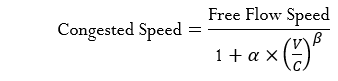
While the form of the VDF function cannot be changed within the tool, the parameters (α and β) can be changed by the user. The default value for α is 0.15 and β is 4. The user can modify these parameters to calibrate congested speeds to observed congested speeds for the existing facility. The capacity used in the formula is the hourly capacity at Level of Service C (LOS C capacity), not the maximum hourly capacity (LOS E capacity). Thus, a freeway lane with an LOS E capacity of 2,000 vehicles per lane per hour would have a LOS C capacity of approximately 1,500 vehicles per lane per hour, resulting in the 1.33 LOS E vehicle-capacity factor used on the previous page. In order to obtain accurate speeds, it is important to use the LOS C capacity as input. Using LOS E capacity as input would cause an underestimation of congested speeds, and result in an underestimation of benefits from increasing capacity. If the user inputs traffic volumes and VDF parameters from a well-calibrated and validated travel demand model, the congested travel speeds on the existing facility should be comparable to the observed travel speeds. If the user does not have access to a calibrated travel demand model, then the user may seek assistance from a travel demand modeler to help calibrate the VDF parameters.
P3-VALUE 2.2 computes travel time costs for every year in the analysis period for the No Build and each of the delivery models considered. The model uses the following formulae to calculate the travel time cost for each period (peak, off-peak, and weekend), vehicle type, and lane type (GPL and ML/TL):
![Travel Time Cost/Vehicle = Vehicle Occupancy x Value of Time x Project Length / Congested Speed Travel Time Cost Savings/Vehicle = [( Travel Time Cost/Vehicle )] / Build [(- Travel Time Cost/Vehicle )] / No Build Travel Time Cost Savings = Travel Time Cost Savings/Vehicle x Existing Traffic](/ipd/images/p3/toolkit/p3_value_2_2/2_6_formula_3.png)
The model calculates and compares the travel time costs of the various Build delivery models with the travel time costs of the No Build to determine the travel time cost savings per vehicle for each delivery model. The total travel time benefit is the travel time cost savings per vehicle multiplied by the existing traffic volume (i.e., the No Build traffic volume, which excludes induced traffic, see below).
P3-VALUE 2.2 also considers the social impact of delays due to lane unavailability during construction as well as operations and maintenance (O&M). The model uses the following formula to calculate the delay cost per vehicle.
![Delay Cost/Vehicle = Travel Time Cost/Vehicle x [1/(1- Speed Adjustment Factor) - 1)]](/ipd/images/p3/toolkit/p3_value_2_2/2_6_formula_4.png)
The right part of the equation above represents the increase in travel time (and therefore travel time cost) of a reduction in speed. For example, if a user usually travels at 50 miles per hour, he/she will take 24 minutes to cover a road segment of 20 miles. If his/her speed is reduced by 20% to 40 miles per hour, he will now take 30 minutes to cover the same distance. This is equal to a 25% increase in travel time and travel time cost. The right part of the formula calculates this percentage increase in travel time cost.
Using the above, the model uses the following formulae to calculate the social cost of delays for each delivery model, period (peak, off-peak, and weekend), vehicle type, and lane type (GPL and ML/TL
![â–³Delay Cost/Vehicle =[( Delay Cost/Vehicle )] / Build -[( Delay Cost/Vehicle )] / No Build
Traffic Affected (%) =( Construction days/O&M days per year x Delay Duration )/ Hours in a year
Segment Affected (%) = Length of Affected Segment / Total Segment Length
Annual Delay Cost = Traffic Affected x Segment Affected x â–³Delay Cost/Vehicle x Existing Traffic](/ipd/images/p3/toolkit/p3_value_2_2/2_6_formula_5.png)
The model calculates and compares the delay costs of the various Build delivery models with the delay costs of the No Build to determine the change in delay costs per vehicle for each delivery model. Based on the share of traffic affected, the length of the section of the facility affected, the calculated change in delay costs and the existing traffic, the model calculates the annual delay costs for each of the delivery models.
A key input for the delay calculation is the speed adjustment factor, which determines by how much speed is adjusted based on number of lanes that are open. For work zones, this speed adjustment is to a large extent due to the lower posted speed limits that require vehicles to slow down. Table 17 presents speed adjustment factors for work zones. Based on the number of open lanes and the free flow speed, the table provides a speed adjustment factor. The shaded cells in the table (ranging from 0.52 to 0.57) present the most common situation for work zones on highways. P3-VALUE 2.2 uses the average of the highlighted cells as a default value (0.55, or a 45% speed reduction), but users may modify this input to better fit regional conditions.
Table 17: Speed Adjustment Factors for Work Zones (Construction and O&M Delays)
| Lanes Open | 55 mph | 60 mph | 65 mph | 70 mph | 75 mph |
|---|---|---|---|---|---|
| 1 | 0.60 | 0.56 | 0.53 | 0.50 | 0.47 |
| 2 | 0.62 | 0.58 | 0.55 | 0.52 | 0.49 |
| 3 | 0.64 | 0.60 | 0.57 | 0.54 | 0.51 |
| 4 | 0.66 | 0.62 | 0.58 | 0.55 | 0.52 |
| 5 | 0.68 | 0.64 | 0.60 | 0.57 | 0.53 |
Source: Table G.9. Capacity and Minimum Free-Flow Speed Adjustment Factors for Work Zones from SHRP 2 Project L08, Freeways (http://www.trb.org/Publications/Blurbs/169594.aspx)
As explained above, P3-VALUE 2.2 determines the additional travel time cost due to construction and O&M delays. These include delays in work zones due to speed reductions but exclude any additional queuing delays. As construction and O&M activities are usually carried out during off-peak hours and weekends, queuing will typically be limited. To capture the effects of queuing, users may choose to input a speed reduction factor based on regional observations and/or modify the affected segment length. The model does not calculate the change in vehicle operating, accidents and emission costs caused by these travel delays. Instead, the model uses average annual (congested) speeds to calculate these costs for the different vehicle types and periods (peak, off-peak, and weekend) as will be discussed below.
Besides delays due to construction and O&M activities, P3-VALUE 2.2 also considers the travel cost impact of delays due to incidents. The model uses the following formula to calculate the delay cost per vehicle due to incidents.
![Incident Delay Cost/Vehicle = Travel Time Cost/Vehicle x [1/(1- Speed Adjustment Factor) -1]](/ipd/images/p3/toolkit/p3_value_2_2/2_6_formula_6.png)
The right part of the equation above represents the increase in travel time (and therefore travel time cost) of a reduction in expected average speed for all vehicles when the probability of incidents (throughout the year) is taken into consideration. It should be noted that the speed adjustment represents an average for the whole year. On days that incidents do occur, the actual average speed would of course be much lower (and delays higher), while on days when no incidents occur the actual speeds would be higher (and delays lower). An important difference with the calculation of delays due to construction and O&M is therefore that the average speed adjustment related to incidents is applied to all traffic on the entire highway facility being analyzed.
The model uses the following process to calculate the social cost of delays for each delivery model, period (peak, off-peak, and weekend), vehicle type, and lane type (GPL and ML/TL):
![â–³Incident Delay Cost/Vehicle = Incident [( Delay Cost/Vehicle )] / Build -[( Incident Delay Cost/Vehicle )]_ / No Build
Annual Incident Delay Cost = â–³Incident Delay Cost/Vehicle x Existing Traffic](/ipd/images/p3/toolkit/p3_value_2_2/2_6_formula_7.png)
The model calculates and compares the incident delay costs of the various Build delivery models with the incident delay costs of the No Build to determine the change in incident delay costs per vehicle for each delivery model.
A key input for the incident delay calculation is the speed adjustment factor, which determines by how much average (congested) speed is adjusted to account for incident delays. For incidents, this speed adjustment is to a large extent due to queuing that occurs as a result of capacity reduction. Table 18 presents the speed adjustment factors for various levels of recurring congestion severity, based on data from unpublished estimates of average speed by level of congestion for Los Angeles area freeways 13. The P3-VALUE 2.2 user may use this table, along with information about the level of congestion severity under the No Build, Build PSC and Build P3 scenarios respectively to derive an appropriate speed adjustment factor. Please note that P3-VALUE 2.2 assumes the speed adjustment factor to be constant over time.
Table 18: Speed Adjustment Factors for Incidents (Based on TTI Data)
| Level of congestion | Speed with no incidents (avg mph) | Speed including incidents (avg mph) | Speed adjustment factor (% reduction in speed) |
| Uncongested | 60.0 | 57.1 | 5% |
| Medium | 55.7 | 53.0 | 5% |
| Heavy | 51.4 | 46.7 | 9% |
| Severe | 41.5 | 34.1 | 18% |
| Extreme | 35.0 | 27.1 | 23% |
Besides the travel time costs discussed above, the model also considers other service quality effects. One of these service quality effects could be a different pavement ride quality under a P3. P3-VALUE 2.2 allows users to specify as inputs the pavement ride quality under different delivery models.
Better pavement ride quality could potentially have the following impacts:
In practice, the impact of pavement ride quality on speed is not significant. If the Pavement Smoothness Index (PSI) exceeds 2.5, there is no impact on speed 14. Below that, there is a limited impact on speeds. Given that pavement quality on U.S. highways tends to be well above a PSI of 2.5, P3-VALUE 2.2 does not adjust speeds for pavement quality. Pavement quality does have an impact on fuel and non-fuel vehicle operating costs, which will be discussed below.
P3-VALUE 2.2 computes fuel costs for each year within the analysis period. For each delivery model, period (peak, off-peak, and weekend), vehicle type, and lane type (GPL and ML/TL), the tool takes into consideration the impact of pavement ride quality on fuel cost. The model uses the following formulae to calculate these costs:
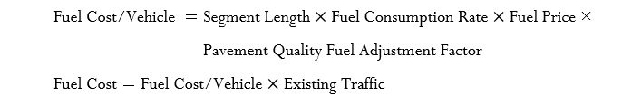
Fuel costs per vehicle are computed by multiplying the segment length, fuel consumption rate, fuel price and the pavement ride quality fuel consumption adjustment factor. Total fuel costs are calculated by multiplying existing traffic by the fuel cost per vehicle.
As fuel consumption rates vary by speed of travel, the tool looks up the fuel consumption rate based on the average speed for each delivery mode, period, vehicle type, and lane type. P3-VALUE 2.2 provides default values for the speed-adjusted fuel consumption rates, but users are free to change these. Furthermore, the tool applies a pavement quality fuel consumption adjustment factor based on the delivery model's International Roughness Index (IRI). Table 19 presents the default inputs for the pavement quality fuel consumption adjustment factor.
Table 19: Pavement Quality Fuel Consumption Adjustment Factors
| IRI | Auto | Truck |
|---|---|---|
| 0 | 0.97 | 0.96 |
| 25 | 0.98 | 0.97 |
| 50 | 0.98 | 0.97 |
| 75 | 0.98 | 0.98 |
| 100 | 0.98 | 0.98 |
| 125 | 0.99 | 0.99 |
| 150 | 1.00 | 0.99 |
| 175 | 1.00 | 1.00 |
| 200 | 1.01 | 1.01 |
| 225 | 1.01 | 1.02 |
| 250 | 1.02 | 1.03 |
| 275 | 1.03 | 1.04 |
| 300 | 1.03 | 1.05 |
| 325 | 1.04 | 1.06 |
| 350 | 1.05 | 1.07 |
| 375 | 1.06 | 1.08 |
| 400 | 1.07 | 1.10 |
| 425 | 1.08 | 1.11 |
| 450 | 1.09 | 1.13 |
Source: Surface Characteristics of Roadways: International Research and Technologies (1990) and Vehicle-Road Interaction (1994)
P3-VALUE 2.2 also calculates non-fuel vehicle operating for each year within the analysis period. For each delivery model, period (peak, off-peak, and weekend), vehicle type, and lane type (GPL and ML/TL), the tool takes into consideration the impact of pavement ride quality on non-fuel vehicle operating cost. The model uses the following formulae to calculate these costs:
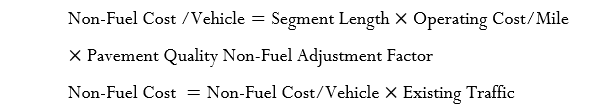
Non-fuel costs per vehicle are computed by multiplying the segment length and the cost per mile. To adjust for the effects of the pavement quality, a pavement quality non-fuel vehicle operating cost adjustment factor is applied based on the delivery model's International Roughness Index (IRI). Table 20 presents the default inputs for this adjustment factor. Total non-fuel costs are calculated by multiplying existing traffic by the non-fuel cost per vehicle.
Table 20: Pavement Quality Non-Fuel Vehicle Operating Cost Adjustment
| IRI | Auto | Truck |
|---|---|---|
| 0 | 1.00 | 1.00 |
| 25 | 1.00 | 1.00 |
| 50 | 1.00 | 1.00 |
| 75 | 1.00 | 1.00 |
| 100 | 1.00 | 1.00 |
| 125 | 1.00 | 1.00 |
| 150 | 1.02 | 1.02 |
| 175 | 1.03 | 1.04 |
| 200 | 1.05 | 1.06 |
| 225 | 1.07 | 1.08 |
| 250 | 1.09 | 1.10 |
| 275 | 1.11 | 1.12 |
| 300 | 1.12 | 1.14 |
| 325 | 1.14 | 1.16 |
| 350 | 1.16 | 1.18 |
| 375 | 1.18 | 1.20 |
| 400 | 1.19 | 1.22 |
| 425 | 1.21 | 1.24 |
| 450 | 1.23 | 1.26 |
Source: ARRB Research Board TR VOC Model (NCHRP Report 720: Estimating the Effects of Pavement Condition on Vehicle Operating Costs)
Another potential difference between delivery models could be the societal cost of accidents. P3-VALUE 2.2 calculates these costs for each delivery model, period (peak, off-peak, and weekend), vehicle type, and lane type (GPL and ML/TL). The model uses the following formulae to calculate the social costs of accidents:
Accident costs per vehicle are computed by multiplying the segment length, accident rate per mile, and cost per accident. Total accident costs are calculated by multiplying accident costs per vehicle by existing traffic.
Based on their features, accident rates may vary between different delivery models. Users of P3-VALUE 2.2 will have to determine whether and to what extent accident rates vary between different delivery models. The table below presents accident rates from the National Highway Traffic Safety Administration (NHTSA), which may be used as default values in the model.
Table 21: Accident Rates
| Accident Type | Rate (accident/million VMT) |
|---|---|
| Fatal accidents | 0.0109 |
| Injury accidents | 0.7700 |
| Property damage only accidents | 1.9000 |
Source: NHTSA Fatality Analysis Reporting System (FARS) database (http://www.nhtsa.gov/FARS)
P3-VALUE 2.2 also requires inputs for the social cost of accidents by accident type. The table below can be used as guidance for the first two input categories (fatal and injury accidents).
Table 22: Costs by Type of Accident
| AIS 15 Level | Accident Severity | Fraction of Value of a Statistical Life | Unit value |
|---|---|---|---|
| AIS 1 | Minor | 0.003 | $ 27,600 |
| AIS 2 | Moderate | 0.047 | $ 432,400 |
| AIS 3 | Serious | 0.105 | $ 966,000 |
| AIS 4 | Severe | 0.266 | $ 2,447,200 |
| AIS 5 | Critical | 0.593 | $ 5,455,600 |
| AIS 6 | Unsurvivable | 1.000 | $ 9,200,000 |
Source: TIGER Benefit-Cost Analysis (BCA) Resource Guide, 2014
The TIGER BCA Resource Guide provides guidance on how users can calculate the value of injury and property damage only accidents, based on a detailed analysis of accidents in the considered corridor.
The next category included in the PDBCA module is emissions. P3-VALUE 2.2 calculates the social cost of emissions for each delivery model, period (peak, off-peak, and weekend), vehicle type, and lane type (GPL and ML/TL). To do so, the model uses the following formula:

The emissions costs are calculated by multiplying the segment length, combined emissions costs per mile, and total traffic (existing and induced traffic combined). Note that the combined emissions cost per mile input merges all emission costs (carbon dioxide, nitrogen oxides, etc.) into a single parameter. To arrive at the combined emissions cost per mile, the social cost of emissions (see table below) is multiplied by the emission rates for the various emission types obtained from the Environmental Protection Agency's (EPA) MOVES software.
Table 23: Social Cost of Emissions
| Emission Type | $ / long ton ($2013) | $ / metric ton ($2013) |
|---|---|---|
| Carbon dioxide (CO2) | $40 | $39 |
| Volatile Organic Compounds (VOCs) | $1,813 | $1,999 |
| Nitrogen oxides (NOx) | $7,147 | $7,877 |
| Particulate matter (PM) | $326,935 | $360,383 |
| Sulfur dioxides (SOx) | $42,240 | $46,561 |
Source for other emissions: TIGER Benefit-Cost Analysis (BCA) Resource Guide, 2014
To avoid having to input large tables of emission rates, this calculation is performed separately outside of the P3-VALUE 2.2 tool. The resulting default emission costs per mile are included as inputs (see InpBCA). Users are encouraged to update the emission rates for the considered project's region using the Environmental Protection Agency's MOVES software.
As the emission costs per mile vary by speed of travel, the tool looks up the emission costs per mile based on the average speed for each delivery model, period, vehicle type, and lane type (GPL and ML/TL). To calculate the social emission costs, the model multiplies the VMT by the speed adjusted combined emissions cost per mile for each vehicle type and period.
P3-VALUE 2.2 also calculates time saving benefits for transit and carpooling passengers. The same overall calculation logic used to determine travel time savings for vehicular traffic is again applied for transit and carpooling passengers (see Section 5.10). To determine the travel time savings for transit passengers, 4+ axle traffic and speeds are used, whereas for carpooling passengers, 2 axle traffic and speeds are used.
The model uses the following formulae to calculate the transit travel time savings for each period (peak, off-peak, and weekend) and lane type (GPL and ML/TL):
![Travel Time Cost/Transit Passenger =
Transit Passenger Value of Time x Project Length / Congested Speed for 4+ axle vehicles
Travel Time Cost Savings/Transit Passenger = [(Travel Time Cost/Transit Passenger)]_ Build
[(-Travel Time Cost/Transit Passenger)]_ No Build
Transit Travel Time Cost Savings =
Travel Time Cost Savings/Transit Passenger x Existing Transit Passengers](/ipd/images/p3/toolkit/p3_value_2_2/2_6_formula_12.png)
Similarly, the following formulae are used to calculate the carpooling travel time savings:
![Travel Time Cost/Carpooling Passenger =
Carpooling Passenger Value of Time x Project Length / Congested Speed for 2 axle vehicles
Travel Time Cost Savings/Carpooling Passenger = [(Travel Time Cost/Carpooling Passenger)] / Build
[(-Travel Time Cost/Carpooling Passenger)] / No Build
Carpooling Travel Time Cost Savings =
Travel Time Cost Savings/Carpooling Passenger x Existing Carpooling Passengers](/ipd/images/p3/toolkit/p3_value_2_2/2_6_formula_13.png)
For new (induced) transit and carpooling passengers, the "rule of half" is applied to calculate the benefits. The logic behind the "rule of half" is discussed in more detail in the next section.
P3-VALUE 2.2 calculates benefits for both existing traffic and induced traffic. For existing traffic, the model compares user costs and benefits between the No Build and different Build alternatives to determine the net effects on society. This section discusses how P3-VALUE 2.2 calculates induced traffic benefits.
Following a capacity enhancement of a highway facility, traffic typically increases due to induced traffic.
At the facility level, we can distinguish the following sources of traffic:
As FHWA's Highway Economic Requirements System (HERS) model report indicates, induced travel defined at the facility level will include traffic diverted from other routes 16. As P3-VALUE 2.2 is a facility-based tool, induced traffic in the tool's PDBCA module includes both traffic diverted from other facilities and new trips. This approach is in line the treatment of induced traffic in HERS.
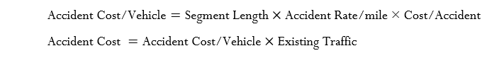
If the capacity of a facility is enhanced (i.e., an increase in supply), the new equilibrium for a given demand curve results in a higher number of trips and a lower user cost per trip, as can be seen in the figure below (equilibrium between supply and demand shifts from point A to point B in the graph).
To determine the user benefits (consumer surplus) for induced traffic, the "rule of half" is applied. This means that the benefits per trip derived from the use of the enhanced facility by induced traffic is half of the additional benefits accruing to existing traffic as a result of the facility enhancement. The logic behind the "rule of half" comes from the shape of the gray area under the demand curve (area ABC) that is created by the facility enhancement, which is a triangle if the demand curve is (approximately) a straight line.
Figure 31: Effect of Induced Demand on User Cost Per Trip and Volumes of Trips
Text description of Figure 31.
Effect of induced demand on user cost per trip and volumes of trips
This figure shows an economic chart demonstrating the impact on user costs per trip and volume of trips from an increase in road capacity. The X axis is "volume of trips" and the Y axis is "user cost per trip." A straight downward sloping diagonal line shows the demand curve. Two upward sloping lines show supply curves. The higher curve is the "No Build" supply curve. The lower curve is the "Build" supply curve. The figure shows the No Build traffic volume and user cost at the intersection of the demand curve and the higher "No Build" supply curve as well as the Build traffic volume and user cost at the intersection of the demand curve and the lower "Build" supply curve. The diagram demonstrates that if the project is built the user cost decreases and the volume of trips increases and that the consumer surplus equals the area below the downward sloping demand curve.
The concept of induced traffic is important to determine user benefits and costs for new and diverted users (i.e., private benefits and costs). These private benefits and costs include:
For costs and benefits that are mainly societal such as emissions, there will be no distinction between induced traffic and existing traffic. In other words, the societal costs of emissions are assumed to be equal for both existing and new traffic.
The users of P3-VALUE 2.2 will be required to provide traffic projections for both the No Build and Build alternatives. Typically, these projections will be generated using a travel demand model. The difference between the No Build and Build traffic projections is induced traffic. These induced traffic projections are then used in the model to calculate the costs and benefits to society of induced traffic.
The total number of trips on a road is determined by traffic demand and supply of roadway capacity. The demand curve shows the relation between the number of trips and user costs per trip. These user costs include tolls, as the user will consider the cost of tolls when deciding whether or not to make a trip. The user cost also includes travel time costs, vehicle operating costs and accident costs. However, users may not consider the costs of emissions in their decision making process. In other words, private costs (including tolls but excluding emissions) ultimately determine the number of trips taken on a road.
For existing traffic, the introduction of tolls or change in toll levels between the No Build and Build alternatives does not modify the calculation of societal benefits. To determine the societal benefits of a facility expansion for existing traffic, the social costs of travel (i.e., excluding tolls which are transfers) for each existing user before and after the expansion are evaluated. The difference in travel costs multiplied by the number of existing users is the net benefit to society of the facility enhancement.
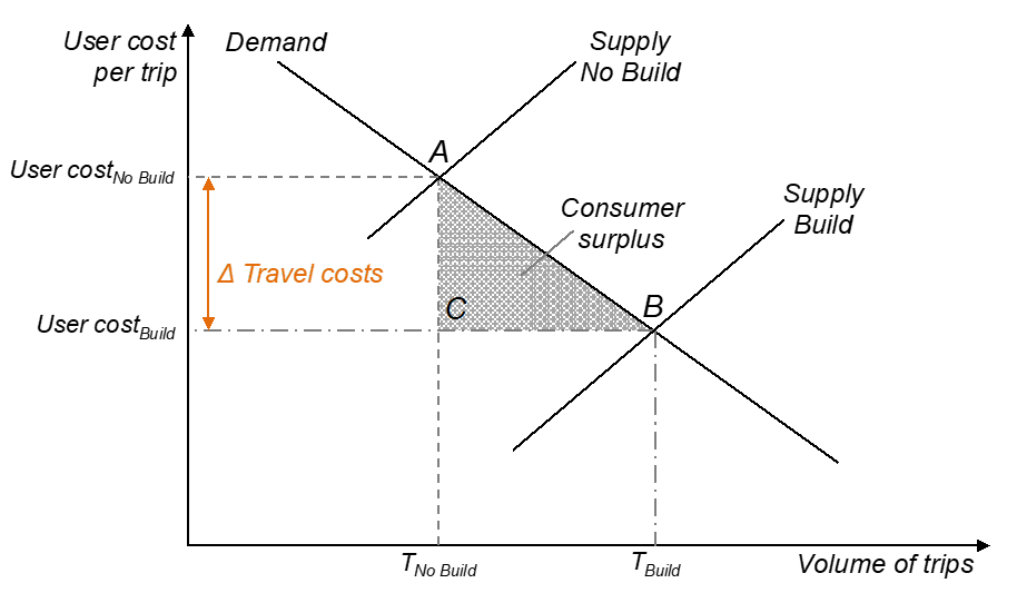
For induced traffic, the rule of half can be used to calculate the societal costs and benefits if both the No Build and Build alternatives are not tolled. However, if the road is tolled in the Build or even in the No Build alternative, the rule of half alone can no longer be applied as the shape under the demand curve that represents the net benefits to society now has both a triangular consumer surplus and a rectangular producer surplus, as can be seen in the figure below. The producer surplus is equal to the toll level under the Build alternative multiplied with the induced traffic (CBDE in the figure below). The consumer surplus calculation (ABC in Figure 32 below) includes the consideration of tolls borne by users under both the Build and the No Build cases.
Figure 32: Effect of Toll on Consumer Surplus and Producer Surplus
Text description of Figure 32.
Effect of toll on consumer surplus and producer surplus
This figure shows an economic chart demonstrating the differences in consumer and producer surplus under the Build and No Build cases if the facility is tolled. The X axis is "volume of trips" and the Y axis is "user cost per trip." A straight downward sloping diagonal line shows the demand curve. Two upward sloping lines show supply curves. The higher curve is the "No Build" supply curve. The lower curve is the "Build" supply curve, which results in a lower user cost per trip and a higher volume of trips. Producer surpluses and consumer surpluses are labeled. They show that if the road is tolled in the Build case, the shape under the demand curve that represents the net benefits to society has a triangular consumer surplus and a rectangular producer surplus. The producer surplus is equal to the toll level under the Build alternative multiplied with the induced traffic. The triangular consumer surplus area is calculated considering tolls borne by users under both the Build and the No Build cases as well as the difference in travel costs and the increase in volume of trips.
P3-VALUE 2.2 calculates the consumer surplus (net benefits to consumers) and the producer surplus (additional benefits to society due to the irrelevance of tolls/transfers from an economic perspective) for induced traffic separately. In P3-VALUE 2.2, consumer and producer surplus are calculated using the following formulae:
![Consumer surplus = 1/2 x (â–³_(user travel costs )+[( toll )] / No Build -[(toll)] / Build) x induced traffic
Producer surplus = [(toll)] / Build x induced traffic](/ipd/images/p3/toolkit/p3_value_2_2/2_6_formula_14.png)
11 P3-VALUE 2.0 traffic calculations distinguish between: 1) GPL vs. ML/TL traffic, 2) peak vs. off peak traffic, 3) weekday vs. weekend traffic, 4) 2 axles vs. 4+ axles traffic, 5) No Build vs. Build traffic. The model uses user inputs (percentage of daily traffic) to compute peak, off-peak, and weekend traffic. In addition, it uses 2 and 4+ axle vehicle percentages for each period (peak, off-peak and weekend) to compute traffic for each vehicle type and period.
12 Assuming a level of service (LOS) E capacity of 2,000 vehicles per lane per hour and a LOS C capacity of 1,500 vehicles per lane per hour.
13 Texas Transportation Institute's (TTI's) Urban Mobility Report, https://mobility.tamu.edu/umr/, as documented in FHWA's TRUCE 3.0 model
14 FHWA's BCA.Net Reference Manual, November 2006
15 Abbreviated Injury Scale
16 Appendix A, "Induced Traffic and Induced Demand" (Lee, et al., 2002) in the HERS-ST v2.0 Technical Report