Appendix C: Transit Investment Analysis Methodology

The Transit Economic Requirements Model (TERM), an analytical tool developed by the Federal Transit Administration (FTA), forecasts transit capital investment needs over a 20-year period. Using a broad array of transit-related data and research, including data on transit capital assets, current service levels and performance, projections of future travel demand, and a set of transit asset-specific condition decay relationships, the model generates the forecasts that appear in the C&P Report.

This appendix provides a brief technical overview of TERM and describes the various methodologies used to generate the estimates for the current (23rd) edition of the C&P Report.

TERM forecasts the level of annual capital expenditures required to attain specific physical condition and performance targets within a 20-year period. These annual expenditure estimates cover the following types of investment needs: (1) asset preservation (rehabilitation and replacement); and (2) asset expansion to support projected ridership growth.

The capital needs forecasted by TERM rely on a broad range of input data and user-defined parameters. Gathered from local transit agencies and the National Transit Database (NTD), the input data are the foundation of the model’s investment needs analysis, and include information on the quantity and value of the Nation’s transit capital stock. The input data in TERM are used to draw an overall picture of the Nation’s transit landscape; the most salient data tables that form the backbone of the TERM database are described below.

The asset inventory data table documents the asset holdings of the Nation’s transit operators. Specifically, these records contain information on each asset’s type, transit mode, age, and expected replacement cost. As the FTA does not directly measure the condition of transit assets, asset condition data are not maintained in this table. Instead, TERM uses asset decay relationships to estimate current and future physical condition as required for each model run. These condition forecasts are then used to determine when each type of asset identified in the asset inventory table is due for either rehabilitation or replacement. The decay relationships are statistical equations that relate asset condition to asset age, maintenance, and utilization. The decay relations and how TERM estimates asset conditions are further explained later in this appendix.

The asset inventory data are derived from a variety of sources, including the NTD, responses by local transit agencies to FTA data requests, and special FTA studies. The asset inventory data table is the primary data source for the information used in TERM’s forecast of preservation needs.

This data table stores demographic information on 486 urbanized areas as well as for 10 regional groupings of rural operators. Fundamental data, such as current and anticipated population, in addition to more transportation-oriented information, such as current levels of vehicle miles traveled (VMT) and transit passenger miles, are used by TERM to predict future transit asset expansion needs.

The agency-mode statistics table contains operations and maintenance (O&M) data on each of the individual modes operated by 845 urbanized area transit agencies and 1,684 rural operators. Specifically, the agency-mode data on annual ridership, passenger miles, operating and maintenance costs, mode speed, and average fare data are used by TERM to help assess current transit performance, future expansion needs, and the expected benefits from future capital investments in each agency-mode (both for preservation and expansion). All the data in this portion of the TERM database come from the most recently published NTD reporting year. Where reported separately, directly operated and contracted services are both merged into a single agency-mode within this table.

The asset type data table identifies approximately 500 different asset types utilized by the Nation’s public transit systems in support of transit service delivery (either directly or indirectly). Each record in this table documents each asset’s type, unit replacement costs, and the expected timing and cost of all life-cycle rehabilitation events. Some of the asset decay relationships used to estimate asset conditions are also included in this data table. The decay relationships—statistically estimated equations relating asset condition to asset age, maintenance, and utilization—are discussed more in the next section of this appendix.

The benefit-cost parameters data table contains values used to evaluate the merit of different types of transit investments forecasted by TERM. Measures in the data table include transit rider values (e.g., value of time and links per trip), auto costs per VMT (e.g., congestion delay, emissions costs, and roadway wear), and auto user costs (e.g., automobile depreciation, insurance, fuel, maintenance, and daily parking costs).

The mode types data table provides generic data on all of the mode types used to support U.S. transit operations—including their average speed, average headway, and average fare—and estimates of transit riders’ responsiveness to changes in fare levels. Similar data are included for nontransit modes, such as private automobile and taxi costs. The data in this table are used to support TERM’s benefit-cost analysis.

The input tables described above form the foundation of TERM, but are not the sole source of information used when modeling investment forecasts. In combination with the input data, which are static—meaning that the model user does not manipulate them from one model run to the next—TERM contains user-defined parameters to facilitate its capital expenditure forecasts.

As part of its investment needs analysis, TERM predicts the current and expected future physical condition of U.S. transit assets over a 20-year period. These condition forecasts are then used to determine when each of the individual assets identified in the asset inventory table are due for either rehabilitation or replacement. The investment policy parameters data table allows the user to set the physical condition ratings at which rehabilitation or replacement investments are scheduled to take place (though the actual timing of rehabilitation and replacement events may be deferred if the analysis is budget-constrained). Unique replacement condition thresholds may be chosen for the following asset categories: guideway elements, facilities, systems, stations, and vehicles. For the current (23rd) edition of the C&P Report, all of TERM’s replacement condition thresholds have been set to trigger asset replacement at condition 2.5. (Under the Sustain 2014 Spending scenario, many of these replacements would be deferred due to insufficient funding capacity.)

In addition to varying the replacement condition, users can vary other key input assumptions intended to better reflect the circumstances under which existing assets are replaced and the varying cost impacts of those circumstances. For example, users can assume that existing assets are replaced under full service, partial service, or a service shutdown. Users can also assume assets are replaced either by agency (force-account) or by contracted labor. Each of these affects the cost of asset replacement for rail assets.

TERM also includes two key financial parameters. First, the model allows the user to establish the rate of inflation used to escalate the cost of asset replacements for TERM’s needs forecasts. Note that this feature is not used for the C&P Report, which reports all needs in current dollars. Second, users can adjust the discount rate used for TERM’s benefit-cost analysis.

The data tables described above allow TERM to estimate different types of capital investments, including rehabilitation and replacement expenditures, expansion investments, and capital projects aimed at performance improvements. These three different investment categories are described below.

TERM’s asset rehabilitation and replacement forecasts are designed to estimate annual investments for the ongoing rehabilitation and replacement of the Nation’s existing transit assets. Specifically, these needs include the normal replacement of assets reaching the end of their useful life, mid-life rehabilitations, and annual “capital expenditures” to cover the cost of smaller capital reinvestment amounts not included as part of asset replacement or rehabilitation activities.

To estimate continuing replacement and rehabilitation investments, TERM estimates the current and expected future physical condition of each transit asset identified in TERM’s asset inventory for each year of the 20-year forecast. These projected condition values are then used to determine when individual assets will require rehabilitation or replacement. TERM also maintains an output record of this condition forecast to assess the impacts of alternate levels of capital reinvestment on asset conditions (both for individual assets and in aggregate). In TERM, the physical conditions of all assets are measured using a numeric scale of 5 through 1; see Exhibit C-1 for a description of the scale.

---

Exhibit C-1: Definitions of Transit Asset Conditions

Rating	Condition	Description
Excellent	4.8–5.0	No visible defects, near new condition.
Good	4.0–4.7	Some slightly defective or deteriorated components.
Adequate	3.0–3.9	Moderately defective or deteriorated components.
Marginal	2.0–2.9	Defective or deteriorated components in need of replacement.
Poor	1.0–1.9	Seriously damaged components in need of immediate repair.

Source: Transit Economic Requirements Model.

TERM currently allows an asset to be rehabilitated up to five times throughout its life cycle before being replaced. During a life-cycle simulation, TERM records the cost and timing of each reinvestment event as a model output and adds it to the tally of national investment needs (provided they pass a benefit-cost test, if applied).

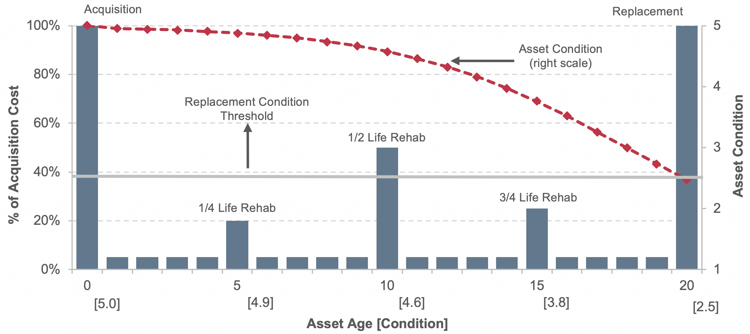
TERM’s process of estimating rehabilitation and replacement needs is represented conceptually for a generic asset in Exhibit C-2. In this theoretical example, asset age is shown on the horizontal axis, the cost of life-cycle capital investments is shown on the left vertical axis (as a percentage of acquisition cost), and asset conditions are shown on the right vertical axis. At the acquisition date, each asset is assigned an initial condition rating of 5, or “excellent,” and the asset’s initial purchase cost is represented by the tall vertical bar at the left of the chart. Over time, the asset’s condition begins to decline in response to age and use, represented by the dotted line, requiring periodic life-cycle improvements including annual capital maintenance and periodic rehabilitation projects. Finally, the asset reaches the end of its useful life, defined in this example as a physical condition rating of 2.5, at which point the asset is retired and replaced.

---

Exhibit C-2: Scale for Determining Asset Condition Over Time, From Acquisition to Replacement

In addition to devoting capital to the preservation of existing assets, most transit agencies invest in expansion assets to support ongoing growth in transit ridership. To simulate these expansion needs, TERM continually invests in new transit fleet capacity as required to maintain at current levels the ratio of peak vehicles to transit passenger miles. The rate of expansion is projected individually for each of the Nation’s 487 urbanized areas (e.g., based on the urbanized area’s specific growth rate projections or historical rates of transit passenger mile growth), while the expansion needs are determined at the individual agency-mode level. TERM will not invest in expansion assets for agency-modes with current ridership per peak vehicle levels that are well below the national average (these agency-modes can become eligible for expansion during a 20-year model run if there is sufficient projected growth in ridership for them to rise above the expansion investment threshold).

In addition to forecasting fleet expansion requirements to support the projected ridership increases, the model also forecasts expansion investments in other assets needed to support that fleet expansion. This includes investment in maintenance facilities and, in the case of rail systems, additional guideway miles including guideway structure, trackwork, stations, train control, and traction power systems. Like other investments forecast by the model, TERM can subject all asset expansion investments to a benefit-cost analysis. Finally, as TERM adds the cost of newly acquired vehicles and supporting infrastructure to its tally of investment needs, it also ensures that the cost of rehabilitating and replacing the new assets is accounted for during the 20-year period of analysis.

TERM’s estimates for capital expansion needs in the Low and High Growth scenarios are driven by the trend rate of growth in passenger miles traveled (PMT), calculated as the compound average annual PMT growth by FTA region, urbanized area (UZA) stratum, and mode over the most recent 15-year period (hence, all bus operators located in the same FTA region in UZAs of the same population stratum are assigned the same growth rate).

Use of the 10 FTA regions captures regional differences in PMT growth, while use of population strata (over 1 million population, 1 million to 500,000, 500,000 to 250,000 and under 250,000) captures differences in urban area size.

The approach recognizes differences in PMT growth trends by mode. Over the past decade, the rate of PMT growth has differed significantly across transit modes, being highest for heavy rail, vanpool, and demand-response, and low to flat for motor bus. These differences are recognized in the Low and High Growth scenario expansion needs projections.

TERM asset decay curves were developed expressly for use within TERM and are comparable to asset decay curves used in other modes of transportation and bridge and pavement deterioration models. While the collection of asset condition data is not uncommon within the transit industry, TERM asset decay curves are believed to be the only such curves developed at a national level for transit assets. Most of the TERM key decay curves were developed using data collected by FTA at multiple U.S. transit properties specifically for this purpose.

TERM decay curves serve two primary functions: (1) to estimate the physical conditions of groups of transit assets and (2) to determine the timing of rehabilitation and replacement reinvestment.

One use of the decay curves is to estimate the current and future physical conditions of groups of transit assets. The groups can reflect all of the national transit assets or specific subsets, such as all assets for a specific mode. For example, Exhibit C-3 presents a TERM analysis of the distribution of transit asset conditions at the national level as of 2014.

This exhibit shows the proportion and replacement value of assets in each condition category (excellent, good, etc.) segmented by asset category. TERM produced this analysis by first using the decay curves to estimate the condition of individual assets identified in the inventory of the national transit assets, and then grouping these individual asset condition results by asset type.

TERM also uses the decay curves to predict expected future asset conditions under differing capital reinvestment funding scenarios. An example of this type of analysis is presented in Exhibits C-4 and C-5, which present TERM forecasts of the future condition of the national transit assets assuming the national level of reinvestment remains unchanged. Exhibit C-4 shows the future condition values estimated for each of the individual assets identified in the asset inventory (weighted by replacement value) to generate annual point estimates of average future conditions at the national level by asset category. Exhibit C-5 presents a forecast of the proportion of assets in either marginal or poor condition, assuming limited reinvestment funding for a subset of the national transit assets.

---

Exhibit C-3: Distribution of Asset Physical Condition by Asset Type for All Modes, 2014

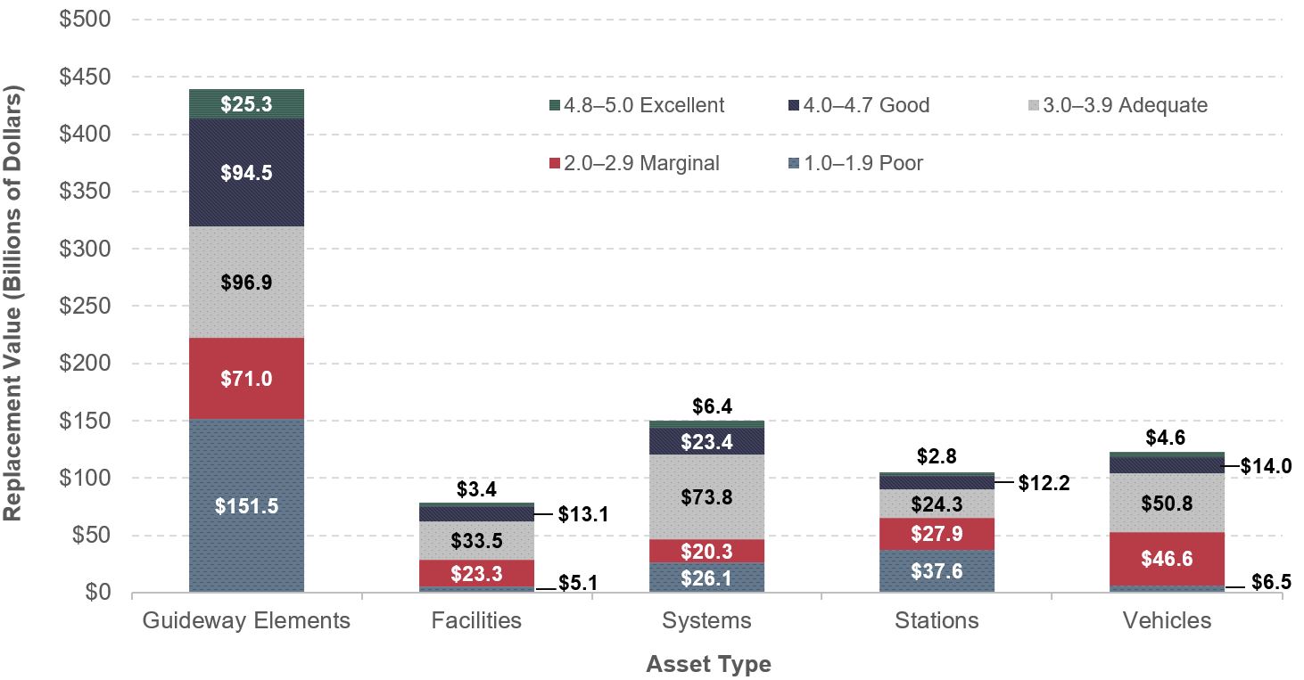
Source: Transit Economics Requirements Model.

---

Exhibit C-4: Weighted Average by Asset Category, 2014–2033

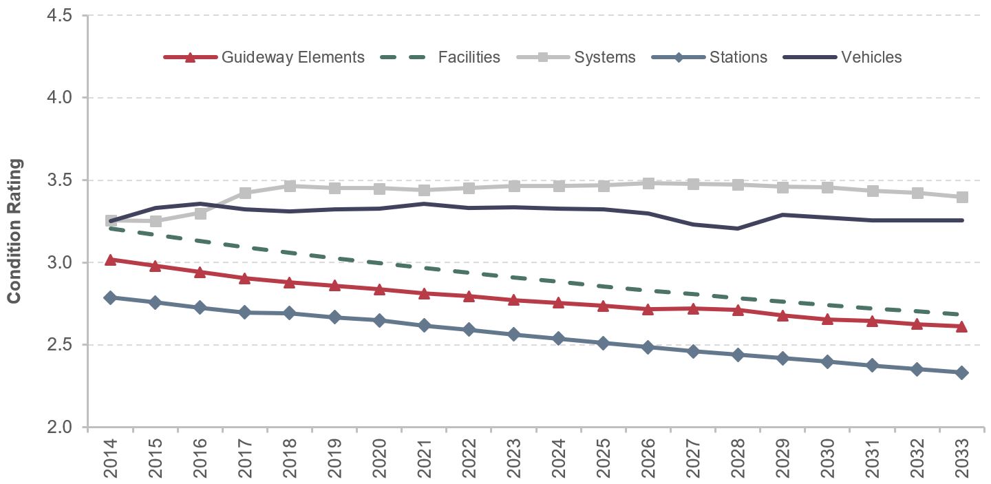
Source: TERM, Sustain 2014 Spending.

---

Exhibit C-5: Assets in Marginal or Poor Condition, 2014–2033

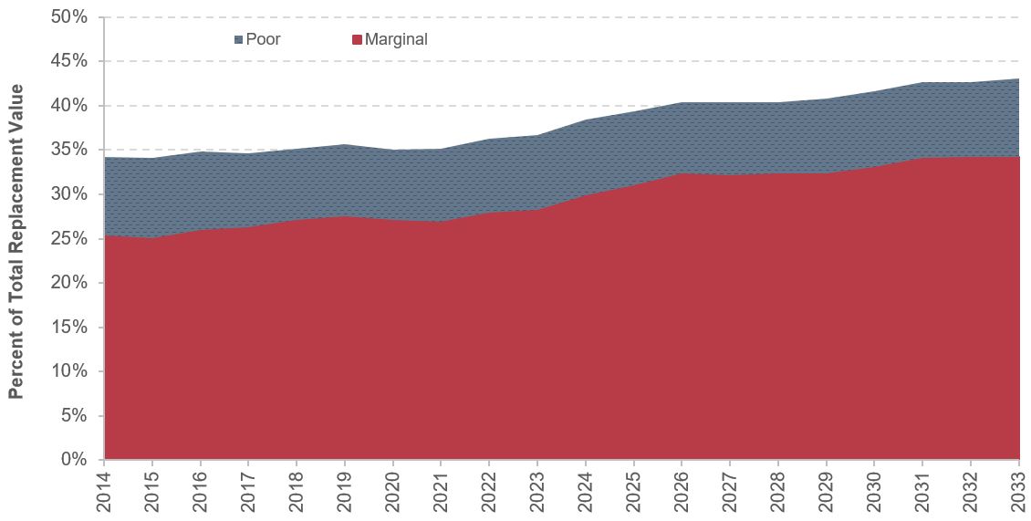
Source: TERM, Sustain 2014 Spending (Excludes Unreplaceable Assets).

Another key use of the TERM asset decay curves is to determine when the individual assets identified in the asset inventory will require either rehabilitation or replacement, with the ultimate objective of estimating replacement needs and the size of the state of good repair (SGR) backlog. Over the 20-year period of analysis covered by a typical TERM simulation, the model uses the decay curves to continually monitor the declining condition of individual transit assets as they age. As an asset’s estimated condition value falls below predefined threshold levels (known as “rehabilitation condition threshold” and “replacement condition threshold”), TERM will seek to rehabilitate or replace that asset accordingly. If sufficient funding is available to address the need, TERM will record this investment action as a need for the specific period in which it occurs. If insufficient funding remains to address a need, that need will be added to the SGR backlog. These rehabilitation and replacement condition thresholds are controlled by asset type and can be changed by the user. Some asset types, such as maintenance facilities, undergo periodic rehabilitation while others, such as radios, do not.

Asset decay curves are statistically estimated mathematical formulas that rate the physical condition of transit assets on a numeric scale of 5 (excellent) to 1 (poor).

The majority of TERM decay curves are based on empirical condition data obtained from a broad sample of U.S. transit operators; hence, they are considered to be representative of transit asset decay processes at the national level. An example decay curve showing bus asset condition as a function of age and preventive maintenance based on observations of roughly 900 buses at 43 different transit operators is presented in Exhibit C-6.

---

Exhibit C-6: TERM Asset Decay Curve for 40-Foot Buses

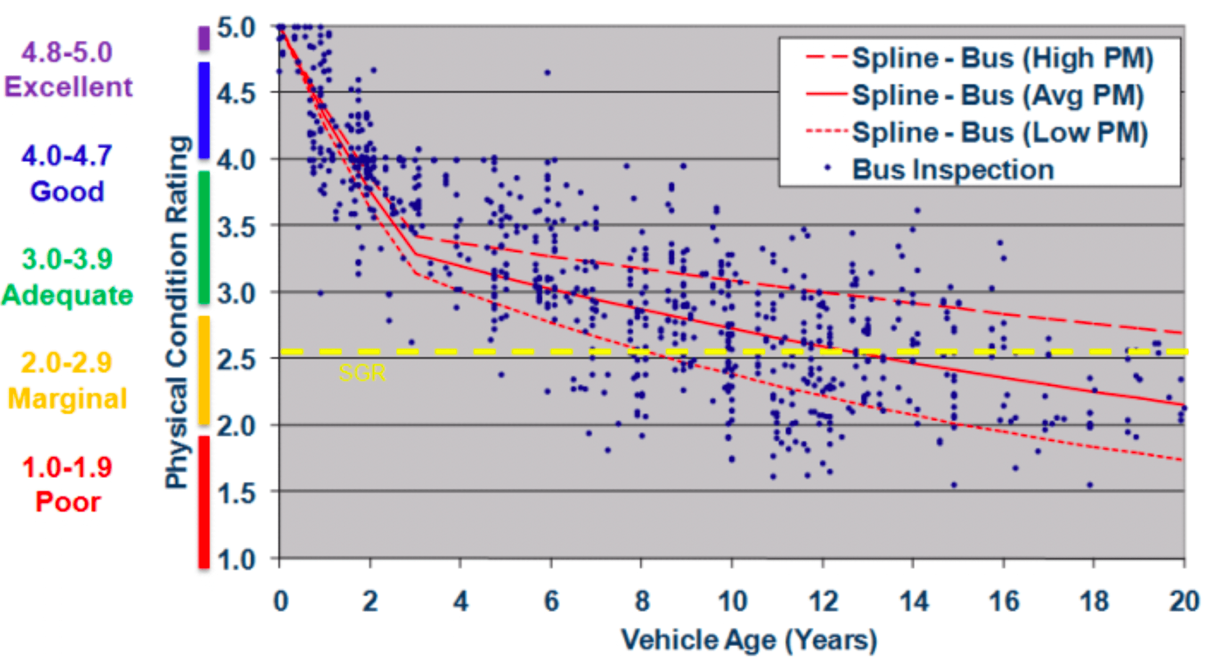
Source: FTA; empirical condition data obtained from a broad sample of U.S. transit operators.

TERM uses a benefit-cost (B/C) module to assess which of a scenario’s capital investments are cost-effective and which are not. The purpose of this module is to identify and filter investments that are not cost-effective from the tally of national transit capital needs. Specifically, TERM can filter all investments where the present value of investment costs exceeds investment benefits (BCR<1).

The TERM B/C module is a business case assessment of each agency-mode (e.g., “Metroville Bus” or “Urban City Rail”) identified in the NTD. Rather than assessing the BCR for each individual investment need for each agency-mode (e.g., replacing a worn segment of track for Urban City Rail), the module compares the stream of future benefits arising from continued future operation for an entire agency-mode against all capital (rehab-replace and expansion) and operating costs required to keep that agency-mode in service. If the discounted stream of benefits exceeds the costs, then TERM includes that agency-mode’s capital needs in the tally of national investment needs. If the net present value of that agency-mode investment is less than zero (BCR<1), then TERM scales back these agency-mode needs until the benefits are equal to costs as discussed below.

In effect, the TERM B/C module conducts a systemwide business case analysis to determine if the value generated by an existing agency-mode is sufficient to warrant the projected cost to operate, maintain, and potentially expand that agency-mode. If an agency-mode does not pass this systemwide business case assessment, then TERM will not include some or all of that agency-mode’s identified reinvestment needs in the tally of national investment needs. The benefits assessed in this analysis include user, agency, and social benefits of continued agency operations.

TERM considers the cost-benefit of the entire agency rail investment versus simply considering the replacement of a single rail car. Costs and benefits are grouped into an aggregated investment evaluation and not evaluated at the level of individual asset investment actions (e.g., replacement of a segment of track) for two primary reasons: (1) lack of empirical benefits data, and (2) transit asset interrelationships.

Lack of Empirical Benefits Data: The marginal benefits of transit asset reinvestment are very poorly understood for some asset types (e.g., vehicles) and nonexistent for others. Consider this example: replacement of an aging motor bus will generate benefits in the form of reduced maintenance costs, improved reliability (fewer in-service failures and delays) and improved rider comfort, and potentially increased ridership in response to these benefits. The magnitude of each of these benefits will be dependent on the age of the vehicle retired (with benefits increasing with increasing age of the vehicle being replaced). But what is the dollar value of these benefits? Despite the fact that transit buses are the most numerous of all transit assets and a primary component of most transit operations, the relationship between bus vehicle age and O&M cost, reliability, and the value of rider comfort is poorly understood (there are no industry standard metrics tying bus age to reliability and related agency costs). The availability of reinvestment benefits for other transit asset types is even more limited (perhaps with the exception of rail cars, where the understanding is comparable to that of bus vehicles).

Transit Asset Interrelationships: The absence of empirical data on the benefits of transit asset replacement is further compounded by both the large number of transit assets that must work together to support transit service and the high level of interrelatedness between many of these assets. Consider the example of a (1) rail car operating on (2) trackwork equipped with (3) train control circuits and (4) power supply (running through the track), all supported by (4) a central train control system and located on (5) a foundation such as elevated structure, subway, retained embankment, etc. This situation represents a system that is dependent on the ongoing operation of multiple assets, each with differing costs, life cycles, and reinvestment needs and yet totally interdependent on one another. Now consider the benefits of replacing a segment of track that has failed. The cost of replacement (thousands of dollars) is insignificant compared with the benefits derived from all the riders that depend on that rail line for transit service of maintaining system operations. The fallacy in making this comparison is that the rail line benefits are dependent on ongoing reinvestment in all components of that rail line (track, structures, control systems, electrification, vehicles, and stations) and not just from reinvestment in specific components.

TERM’s B/C module is designed to assess the benefits of incremental levels of reinvestment in each agency-mode in a three-step approach:

• Step 1: TERM begins its benefit-cost assessment by considering the benefits derived from all of TERM’s proposed capital investment actions for a given agency-mode—including all identified rehabilitation, replacement, and expansion investments. If the total stream of benefits from these investments exceeds the costs, then all assets for this agency-mode are assigned the same (passing) benefit-cost ratio. If not, then the B/C module proceeds to Step 2.
• Step 2: Having “failed” the Step 1 B/C test, TERM repeats this B/C evaluation, but this time excludes all expansion investments. In effect, this test suggests that this agency-mode does not generate sufficient benefits to warrant expansion but may generate enough benefits to warrant full reinvestment. If the agency-mode passes this test, then all reinvestment actions are assigned the same, passing benefit-cost ratio. Similarly, all expansion investments are assigned the same failing benefit-cost ratio (as calculated in Step 1). If the agency-mode fails the Step 2 B/C test, the B/C module proceeds to Step 3.
• Step 3: The Step 3 B/C test provides a more realistic assessment of agency-mode benefits. Under this test, it is assumed that agency-mode benefits exceed costs for at least some portion of that agency-mode’s operations; hence, this portion of services is worth maintaining.

TERM’s B/C module segments investment benefits into three groups of beneficiaries:

• transit riders (user benefits),
• transit operators, and
• society.

Rider Benefits: By far the largest individual source of investment benefits (roughly 86 percent of total benefits) accrue to transit riders. Moreover, as assessed by TERM, these benefits are measured as the difference in total trip cost between a trip made via the agency-mode under analysis versus the agency-mode user’s next best alternative. The total trip cost includes both out-of-pocket costs (e.g., transit fare, station parking fee) and value of time costs (including access time, wait time, and in-vehicle travel time).

Transit Agency Benefits: In general, the primary benefit to transit agencies of reinvestment in existing assets comes from the reduction in asset O&M costs. In addition to fewer asset repair requirements, this benefit includes reductions of in-service failures (technically also a benefit to riders) and the associated in-service failures response costs (e.g., bus vehicle towing and substitution, bus for rail vehicle failures).

At present, none of these agency benefits is considered by TERM’s B/C model. As noted above, there are little to no data to measure these cost savings. That said, there are some data on which to evaluate these benefits, mostly related to fleet reinvestment and not available at the time the B/C module was developed. FTA could move to incorporate some of these benefits in future versions of TERM.

Societal Benefits: TERM assumes that investment in transit provides benefits to society by maintaining or expanding an alternative to travel by car. More specifically, reductions in VMT made possible by the existence or expansion of transit assets are assumed to generate benefits to society. Some of these benefits may include reductions in highway congestion, air and noise pollution, energy consumption, and automobile accidents. TERM’s B/C module does not consider any societal benefits beyond those related to reducing VMT (hence, benefits such as improved access to work are not considered).

The analysis of the SGR backlog—a measure of the total value of deferred transit capital investment at the national level—is motivated by two main concerns:

1. the high backlog value relative to existing funding capacity, and
2. projections suggesting the backlog will continue to grow if funding levels are maintained for the foreseeable future.

The text that follows provides a brief overview of the SGR backlog measure, including the measure’s definition and the data and methods used to estimate its size. It also describes limiting factors that affect the accuracy and comparability of the backlog size published in different editions of the C&P Report.

The SGR backlog provides an estimate of the total level of capital reinvestment required to eliminate all outstanding reinvestment needs and thus bring the nation’s transit assets to a full state of good repair. This should in principle include investment to replace all assets that currently exceed their service life and to repair all assets with outstanding rehabilitation needs.

However, estimates for this and previous editions of the C&P Report are subjected to four main limitations:

1. The estimate of current backlog size is focused solely on deferred replacement needs, and thus does not include an assessment of deferred rehabilitation needs. As such, the current backlog estimate is necessarily a lower-bound estimate of the actual SGR backlog.
2. The asset inventory data provide only information on asset age or overall condition. These data are sufficient to estimate replacement needs, but not rehabilitation needs.
3. TERM provides estimates of future rehabilitation needs based on the typical life-cycle reinvestment needs of transit assets. However, as the underlying asset inventory data sources are not designed to report the extent to which an asset’s expected rehabilitation actions have been performed, TERM has no basis on which to estimate the current level of deferred rehabilitation needs.
4. TERM’s backlog estimates are limited primarily to those assets owned by FTA grantees. Hence, the estimates tend to exclude the reinvestment needs of some assets that are used for transit service but not owned by a grantee. For example, it excludes some assets that are leased by the grantee, provided for service by a municipality, or provided through track access agreements. This resulting level of backlog underestimation is thought to be minor.

Backlog is estimated from two different sources:

1. NTD data on vehicle assets, including vehicle types, quantities, and ages of all rail cars, buses, vans, and other revenue vehicles used by grantees to provide transit service.
2. Data requests to a sample of the nation’s largest (primarily rail) operators and special studies for all other asset categories.

Data requests were obtained at a time when data collection, recording, and classification were not standardized. Therefore, data provided to FTA vary significantly in level of detail, content, and quality from one operator to the next. Moreover, in response to the transit industry’s movement toward improved asset management practices, the level of reported inventory detail, format, and data quality obtained through direct grantee requests has been and continues to undergo significant change. The nature and magnitude of these ongoing changes in local agency inventory quality and level of detail has similarly resulted in significant changes to the national inventory dataset on which TERM relies. Consequently, these changes result in inventory datasets and backlog estimates that are not strictly comparable from one C&P Report to the next.

In addition to data standardization and quality, the accuracy of the SGR backlog estimate and investment needs is affected by TERM’s methodology and assumptions. Specifically, the shape of the decay curves used to model asset condition and the condition threshold selected for asset replacement (currently condition level 2.5) have a significant impact on the size of the backlog estimate, as shown in Exhibit C-7.

---

Exhibit C-7: Backlog Estimate vs Replacement Threshold

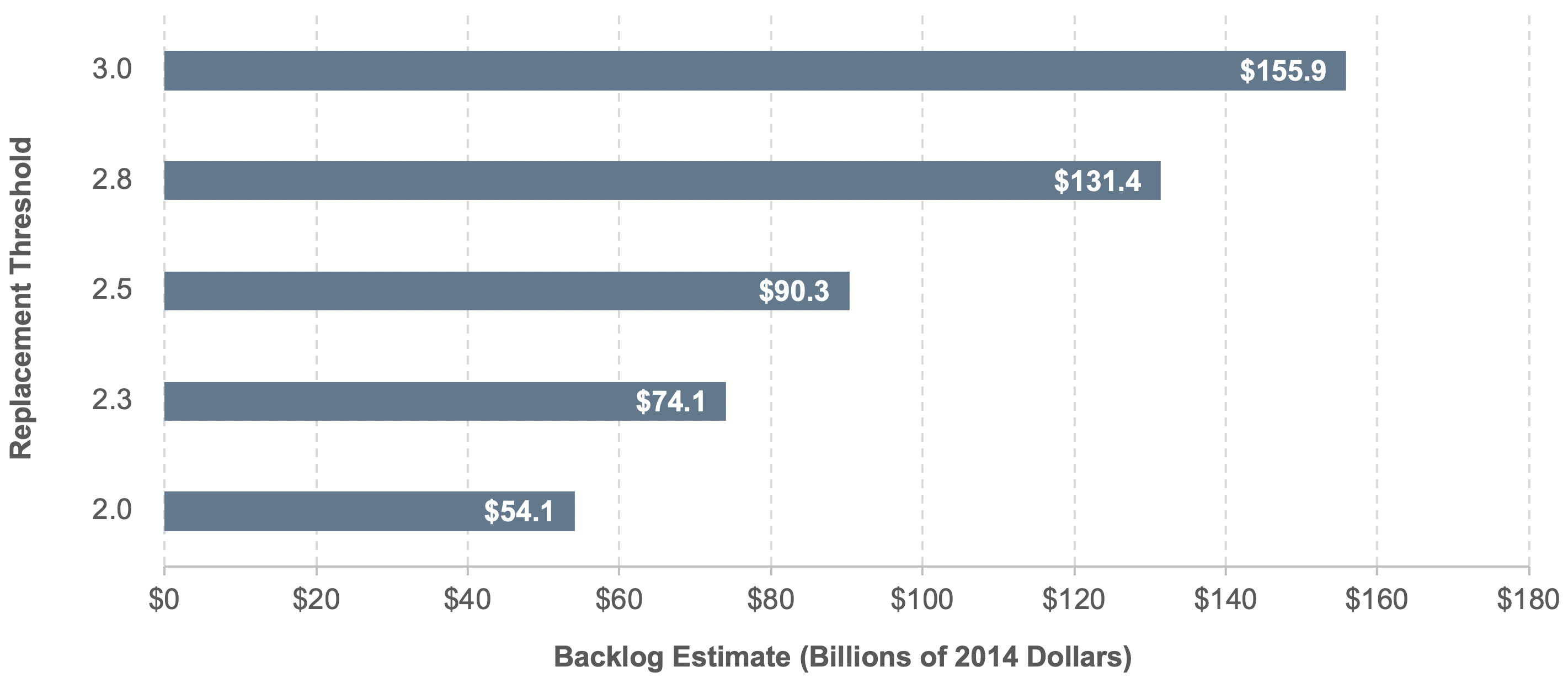
Source: Transit Economic Requirements Model.

Many of issues addressed in this appendix will be significantly mitigated or eliminated following the implementation of the expanded and standardized Asset Inventory Module (AIM), implemented over 2018–2020. Under the new reporting requirements, all grantees will report the age and quantities of their asset holdings in AIM, after which inventory data requests will no longer be required.